Monopoly, Inequality and Redistribution via the Public Provision of Private Goods

Working Paper Series

Monopoly, Inequality and Redistribution via the

Public Provision of Private Goods

Margarita Katsimi

Thomas Moutos

ECINEQ 2006-29

March

2006

www.ecineq.org

Monopoly, Inequality and Redistribution via the Public

Provision of Private Goods

*

Margarita Katsimi and Thomas Moutos

†

AUEB and CESifo

Abstract

The relationship between inequality and redistribution is usually studied under the assumption that the government collects different amounts of taxes from each citizen (voter) but gives back the same amount (in cash or in kind) to everyone. In this paper we consider what happens if the government can redistribute through both sides of its budget (revenue and expenditure). We study the effects of inequality on the size (and structure) of redistributive programs in both perfectly competitive and monopolistic settings. We find that the presence of monopoly results in a higher tax rate than in the competitive case and that in the latter case an increase in inequality can be associated with a fall in the tax rate. We find also that although the median voter may not vote for a positive tax rate in the presence of public sector inefficiency under perfect competition, she may prefer – ceteris paribus – a positive tax rate in the presence of monopoly.

Keywords: Monopoly, Redistribution, Inequality, Public Goods, Median Voter JEL Classification: H23, H42, P16.

1. Introduction

Following the influential contributions of Romer (1975), Meltzer and Richard (1981),

Alesina and Rodrik (1994) and Persson and Tabellini (1994), the conventional wisdom is that higher income inequality among voters leads to increased government redistribution. The intuition behind this result is that the greater is the gap between median and mean income, the higher will be the level of spending preferred by the median income voter and – since political competition drives policy decisions toward the ideal point of the median income voter – the higher will be the equilibrium amount of redistribution. Nevertheless, despite some empirical evidence in support of this hypothesis (see, Meltzer and Richard (1983), Milanovic (2000)), other empirical studies have not found that higher income inequality among voters leads to an increase in the size of redistributive programs (see, for example, Clarke (1995), Perotti (1996) and Rodriguez (1999)). This has led some (e.g., Benabou (1996) and Rodriguez (1999)) to urge the profession to take seriously the need to relax median voter assumptions in order to gain an understanding in variations in redistributive activity across countries and over time.

Political scientists have long argued that unadulterated, fully participatory, median-voter democracy describes no actual political system – rather, the translation of resources into influence occurs in highly institutionalized environments that amplify some voices and mute others. Although we do not want to dispute the validity of this claim, in this paper we show that the median voter-framework can generate a more diverse set of outcomes once we take into account that redistribution is often effected through the public provision of private goods1. Moreover, we demonstrate that if the assumption of perfect competition is relaxed

1 _{Other papers showing that there is not, necessarily, a divergence between theory (based on the median-voter}

framework) and empirical evidence include Lee and Roemer (1999), Benabou (2000), Saint-Paul (2001) and Alesina, Glaeser and Sacerdote (2001).

(i.e., monopoly), the median-voter's preferred policy will involve -ceteris paribus- a higher tax rate than in the perfectly competitive case. We also find that the median voter will be willing to support redistributive policies under monopoly even when, due to public sector inefficiency, under perfectly competitive conditions the median voter would prefer no public provision.

Our finding that the relationship between inequality and redistribution is not positive once we assume that redistribution is effected through the public provision of private goods is not novel. Indeed, Grossman (2003) has shown that higher inequality of capital endowments may reduce redistribution if the government uses the tax proceeds to finance public provision of a homogeneous good rather than (income) transfers. Both poor and rich households in

Grossman's model have no choice other than consuming the freely-provided public good. In contrast, in the present paper the government uses the tax proceeds to finance the provision of a rival public good which is also provided by the private sector, albeit at different quality levels – a vertically differentiated product (VDP) like health, education, or day care2. Households are assumed to derive utility from the consumption of the VDP (either of the variety freely provided by the government or of one of the varieties offered by the private sector) and of a privately produced homogeneous product. We assume that both goods are rival in consumption. This implies that if a higher proportion of households decide to

2 _{Our modeling follows Besley and Coate (1991) (see, also, Munro (1991), Boadway and Marchand (1995),}

Blomquist and Christiansen (1995, 1999), Thum and Thum (2002)) who used the idea that people with different incomes can value publicly provided goods differently, in order to show how public provision can induce self-selection (e.g. only the poor choose to consume the relatively low quality of the good provided by the

government - with the rich prefering to avail themselves of higher quality varieties which are privately supplied) and achieve redistribution with lower efficiency costs than if cash transfers were used.

5 _{Although the nature of these results is not affected by using other imperfectly competitive settings (e.g.,}

“consume” the publicly provided variety, the quality provided by the public sector must decline. Thus, if in response to higher income inequality the median voter would otherwise have chosen to vote for a higher tax rate, she must now also take into account that a rise in the tax rate may induce a larger number of the more wealthy households to consume the publicly provided variety (since their after-tax income declines). Consequently, the rise in the tax rate may leave the median voter with lower after-tax income without a corresponding rise in the quality of the publicly-provided variety. As a result, the median voter may not prefer a rise in the tax rate as inequality increases. In fact, our results indicate that if the private VDP is produced under perfectly competitive conditions, the median voter equilibrium tax rate will depend negatively on the level of inequality.

To our knowledge, the relationship between inequality and redistribution has been studied only under perfectly competitive settings. In this respect, the more interesting results of our analysis relate to the presence of imperfect competition in the production of the VDP. We find that, first, the equilibrium tax rate will be higher under monopoly than in the perfectly competitive case, second, that the relationship between the equilibrium tax rate and

inequality becomes hump-shaped, and third, that the presence of monopoly can induce the median voter to prefer a positive tax rate, even in cases where the inefficiency of the public sector relative to the private sector is so large that the median voter would not vote for a positive tax rate under perfectly competitive conditions (i.e., the presence of monopoly can result in the public provision of private goods even in case of “government failure”)5_{. The}

explanation for the above results rests on the fact that the median voter realizes that the presence of – even an inefficient - public sector, in effect, allows her to avoid paying a price above marginal cost, and that the incomes of those consuming the privately (monopoly) supplied variety will be further at the upper-tail of the income distribution than in the

perfectly competitive case. Consequently, the median voter expects that a rise in the tax rate will increase the number of households deciding to consume the publicly provided variety by a smaller number in the monopoly case –thus making the “congestion costs” of a higher tax rate smaller.

Our finding that the relationship between the equilibrium tax rate and inequality becomes hump-shaped is driven by the positive impact of inequality on the mark-up of monopoly prices over cost. At a high level of inequality, the mark-up of monopoly prices is such that only very high-income individuals will consume the privately-supplied variety. In that case, an increase in inequality will induce the median voter to choose a higher tax rate since the thinning tail of the income distribution ensures that the ‘redistribution’ effect of a tax rise is stronger than the implied ‘congestion’ effect. On the other hand, when inequality is low the monopoly prices are close to cost so that the relationship between inequality and taxes is similar to the perfectly competitive case.

The rest of the paper is organized as follows: The basic model is described in section 2. The median voter equilibrium size of government is derived in section 3. Section 4 relaxes the assumption of perfect competition and introduces the case of monopoly. Section 5 concludes.

2. The Model

Consider a closed economy which produces and consumes two goods (X and Y) with the use of labour. We assume that perfect competition prevails in all markets and that all households (citizens-cum-voters) are endowed with one unit of labor, which they offer inelastically. There are, however, differences in skill between households, which are reflected in differences in the endowment of each household’s effective labor supply. This is in turn

reflected in differences in income across households. We assume that firms pay the same wage rate per effective unit of labor –thus the distribution of talent across firms does not affect unit production costs. We will assume that the politico-economic equilibrium is determined according to the Downsian model of electoral competition.

a. Firms

Good X is a homogeneous good produced only by private sector firms under linear technology,

X =L, (1) whereLstands for the effective units of labour used. Using labour as the numeraire, we get

that the price of goodX , p_X, is unity.

Good Yis a vertically differentiated good (VDP) which is produced at various quality levels

in both the private and the public sector. We wish to capture the fact that, for many

government-provided goods (or services), some citizens choose not to “consume” them (even though they are eligible for doing so and there is no price-tag attached to them), preferring instead to purchase them from the private sector. Typical examples of such publicly provided goods are health care, child care, old-age care and education. One reason for this

phenomenon is that these goods are vertically differentiated according to quality (thus displaying large income elasticity) and there is a large degree of lumpiness associated with their consumption. For example, it is nearly impossible for a student to attend at the same time a public and a private educational institution (or to attend both part-time thus achieving a full-time status), or for a patient to have part of a heart operation at a public hospital and the rest of the operation at a private one. Moreover, in many cases it confers no extra utility (or it is detrimental) to supplement publicly provided goods with privately provided ones (i.e., first

having an operation at a public hospital and afterwards supplementing it with another operation at a private hospital). Wealthy households will often elect to pay in order to avail themselves of the highest quality of these services – rather than be satisfied with the

(sometimes) mediocre quality offered by the public sector.

We assume that quality is measured by an index Q>0, and that there is complete information regarding the quality index. We further assume that for private sector firms average costs depend on quality and that, for any given quality level, the average cost is independent of the number of units produced. These assumptions are captured by the following production function,

/

Q

Y =L βQ β ≤1. (2) In equation (2), Y_Q denotes the number of units of quality Q produced. This particular

specification implies that as quality increases more (effective) units of labour are required to produce each unit of the Ygood. It also implies that the (average cost) and price at which

each variety of the good will be offered is ( ) ( )

AC Q =P Q =βQ. (3) For simplicity, and without loss of generality, we assume that the public sector uses a similar technology to produce the good, pays the same wage rate, but for various reasons may be a less efficient producer than private sector firms3. We capture this (potential) difference in efficiency between the private and the public sector by assuming that average costs in the public sector are

( )

G

AC Q =Q ,

where the superscript G denotes the public sector.

b. Households

All households are assumed to have identical preferences. Following Rosen (1974) and Flam and Helpman (1987), we assume that the homogeneous good is divisible, whereas the quality-differentiated product is indivisible and households can consume only one unit of it. For simplicity - and with some loss of generality - we write the utility function as4

i i i

U = Q X

where X_i and Q_istand for the quantity of the homogeneous good and the quality of good

Y(the VDP) consumed by household i.

Let e_i stand for household’s i endowment of effective number of labour units. Since the

wage rate per effective units of labour is unity, e_ialso stands for household income. We

assume that there is a continuum of households,i∈

[ ]

0,1 , with Pareto distributed incomes. The Pareto distribution is defined over the interval e b≥ , and its CDF is

_{F e}( ) 1 ( / ) ,_{= − b e} a _a>1_{. (4)}

Parameter b stands for the lowest income, and parameter adetermines the shape of the distribution (higher values of aimply greater equality). The Pareto distribution, in addition to being easy to work with, is a good approximation of actual income distributions. Empirical estimates of the value of a range between 1.7 and 3.0 (see, Creedy (1977)). The mean of the Pareto distribution is equal to

µ

=ab a/( −1), (5) and the income of the median voter (household) is

Since good Y is also offered by the public sector, and households can consume either a privately-provided variety or the (single) variety provided by the government, in effect households face two mutually exclusive budget constraints. The budget constraint of a household deciding to acquire a variety of Y which is offered by the private sector is

(1

e

_i −t)

=

P Q

( )

+

P X

_{X i}

=

β

Q X

_i

+

_i ,

whereas, if the household chooses to consume the publicly (and freely) provided variety the budget constraint is,

e

_i

(1 )

− =

t

X

_i ,

where t stands for the income tax rate. Let _QG_{stand for the quality of good Yprovided by}

the public sector. Then, if the household consumes a privately provided variety, the utility maximizing demands for Q and X are (we assume that for all households income is high

enough to generate positive demand for both goods), (1 ) / 2 i i Q =e −t β (7) (1 ) / 2 i i X =e −t (8) whereas if the household consumes the publicly provided variety, the entire disposable

income of the household (=e_i(1−t)) is spent on X .

The resulting indirect utility of the household in the two cases is then,

(1 ) /

P i i

V =e −t β , if it chooses a privately-offered variety, (9)

(1 )

G G

i i

V = e −t Q , if it consumes the publicly-offered variety. (10) We note that the difference between P

i

V and G i

V is increasing in income (e). Thus, only

households with large incomes will be willing to pass by the possibility of consuming for free the publicly provided variety and instead pay to acquire their preferred variety from the private sector. Let θdenote the income of a household that is indifferent between consuming

the publicly provided variety and its optimally chosen privately produced variety, i.e., for this household it holds that

(1 ) / (1 )

P G G

V =

θ

−t

β

=

θ

−t Q =V . (11) We term θ the dividing level of income (ability). Solving for θ we find that

.

4 _QG/(1 )_t

θ

=

β

− (12) From the Pareto distribution we know that the proportion of households with incomes smaller or equal to θ (that is, the proportion of households which choose to consume the publicly provided variety) is

( ) 1 ( / )a

F

θ

= − b

θ

.

Assuming that the government budget is kept in balance, we have that

1 ( / )a G

t

µ

= −_ b

θ

_Q . (13) In equation (13) the left-hand-side stands for tax revenue and the right-hand-side for the cost of providing the Ygood at quality G

Q to all those wishing to consume it. Thus, the

relationship between the tax rate and _QG_{depends on how many households consume the}

publicly provided variety. Rewriting equation (13) and using equation (12) we get that

1 ( (1 ) / 4 ) G G t Q b t Q α

µ

β

= − − . (14) 3. Median-voter equilibrium

In what follows we concentrate on the median voter (it can be easily established that all the conditions required for the median-voter theorem to apply are satisfied since the indirect utility function of each voter can be written in the form ( ; )V

q

e_i =J( )

q

+K e H( ) ( )_i

q

where

voters, see Grandmont (1978) and Persson and Tabellini (2000)). In the politico-economic equilibrium considered in this paper, the would-be policy maker announces to the electorate the values of the tax rate andthe quality level of the publicly-provided variety which

maximize the utility of the median voter. We conceive that the median voter realizes that the policy maker’s choice of the tax rate and the quality of the publicly-provided variety will be such that the resulting proportion of households which will choose to consume the publicly provided good satisfies the government budget constraint. (This implies that voters believe that the candidates for office will not offer to them combinations of tax rates and quality of publicly-provided variety which are infeasible, e.g. combinations which do not satisfy the government budget constraint). Substituting equation (6) into equations (9) and (10), we get that 1/ 2 (1 ) / P m V =b α −t

β

, (15) 1/ 2 (1 ) G G m V = b α −t Q , (16) Evidently, the median voter will not decide on a positive tax rate if at this tax rate she chooses to consume a privately provided variety (since in such a case would consent to a drop to her disposable income without the benefit of consuming the publicly provided variety)5. Thus, the tax rate (and the associated publicly-provided variety, _Q*G_{) preferred by}

the median voter will be positive only if at this tax rate (_t*_{) the resulting utility for the}

median voter is higher than that which the median voter would attain at a zero tax rate, i.e.

* * 1/ * , * 1/ , 0 , _QG

2 (1

)

2

/

G G a P m t m t

b

t Q

V

α

b

β

V

=

−

=

>

=

. (17)

5_{The implication of this is that the household which will be indifferent between a privately offered and the publicly offered}

Assuming, for the moment, that this is indeed the case we conceive that the politically determined tax rate and publicly-provided variety coincide with those that maximize the median voter’s utility subject to the limits imposed by the government budget constraint as expressed by equation (14), i.e.,

1/ ,

max

2 (1 )

(

)

1 ( (1 ) / 4

)

G Q G G G t

t

b

t Q

Q

b

t

Q

α α

µ

λ

β

Λ =

−

+

−

−

−

Rearranging the first-order-conditions corresponding to the above program and using equation (5) we find two equations which (implicitly) solve for t*and _Q*G_,

* * * *

(

1)

((4

)

( (1 )) )

(4

)

G G G

Q

Q

b

t

t

b

Q

α α α

α

β

α β

−

−

−

=

(18) * * * 1/( 1)

2(

1)( (1

))

(1 2 )(4 )

G

b

t

Q

b

t

α α α

α

β

−        

−

−

=

−

(19)

As the reader can easily verify the comparative statics effects of changes in the in(equality) parameter α on *

t and *G

Q are, in general, ambiguous. However, after extensive

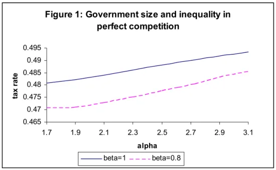
experimentation with empirically relevant parameter values (which also satisfy the second-order conditions and inequality (17)), we find that increases in inequality result in smaller tax rates (albeit the effect is rather small). Following Creedy (1977), we run our simulations for values of a that range between 1.7 and 3.0. In order to keep average income constant as a increases, we set b=µ(a−1)/a for various values ofµ. Figure 1 displays the median voter’s preferred tax rates (size of government) as a function of inequality (higher values of

α imply lower inequality) and for two values of the parameter measuring the efficiency difference between the private and the public sector ( β =0.8 and β =1). As expected, the

lower is the efficiency of the public sector the lower is the tax rate, since in this case the cost of expanding public sector production at the expense of the private sector is higher6. Note that the results depicted in figure 1 do not depend on the level of µ: The relationship

between the tax rate and inequality remains -ceteris paribus- qualitatively similar at any level of average income.

Figure 1: Government size and inequality in perfect competition 0.465 0.47 0.475 0.48 0.485 0.49 0.495 1.7 1.9 2.1 2.3 2.5 2.7 2.9 3.1 alpha tax rate beta=1 beta=0.8

The explanation for the – opposite to the literature - result that increases in equality result in

a higher tax rate relies on the fact that the median voter in the present model must weigh the impact of two effects as she contemplates a rise in the tax rate in response to an increase in inequality. The first one is the traditional effect identified in the literature which leads to an increase in the tax rate preferred by the median voter as the gap between mean and median (pre-tax) income increases – since the median voter expects that a rise in the tax rate will bring to her a greater increase in public goods provision than before. But in addition to this,

the median voter in the present paper must also take into account that a higher tax rate will induce some high-income households to switch their demand from a privately supplied variety to the publicly supplied. Accordingly, the government may not be able to use the increased tax revenue to produce a variety of higher quality as it will have to provide the good to a higher number of households. It is thus by no means certain that a higher tax rate will procure the median voter (and everyone else) a higher quality of the public good. Our numerical results show that from the two effects mentioned the second tends to dominate the first, thus producing a small negative effect of inequality on the tax rate (size of

government)7.

The absence of a non-monotonic relationship between the tax rate and the quality of the publicly provided variety – due to the endogeneity of the proportion of households

consuming this variety - is also verified by our numerical results. We find that starting from a low level of a, although increases in equality produce a monotonic increase in tax rates, they result initially in decreases in the quality of the publicly provided variety and then in higher increases it (thus producing a U-shaped relationship between equality and the quality

7 _{It is worth mentioning that in case the government was not involved in producing the vertically-differentiated}

product (and providing it freely to all those wishing to consume the publicly-provided variety), but was instead returning the tax proceeds in a lump-sum way to every household, then the median voter would prefer a tax rate equal to 100%. This is, of course, due to our assumption that there are no-disincentive effects of higher taxes in our model (see, Harms and Zink (2003) for a review of theories suggesting mechanisms leadind to limited redistribution). In this sense public provision of private goods may be a relatively inexpensive way for high-income individuals to avoid expropriation by the poor ( Roemer (1998) suggests an alternative way to avoid such expropriation, namely increasing the salience of some non-economic issues ). In a fuller model, the mode of redistribution would itself be endogenous - thus enhancing the role of the agenda setting institutions in modern democracies (see, Persson and Tabellini (2003) for an empirical analysis of modes of governance).

of publicly provided services). This is explained by the fact that a change in the inequality parameter changes the proportion of households belonging to a given interval of the income distribution, thus altering the number of households that choose to consume the publicly-provided variety as the tax rate changes.

4. Monopoly

We now assume that the vertically-differentiated product is produced under imperfectly competitive conditions. For goods like health care and education, the assumption of

imperfect competition is most likely a better approximation of reality than the assumption of perfect competition. In the same vein, the assumption of monopoly is a less suitable

approximation of reality than other imperfectly competitive structures.Nevertheless, we present here the case of monopoly since, in addition to being the polar opposite of perfect competition, is both analytically simpler than other imperfectly competitive market structures, and itproduces results whose nature is similar to, for example, an oligopolistic market structure. In order to avoid unnecessary complications regarding the nature of the political equilibrium (which would not help in comparing this case with the perfectly competitive one), we assume that this is a foreign owned monopoly – so that its owners are not citizens of the home country and thus do not have voting rights. Moreover we assume that the profits accruing to the foreign owners are not taxed.

Unlike the perfectly competitive case, in which the price of each variety was equal to the cost of producing it, the monopolist will choose a price-quality combination which maximizes its profits. We assume that the monopolist will set a single price-quality combination.

Nevertheless, the presence of a publicly-provided variety creates a constraint (in effect defines the “demand curve”) for the monopolist. As previously, let _θM _{stand for the level of}

(pre-tax) income that makes a household indifferent between consuming the publicly-provided variety (_QG_{) and the variety offered by the monopolist (Q}M_{) at the price P}M_{, i.e.}

(

(1 )

)

(1 )

P M M M G M G

V

=

Q

θ

− −

t

P

=

Q

θ

− =

t

V

. (20) Thus,

/(1 )(

)

M

P Q

M M

t Q

M

Q

G

θ

=

−

−

(21) Equation (21) implicitly defines the proportion of households (₌( /_b

θ

M)α_{) which will}

choose to pay the price charged by the monopolist in order to avail themselves of the higher-quality variety offered by the monopolist. Thus, the monopolist sets _PM _{and Q}M _{so as to}

,

max

(

)( /

)

M M M M M P Q

P

Q

b

α

β

θ

Π =

−

,

subject to the constraint provided by equation (21). The first-order-conditions imply that

1 M M P =

α

α β

Q − (22) 2 1 1 M G Q

α

Q

α

− = − . (23)

Equation (22) implies that the mark-up of price (PM) over cost (=

β

QM) depends only on the (in)equality parameter

α

. The higher is inequality, the higher is the mark-up. Using equations (22), (23) and (21) we find that

2 2

(2

1)

(1 )(

1)

M

Q

G

t

β α

θ

α

−

=

−

−

. (24)

In effect, equation (24) informs the median voter how her choice of the tax rate and of the quality of the publicly-provided good (which will be implemented by the policy maker) affects the proportion of households which will be consuming the variety provided by the monopolist. It thus summarizes for the median voter the effects of her current policy choices on the future behavior of the monopolist, which she takes into account when deciding – in

that even though –in equilibrium - the median voter will not be consuming the variety offered by the monopolist, she must, nevertheless, take into account the monopolist’s actions since these actions affect the proportion of households consuming the publicly-provided variety, and thus, through the government budget constraint, the feasibility of her choices. As explained in the previous section, the tax rate (and the associated publicly-provided variety,

*G

Q ) preferred by the median voter will be positive only if at this tax rate (_t*_{) the resulting}

utility for the median voter is higher than that which the median voter would attain if the tax rate was zero and was consuming the variety offered by the monopolist, i.e.

* * 1/ 1/ * , * , 0 , G

2 (1

)

( 2 ) M M Q G G P m t m t

b

t Q

Q

b P

V

α α

V

= −

−

=

>

=

. (25)

Assuming that this condition is satisfied – this is further discussed in the following paragraphs – we conceive that the median voter solves the following program, i.e.

, 1/

max

_G

2 (1 )

G t Q

U

b

t Q

α

=

−

,

subject to the government budget constraint (equation (14)) and equation (24). This maximization implies that

* * * * 2 2 2

(

1)

((2

1) (

)

(

1) ( (1 )) )

(

) (2

1)

G G G

Q

a

Q

a

b

t

t

b

Q

a

α α α α α α

α

β

α β

−

−

− −

−

=

−

(26) * * * 1/( 1) 2 1 2

2(

1)

( (1

))

(1 2 )

(2

1)

G

b

t

Q

b

t

α α α α α

α

β

α

− +        

−

−

=

−

−

(27)

Equations (22), (23), (24), (26) and (27) determine the values of _{t Q}*_, *G_,

θ

M_,PM_{and Q}M _. As in the perfectly competitive case, the comparative statics effects of changes in the

in(equality) parameter α are, in general, ambiguous. However, after extensive

experimentation with empirically relevant parameter values (which also satisfy the second-order conditions and inequality (25)), we find that increases in equality (rises in parameter

α

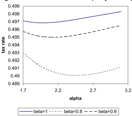
) initially result in (small) reductions in the tax rate, which are later reversed, thus producing an almost U-shaped relationship between equality and the tax rate. Figure 2 displays this relationship for three different values of

β

(the parameter measuring the efficiency difference between the private and the public sector). The choice of parameter values in our simulations is the same as in the case of perfect competition. Again, a change in average income has no impact on the relationship between inequality and the tax rate. As expected, the lower is

β

, the lower is –ceteris paribus- the tax rate (and the quality of the publicly-provided variety).

Figure 2: Government size and inequality in monopoly

0.489 0.49 0.491 0.492 0.493 0.494 0.495 0.496 0.497 0.498 0.499 1.7 2.2 2.7 3.2 alpha tax r a te

beta=1 beta=0.8 beta=0.6

Comparing Figures 1 and 2 we see that the tax rate chosen by the median voter is higher in the case of monopoly8. This is understandable since the presence of monopoly is expected to

lead –ceteris paribus- to a larger proportion of households choosing to consume the publicly-provided variety (than in the perfectly competitive case) because the monopolist charges a price larger than cost. This implies that the median voter expects that any given rise in the tax rate (which increases the sum available for redistribution) will add a smaller number of households to those already consuming the publicly-provided variety (QG) in the monopoly case, since the income distribution is thinning at its tails. Consequently, the median voter will be expecting a larger rise in QG than the increase in government revenue effects in the monopoly case, and thus she will be willing to vote for a higher tax rate than in the competitive case. One can also note that as inequality decreases (parameter

α

rises) the impact of inequality on the tax rate becomes similar in the monopoly and perfectly

competitive cases. This is not surprising since as one can see from equation (22), an increase in parameter

α

shrinks the monopoly mark-up of price over cost, so that the difference between monopolistic and perfectly competitive behaviour becomes less significant.

Finally, it is interesting to compare the political equilibrium conditions for a positive tax rate under perfect competition and under monopoly. One can see from conditions (17) and (20) that the median voter’s net utility gain from a positive tax in equilibrium decreases as the efficiency difference between the public and the private sector increases (parameter

β

).9 Moreover, the value of

β

at which the median voter is indifferent between public

consumption and private consumption (with zero tax rate) is lower for the monopoly case. This implies that the monopolistic setting preserves a positive tax rate in equilibrium even though the efficiency difference between the private and the public sector would induce the median voter to vote for a zero tax rate if the private sector was competitive. It thus appears that the median voter chooses to “counteract” the monopolist’s power by voting for a public provision of the VDP, even if this entails shifting production to a less efficient “producer”.

5. Conclusion

In this paper we consider what happens if the government can redistribute through both sides of its budget (revenue and expenditure). We model this by introducing the possibility that

high-income individuals may decide not to ″_{consume” what the government is offering as a}

public good to all citizens. We find that changes in inequality do not have an unambiguous effect on the size of government. Our simulation results suggest that this effect will depend on the market structure for the vertically-differentiated product. Under perfect competition the relationship between equilibrium tax rate and equality is positive while the relationship becomes U-shaped under monopoly. Moreover, the assumption of a monopolistic structure in the production of the vertically-differentiated good has two important consequences for the size of the public sector: Firstly, we find a monopoly bias in the size of government in the sense that under monopoly the median voter will vote for a higher tax rate. Secondly, the presence of monopoly induces the median voter to be in favour of public provision of private goods (a positive tax rate), even in cases in which the public sector is so inefficient that under perfectly competitive conditions the political equilibrium would not be supportive of any positive tax rate.

References

Alesina, A. and D. Rodrik (1994), “Distributive politics and economic growth”, Quarterly Journal of Econmics,109, pp. 465-490.

Alesina, A., E. Glaeser, and B. Sacerdote (2001),“Why doesn’t the US have a European-style welfare system”, Brookings Papers on Economic Activity, pp. 187-278.

Benabou, R. (1996) “Inequality and growth”, in R. Bernanke and J. Rotemberg, (eds.), NBER Macroeconomics Annual, 11-74, NBER, Cambridge, Mass.

Benabou, R. (2000), “Unequal societies: Income distribution and the social contract”, American Economic Review, 90, pp. 96-129.

Besley, T. and S. Coate (1991), “Public provision of public goods and the redistribution of income”,

American Economic Review, 81, pp. 979-984.

Blomquist, S. and V. Christiansen (1995), "Public Provision of Private Goods as a Redistributive Device in an Optimum Tax Model", Scandinavian Journal of Economics, 97, pp. 547-567. Blomquist, S. and V. Christiansen (1999), "The Political Economy of Publicly Provided Private Goods", Journal of Public Economics, 73, pp. 31-54.

Boadway, R. and M. Marchand (1995), "The Use of Public Expenditures for Redistributive Purposes", Oxford Economic Papers, 47, pp. 45-59.

Clarke, G.R.C. (1995), “More evidence on income distribution and growth”, Journal of Developmant Economics, 47, pp. 403-427.

Creedy, J. (1977), “Pareto and the distribution of income,” Review of Income and Wealth, 23, pp. 405-411.

Flam, H. and E. Helpman, (1987), “Vertical product differentiation and North-South trade”, American Economic Review, 77, pp. 810-822.

Grandmont, J.-M. (1978), “ Intermediate Preferences and the Majority Rule”, Econometrica, 46, pp. 317-330.

Grossmann, V. (2003), “Income inequality, voting over the size of public consumption, and growth”,

European Journal of Political Economy, 19, pp. 265-287.

Harms, P. and S. Zink (2003), “Limits to redistribution in a democracy: a survey”, European Journal of Political Economy 19, pp. 651-668.

Lee, W. and J. Roemer (1999),“Inequality and redistribution revisited”, Economics Letters, 65, pp. 339-346.

Meltzer, A. and S. Richard (1981), “A rational theory of the size of government”, Journal of Political Economy, 89, pp. 914-27.

Meltzer, A. and S. Richard, (1983),“Tests of a rational theory of the size of government”, Public Choice, 41, pp. 403-18.

Milanovic, B. (2000), “The median-voter hypothesis, income inequality, and income redistribution: an empirical test with the required data”, European Journal of Political Economy, 16, pp. 367-410. Munro, A. (1991), "The Optimal Public Provision of Private Goods", Journal of Public Economics,

44, pp. 239-261.

Persson, T. and G. Tabellini (1994), “Is inequality harmful for growth?”, American Economic Review, 84, pp. 600-621.

Persson, T. and G. Tabellini (2000), Political Economics:Explaining Economic Policy, The MIT Press.

Persson, T. and G. Tabellini (2003), The Economic Effects of Constitutions, The MIT Press. Rodriguez, F.C. (1999), “Does distributional skewness lead to redistribution? Evidence from the

Roemer, J. (1998), “Why the poor do not expropriate the rich: an old argument in new garb”, Journal of Public Economics, 70, pp. 399-424.

Romer, T. (1975), "Individual Welfare, Majority Voting, and the Properties of a Linear Income Tax",

Journal of Public Economics, 7, pp. 163-185.

Rosen, S. (1974), "Hedonic Prices and Implicit Markets: Product Differentiation in Pure Competition”, Journal of Political Economy, 82, pp. 34-55.

Saint-Paul, G. (2001), “The dynamics of exclusion and fiscal conservatism”, Review of Economic Dynamics, 4, pp. 275-302.

Thum, C. and M. Thum (2001), "Repeated Interaction and the Public Provision of Private Goods",

Scandinavian Journal of Economics, 103, pp. 625-643.