Model based control charts
in stage 1 quality control
Alex J. Koning
Econometric Institute Erasmus University Rotterdam
P.O. Box 1738 NL-3000 DR Rotterdam
The Netherlands
Econometric Institute Report EI-9958/A
Abstract
In this paper a general method of constructing control charts for preliminary analysis of individual observations is presented, which is based on recursive score residuals. A simulation study shows that cer-tain implementations of these charts are highly effective in detecting assignable causes.
Key Words: Cusum chart, control chart, statistical process control.
Introduction
When a process is new or just has been modified, one is faced with two seperate problems. Firstly, it is unknown whether the process is in-control; secondly, the parameters governing the in-control statistical behavior of the process are unknown. Stage 1 quality control aims at solving both problems simultaneously on the basis of historical data. If stage 1 qual-ity control yields the conclusion that the process is indeed in-control, then stage 1 is followed by stage 2 quality control. Stage 2 quality control aims at detecting departures from the control state on the basis of the in-control parameter estimates obtained in stage 1 and prospective data.
Additional information concerning stage 1 and stage 2 quality control may be found in the introduction in Sullivan and Woodall (1996) and the introduction in Koning and Does (1999). In Sullivan and Woodall (1996) the importance of the detection of assignable causes is emphasized. In
Koning and Does (1999) the relevance of stage 1 quality control for current manufacturing processes is underlined.
Stage 1 quality control relies heavily on control charts, which often are constructed following either the likelihood ratio approach or the recursive residual approach.
In the likelihood ratio approach [cf. Quandt (1960), Hinkley (1971), Worsley (1986), Sullivan and Woodall (1996)] the full sample of historical dataX
1
;:::;X
nis divided into two subsamples X 1 ;:::;X kand X k+1 ;:::;X n,
and these two subsamples are compared by computing a two-sample like-lihood ratio test statistic
k under the given model. The procedure is
re-peated for every 1 k < n, and
k is plotted is versus
k. Finally, a
hor-izontal decision line is added to the chart and used to asses whether the process may be classified as being in-control.
In the recursive residuals approach [Brown, Durbin and Evans (1975), Hawkins (1987), Quesenberry (1991, 1995), Del Castillo and Montgomery (1994), Koning and Does (1999), Koning (1999)] the unknown in-control pa-rameters are eliminated by cleverly transforming the historical data so as to obtain a number of independent random variables which have distribu-tions [virtually] not depending on the unknown in-control parameters but reacting to out-of-control conditions nevertheless. The transformed data are used to asses whether the original data are in-control. In Koning and Does (1999) and Koning (1999) the recursive residual approach is combined with the theory of uniformly most powerful tests [cf. Lehmann (1994)] so as to obtain control charts which are optimal for detecting a particular form of trend in normally distributed random variables. The chart proposed in Koning and Does (1999), which was developed for detecting linear trend in normally distributed random variables, showed the best properties to detect linear trends and shifts in the data in a comparison with various other charts [including the LRT-chart of Sullivan and Woodall (1996) and the Cusum chart of Brown, Durbin and Evans (1975)].
The “recursive residuals” literature mentioned above concentrates on the situation where the observations follow a normal distribution. In con-trast to the likelihood ratio approach there is no obvious extension of the recursive residual approach to the nonnormal situations. However, in this paper a possible way of extending the recursive residual approach to non-normal situations is presented.
The structure of this paper is as follows. First, we introduce the concept of recursive score residuals, which form the basis of the extension of the recursive residual approach to nonnormal situations. After describing how recursive score residual arise naturally in detecting assignable causes in exponential families, we generalize to distributions which do not necessar-ily belong to an exponential famnecessar-ily, and discuss several ways of implement-ing the charts. Finally, we focus on the normal distribution to select an
implementation which is highly effective according to simulation results, and apply this implementation to the data sets in Sullivan and Woodall (1996).
Recursive score residuals
In this section we introduce the concept of recursive score residuals, which will allow us to extend the recursive residual approach to nonnormal situ-ations.
Let the random variableX have density function f(x;), where the
pa-rameter belongs to some parameter space IR k
. Define the classical score function by
(x;)= @ @
logf(x;):
Note that is a vector-valued function, of the same dimension k as the
parameter.
The individual score (X;) is obtained by transforming the random
variableXvia the classical score function. It is well-known that the
math-ematical expectationE
(X;)is equal to zero; moreover, if thekk Fisher
information matrixexists, then
E
(X;)(X;) T
=
[cf. Section 5.1.2 in Lindsey (1996)]. Recall that the Fisher information matrix depends on.
Now, consider the situation in which we have observed n independent
copiesX 1 ;:::;X n of X. Define Y i = s i 1 i 8 < : (X i ;) 1 i 1 i 1 X j=1 (X j ;) 9 = ; :
One may viewY
ias a recursive residual formed from the individual scores.
We shall refer to Y
i as the i
th
recursive score residual. Note that Y 1 is
degenerate in zero, and hence does not convey any information whatsoever. Thus, it suffices to only considerY
2 ;:::;Y
n.
It is easily seen thatE
Y i
=0. Moreover, one may show that
E Y i Y T j = ( ifi=j >1; 0 ifi6=j;
Thus, the recursive score residualsY 2
;:::;Y
nhave expectation zero,
covari-ancematrixand are uncorrelated. Note that being uncorrelated does not
Recursive score residuals in exponential
fam-ilies
A random variableXis said to belong to an exponential family if its density
function admits the representation
f(x;)=c()h(x)exp n () T t(x) o (1)
[cf. Lehmann (1994), Section 2.7]. If in addition the dimension of the vector
()coincides with the dimension of, then the random variable X is said
to belong to a full exponential family. In Section 6.2 of Hawkins and Olwell (1998) the relevance of exponential families for statistical quality control is discussed, and examples are given.
It is often convenient to reparametrize a full exponential family by tak-ing = () as parameter instead of. In this way we obtain the natural
or canonical reparametrization in whichX has density function
f (x;)=c ()h(x)exp n T t(x) o ; wherec () satisfies c (()) = c(). Let
(x;) denote the classical score
function derived under the natural parametrization. One may show that
(x;)= @ @ logf (x;)=t(x) E t(X)
[see Equation (3.106) in Lindsey (1996), p. 124]. Hence, it follows that the
i th
“natural” recursive score residual is given by
Y i = s i 1 i 8 < : t(X i ) 1 i 1 i 1 X j=1 t(X j ) 9 = ; : Note thatY i
does not depend on.
The reparametrization above was introduced because of its technical convenience. However, in stage 1 quality control the original parametriza-tion may be carefully chosen so as to optimize the detecparametriza-tion of assignable causes, and reparametrization should be avoided. Fortunately, thei
th
“orig-inal” recursive score residual Y
i are easily derived from the i
th
“natural” recursive score residualY
i
. Since differentiating via the chain rule yields
(x;)= (x;()) @() @ ;
it immediately follows that
Y i =Y i @() @ :
Note that @()=@ is a k k matrix, possibly depending on . Also note
that the Fisher information matrixin the original parametrization takes
the form = @() @ @() @ ! T ; where
is the Fisher information matrix in the canonical parametriza-tion.
Detecting assignable causes: exponential
fam-ilies
In this section we consider independent random variablesX 1 ;:::;X n with X i having density f(x; i
)which can be written in the form (1).
Note that the situation considered in the previous section is obtained by setting all
i’s equal to
, and corresponds to a process which is in-control.
The situation in this section also allows for
i’s not sharing the same value,
corresponding to a process which is not in-control. Let us suppose that the
i’s satisfy ( i )= +Æa i d; (2)
where Æ is a scalar representing the magnitude of the deviation between (
i
) and ,
a
i is a scalar representing the type of deviation [sudden shift,
linear trend, etcetera], and d is a k-dimensional vector representing the
direction of the deviation. Observe that the process is in-control if and only if the(
i
)’s admit a representation (2) withÆ equal to zero.
The joint density ofX 1
;:::;X
nmay now be written in the form
c(Æ;a 1 ;:::;a n ;d)h(x 1 ;:::;x n )exp 8 < : T n X j=1 t(x j )+Æ n X j=1 a j d T t(x j ) 9 = ; :
It follows from Corollary 2 in Chapter 3 of Lehmann (1994) that the test statistic n X j=1 f( 0 )+a i dg T t(X j ) (3)
is most powerful for testing the simple null hypothesisH 0 : ( 1 ) = = ( n ) =
0 versus the alternative described by (2). Moreover, in the
in-control situation the statistic P n j=1 t(X j ) is sufficient for , the common value of the ( i
)’s [Lehmann (1994), p.57]. Now note that the null
in-control sufficient statisticP n j=1 t(X j )is equal to n X j=1 f( 0 )+a j dg T Et(X 1 ) T t(X 1 );
which becomes zero when
0 equals +a n d, where a n denotes n 1 P n j=1 a j.
One may interpret this particular value of
0 as some sort of a “least
favor-able” null parameter1 in the sense of H ´ajek and ˇSid ´ak (1967), p. 30. Note
that substituting
+a n
dfor
0 in (3) yields the test statistic n X j=1 (a j a n )d T t(X j ):
Hence, this test statistic [which does not depend onÆ] should be highly
effi-cient in testing the composite null hypothesis that all
i’s are equal versus
the alternative described by (2).
By letting the directiondvary, it follows that plots of the components of
thek-dimensional vectorU
i defined by U i = i X j=1 (a j a i )t(X j )
may be highly effective in detecting out-of-control behavior of the type de-scribed bya
1 ;:::;a
n. Note that U
1 is degenerate in zero. Moreover, since we
have U i U i 1 = i X j=1 (a j a i )t(X j ) i 1 X j=1 (a j a i 1 )t(X j ) = (a i a i )t(X i ) ( a i a i 1 ) i 1 X j=1 t(X j ) = (a i a i ) 8 < : t(X i ) 1 i 1 i 1 X j=1 t(X j ) 9 = ; = (a i a i ) s i i 1 Y i = (a i a i 1 ) s i 1 i Y i ;
we may alternatively express U
i in terms of the natural recursive score
residualsY 1 ;:::;Y i as U i = i X j=2 c i Y j ; (4)
1According to H ´ajek and ˇSid ´ak (1967) the most powerful test statistic and the
suffi-cient statistic should be independent for the least favorable null parameter. Recall that independence implies zero covariance, but not vice-versa.
where c i =(a i a i 1 ) s i 1 i : (5)
We defer the precise description of the chart based on theU
i’s to the end
of the next section.
Detecting assignable causes: the general case
In this section we consider independent random variablesX 1 ;:::;X n with X i having density f(x; i
), not necessarily belonging to an exponential
fam-ily.
In exponential families we were able to exploit the special structure of the natural classical score function, which may be viewed as the difference between a term depending only on x and a term only depending on the
parameter. Such a structure is in the general case not available.
However, if we are willing to assume that all
i’s are relatively close to
the in-control parameter , then locally around the classical score
func-tion approximately has the structure encountered in exponential families, provided that the approximation
(x;#)(x;) (# ) (6)
holds for every # in the vicinity of . As before, denotes the in-control
Fisher information. In the stage 2 quality control context, a similar ap-proximation may be found in Box and Ramirez (1992).
In exponential families we were also able to exploit the theory of most powerful tests in order to construct test statistics. In the general case we have to resort to asymptotic efficiency concepts and intuitions gained in the previous section.
We start with observing that (6) implies the approximation
Y i s i 1 i 0 @ i 1 i 1 i 1 X j=1 j 1 A +W i ; (7) where W i = s i 1 i 8 < : (x i ; i ) 1 i 1 i 1 X j=1 (x j ; j ) 9 = ; : Since E i (X i ; i
) = 0 for every i = 1;1;:::;n, the random variable W i has
mathematical expectation equal to zero, which coincides with the in-control expectation ofY i. Moreover, for i close to we have E i (X i ; i )(X i ; i ) T ;
hence, if 1
;:::;
i are all close to
, then the random variable W
i
approxi-mately has covariance matrix , the in-control covariance matrix of Y i. In
a similar way we may show thatW i and
W
j are uncorrelated if
i6=j. Thus,
the behavior of the sequenceW 2
;:::;W
n approximately is the same as the
in-control behavior of the sequence Y 2
;:::;Y
n, as far as first and second
moments are concerned. In combination with (7) this leads us to the con-clusion that the main effect of the transition from the in-control situation to the present situation is a shift in the distribution of the Y
i’s. We shall
refer to this shift as the slope of the test statisticY i.
Suppose that the
i’s in fact satisfy i = +Æa i d;
where as before Æ is a scalar representing the magnitude of the deviation
between i and
,
a
i is a scalar representing the type of deviation, and d is a k-dimensional vector representing the direction of the deviation. It
follows from (7) that the slope ofY
i is approximately s i 1 i 0 @ i 1 i 1 i 1 X j=1 j 1 A =Æ s i 1 i (a i a i 1 )d=Æc i d; andc i is given by (5).
In the previous section we found that linear combinations of the Y i’s
were most powerful. This leads us now to concentrate on the performance of linear combinations P n i=2 w T i Y
i as test statistics when testing the null
hypothesis H 0
: Æ = 0 versus a one-sided alternative. Here the w i’s are
given k-dimensional weight vectors, for which we shall derive an optimal
choice shortly.
Various efficiency concepts suggest that efficiency of a test statistic is indicated by the ratio between the its squared slope and its null-hypothesis variance [see Kallenberg and Koning (1995)]. Straightforward calculations show that the variance ofP
n i=2 w T i Y
iis approximately equal to the in-control
variance P n i=2 w T i w
i. Moreover, the slope of P n i=2 w T i Y i is approximately equal to Æ n X i=2 c i w T i d:
Thus, the eficiency of linear combinationsP n i=2 w T i Y
i is indicated by the
ra-tio n X i=2 c i w T i d ! 2 P n i=2 w T i w i :
An application of the Inequality of Cauchy-Schwarz yields that this ratio is maximized by choosingw
i proportional to c
i
d T U i, where U i = i X j=2 c i Y j [compare with (4)]. Observe thatU
i approximately has mathematical expectation Æ P i j=2 c 2 j d T d and variance P i j=2 c 2 j d T
d. Thus, both the expectation and the
vari-ance of U
i are approximately linear in P i j=2 c 2 j
, which indicates that U i
should be plotted versus P i j=2
c 2
j rather than versus
i itself. A disturbing
consequence is that [in contrast to traditional cumulative sums] the time instanceP n j=2 c 2 j
at which the “last” observation in the sample is observed, does not depend linearly on the sample size anymore. This can be repaired by introducing b n = 0 @ n 1 n X j=2 c 2 j 1 A 1=2 ; (8)
and plotting the cumulative sumb n U i versus b 2 n P i j=2 c 2 j . Moreover, since a nonzero value ofÆ approximately corresponds to a linear trend in the plot
of b n U i versus b 2 n P i j=2 c 2 j
, applying a V-mask procedure to this plot seems reasonable.
It was shown in Lucas (1982) [cf. Montgomery (1996)] that a V-mask cumulative sum chart may be represented by means of a pair of so-called tabular cumulative sums. Following the same line of reasoning, one may show that the V-mask procedure applied to the plot ofb
n U iversus b 2 n P i j=2 c 2 j
is equivalent to imposing a control limithon the pair of one-sided
cumula-tive sumsC H ;iand C L;idefined by C H ;i =max(0;C H ;i 1 +b n c i (Y i fb n c i )); C L;i =max(0;C L;i 1 +b n c i ( Y i fb n c i )); (9)
where f is the so-called reference value. Observe that both C
H ;i and C
L;i
are k-dimensional random vectors; the control limit h should be imposed
on all components of these random variables simultaneously. That is, an out-of-control signal is given when at least one of these components exceeds
h.
Implementing the charts
In the previous sections we presented the general ideas behind the pro-posed charts, ideas that give the charts the ability to detect the assignable cause efficiently. However, until now we have avoided technical issues that
emerge when implementing the charts. In this section we discuss these issues and offer some solutions.
The first technical issue concerns the dependence between the compo-nents ofU
i. Earlier, we suggested to plot components of U i versus an appro-priate time-scaleP i j=2 c 2
j. Due to the fact that the covariance matrix of U
iis
approximately proportional to the in-control Fisher information, it may
be that the components ofU
i are highly correlated, which makes it difficult
to identify the precise nature of the assignable cause when detected. To avoid this, we should look at the components of
1=2 U irather than U i itself; here 1=2
denotes a matrix such that 1=2
1=2
is the identity matrix for some matrix
1=2 which satisfies 1=2 ( 1=2 ) T = . In general, several choices of 1=2
are available. For instance, one may obtain a matrix 1=2
as a result of inverting the LU-root of; this would be appropriate if the
components of could be ranked according to importance. Alternatively,
one may set 1=2
equal toR D 1=2
R T
, whereDis a diagonal matrix andR
is a rotation matrix satisfying R DR T
= ; this may be appropriate if the
components ofdo not differ in importance.
The second technical issue concerns the computation of the in-control Fisher information matrix . It may well be that the computation of
becomes too intricate. An alternative is to estimate from the data. One
may estimateby 1 n n X j=1 (X j ;)(X j ;) T : (10)
The third technical issue concerns the fact thatY i,
and estimators of may depend on the unknown in-control parameter . One may resolve
this issue by replacing occurrences of by occurrences of ^
n, where ^ is a
full sample estimator of . If ^
n takes values close to
, it should be noted
that by virtue of (6) we have
s i 1 i 8 < : (X i ; ^ n ) 1 i 1 i 1 X j=1 (X j ; ^ n ) 9 = ; Y i + s i 1 i 0 @ ( ^ n ) 1 i 1 i 1 X j=1 ( ^ n ) 9 = ; =Y i :
As remarked earlier, in exponential families the natural recursive score residualY
i
does not depend on.
The fourth technical issue concerns the choice between full-sample and “running” estimators. Above, we have proposed using full sample estima-tors to estimate and , as they are the most obvious estimators under
in-control conditions. Unfortunately, there is a practical drawback: the use of full sample estimators introduces a masking effect, since out-of-control conditions may inflate full sample estimators.
To avoid the drawback of full sample estimation, one may instead use “running” estimation. Rewrite
1=2 U i in the form i X j=2 c j 1=2 Y j ;
and replace every occurence of in 1=2 Y j by ^ j 1, an estimator solely
based on the firstj 1observationsX 1
;:::;X
j 1. If desired, one may first
estimateby (10), withn replaced byi 1.
Although running estimation does not suffer from the masking effect, it has a drawback of its own. Especially early in the sequence, the variability of the running estimators may lead to “estimated” recursive score residuals with extremely heavy tails. To remedy this, one may consider the use of transformations along the lines of Hawkins (1987) and Quesenberry (1991, 1995). However, such transformations may in turn depend on the unknown in-control parameter; estimating this parameter may produce estimated
recursive score residuals which have correlated components.
The fifth technical issue concerns the method of estimating. Since the
classical score function already belongs to the realm of likelihood, it seems natural to use maximum likelihood estimator. The full sample maximum likelihood estimator ^
ML
n
is found by solving the likelihood equations
n X j=1 (X i ; ^ ML n )=0: (11)
When replacingnbyi 1in (11) one obtains the maximum likehood
equa-tions for the running maximum likelihood estimator ^
ML
i 1
. Observe that these “running” likelihood equations directly imply that
s i 1 i 8 < : (X i ; ^ ML i 1 ) 1 i 1 i 1 X j=1 (X j ; ^ ML i 1 ) 9 = ; = s i 1 i (X i ; ^ ML i 1 );
which underlines the naturalness of maximum likelihood estimation in the presence of classical score functions.
The sixth and final technical issue concerns time reversal. Although the proposed charts were developed to detect a particular assignable cause, they are typically higly effective in detecting other assignable causes as well. For instance, the chart for detecting linear trend is also sensitive to sudden shifts occurring not too early in the sample. Reversing time yields other charts, with “secundary” properties that may be favourable: the “reversed time” chart for detecting linear trend is sensitive to sudden shifts occurring not too late in the sample.
Detecting linear trend in normal quality
char-acteristics
In this section we exemplify the methods discussed previously by apply-ing them to the problem of detectapply-ing linear trend in quality characteristics which follow a normal distribution. The in-control parametersand
2
are unknown.
The in-control density of these quality characteristics is given by
f(x;; 2 )= 1 p 2 2 exp ( 1 2 (x ) 2 2 ) ;
which can be written in exponential form as
f(x;; 2 )= 1 p 2 2 exp ( 2 2 2 ) exp n (; 2 ) T t(x) o with (; 2 )= 2 1 2 2 ! ; t(x)= x x 2 ! :
Let denote the vector (; 2
) T
, and let X a random variable with density f(x;; 2 ). Since E t(X)= 2 + 2 ! ;
it follows that the natural classical score function is given by
(x;; 2 )= x x 2 (+ 2 ) ! : Moreover, since @() @ = 1 2 0 4 1 2 4 ! ;
it follows that the original classical score function is given by
(x;; 2 )= x x 2 (+ 2 ) ! 1 2 0 4 1 2 4 ! = 1 2 x 1 2 (x ) 2 2 1 ! :
Alternatively, we could have obtained the original classical score function by directly differentiating logf(x;; 2 )= 1 2 log2 1 2 log 2 1 2 (x ) 2 2
with respect toand 2
It is now easily derived that Y i = s i 1 i 1 2 0 @ X i 1 i 1 P i 1 j=1 X j 1 2 n (X i ) 2 2 1 i 1 P i 1 j=1 (Xj ) 2 2 o 1 A :
The in-control Fisher information, the in-control covariance matrix ofY i, is given by = 1 2 0 0 1 2 4 ! :
Since happens to be a diagonal matrix, the issue of choosing 1=2
does not emerge here. The only available choice is
1=2 = 0 0 2 p 2 ! : Thus, we obtain 1=2 Y i = s i 1 i 0 @ 1 n X i 1 i 1 P i 1 j=1 X j o 1 2 p 2 n (X i ) 2 1 i 1 P i 1 j=1 (X j ) 2 o 1 A : (12) Note that 1=2 Y
i depends on the unknown in-control parameters
and 2
. Replacing these unknown values by their full sample estimators
X n = 1 n n X j=1 X j and S 2 n = 1 n 1 n X j=1 (X j X n ) 2 yields Z n;i = s i 1 i 0 @ 1 S n n X i 1 i 1 P i 1 j=1 X j o 1 S 2 n p 2 n (X i X n ) 2 1 i 1 P i 1 j=1 (X j X n ) 2 o 1 A as an approximation to 1=2 Y
i. Observe that each of the Z
n;i’s has the same
distribution.
To derive charts for detecting linear trend, we should set a
i equal to i,
which yields that the tabular Cusum scheme (9) should be applied with
c i = s i 1 i (a i a i 1 )= s i 1 i (i i=2)= q (i 1)i=2 andY i replaced by Z
n;i. Note that considering only the first components of C
H ;iand C
L;ileads to the Cusum chart proposed in Koning and Does (1999).
Replacing the unknown in-control parameters and 2 their running estimators X i 1 and S 2 i 1 yields Z i 1;i = s i 1 i 0 B @ X i X i 1 =S i 1 1 p 2 X i X i 1 =S i 1 2 1 1 C A
as an approximation to 1=2 Y i. Observe that Z 2;3 ;Z 3;4 ;:::;Z n 1;n remain
uncorrelated, but have widely varying in-control behavior: one may con-sider Z i 1;i to be a function of q (i 1)=i(X i X i 1 )=S i 1, which has a t
-distribution withi 1degrees of freedom. It is well-known that the
heavy-tailed Cauchy distribution is a special case of the t-distribution, and the
light-tailed normal distribution is a limiting case. To remedy the varying behavior we could consider replacing
q (i 1)=i(X i X i 1 )=S i 1 by Q i = 1 0 @ G i 1 0 @ s i 1 i 0 @ X i 1 i 1 i 1 X j=1 X j 1 A =S i 1 1 A 1 A ; where 1
denotes the standard normal inverse cumulative distribution function, and G
i 1 the cumulative distribution function belonging to the t-distribution with i 1 degrees of freedom. In Quesenberry (1991) it is
shown thatQ 3
;:::;Q
n are independent random variables under in-control
conditions. Using theQ
i’s as replacements leads to Z i 1;i = Q i 1 p 2 q i i 1 Q 2 i 1 ! as an approximation to 1=2 Y
i. To derive charts for detecting linear trend,
the tabular Cusum scheme (9) should be applied withY
i replaced by Z i 1;i, andc i set equal to ((i 1)i=2) 1=2 . The in-control variance of Z
i 1;i depends on
i, which is undesirable.
Al-ternatively, one may consider using
Z i 1;i = Q i 1 p 2 (Q 2 i 1) ! (13) as an approximation to 1=2 Y i.
A comparison of the methods
In this section the implementations described in the previous section are compared to each other, and to the likelihood ratio test chart.
Under three different of-control “directions” and six different out-of-control “types” 10,000 samples of sizen =6;12;18;24;30were simulated
according to the model
X i =(Æa i d 1 + i )expfÆa i d 2 g; i=1;:::;n; where the
i’s are independent standard normal random variables, the a
i’s
depend on the condition and satisfy P n i=1 (a i a n ) 2 = 1, and Æ is a
quan-tity indicating the magnitude of the deviance from the in-control condition. Under the in-control conditionÆis equal to zero.
Although we do not recommend performing preliminary control on only six observations, we have included n = 6 in our simulations in order to
be able to clearly distinguish unwanted behavior of the charts in small samples. The vector (d 1 ;d 2 ) T
determines the out-of-control “direction”; we used the choices (1;0) T [location], (0;1) T [scale] and (:8;:6) T [combined location-scale].
Below the structure of the a
i’s in each of the six out-of control types is
described.
Type SS2 Thea
i’s exhibit a sudden shift at relative position 1=2. Type SS3 Thea
i’s exhibit a sudden shift at relative position 2=3. Type SS6 Thea
i’s exhibit a sudden shift at relative position 5=6. Type LT0 Thea
i’s are linearly dependent on i. Type LT1 Thea
i’s are constant up to relative position
1=3within the
sam-ple, and linearly dependent onifrom this position onwards. Type LT3 The a
i’s are constant up to relative position
2=3, and linearly
dependent onifrom this position onwards.
These out-of-control types also feature in Koning and Does (1999).
We did not consider out-of-control types which reflect a sudden shift oc-curring relative early in the sample. If one [without looking at the data] has reason to suspect the presence of an early sudden shift, then one should reverse time before constructing the charts. The performance of the time-reversed charts for early sudden shifts can be immediately deduced from the performance of the “ordinary” chart for sudden shifts occurring rela-tively late.
Under each of the six out-of-control types we estimated the signalling probabilities of all the charts. All charts were designed to have an overall in-control signalling probability equal to 0.05.
The extensiveness of the simulation results does not permit a detailed discussion. However, in broad outline the following conclusions may be drawn.
Charts based on Z
i 1;i perform marginally better than charts based
onZ i 1;i.
Variants of tabular Cusum schemes (9) withc i
=((i 1)i=2) 1=2
perform clearly better than their counterparts withc
i =1.
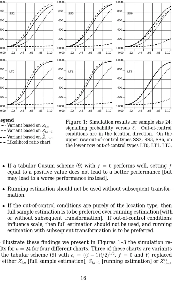
0.00 .22 .44 .66 .88 1.10 0.000 .200 .400 .600 .800 1.000 SS2 0.00 .22 .44 .66 .88 1.10 0.000 .200 .400 .600 .800 1.000 SS3 0.00 .22 .44 .66 .88 1.10 0.000 .200 .400 .600 .800 1.000 SS6 0.00 .22 .44 .66 .88 1.10 0.000 .200 .400 .600 .800 1.000 LT0 0.00 .22 .44 .66 .88 1.10 0.000 .200 .400 .600 .800 1.000 LT1 0.00 .22 .44 .66 .88 1.10 0.000 .200 .400 .600 .800 1.000 LT3 Legend Variant based onZ i;n Variant based onZ i;i 1 Variant based on ~ ~ Z i;i 1
Likelihood ratio chart
Figure 1: Simulation results for sample size 24: signalling probability versus Æ. Out-of-control conditions are in the location direction. On the upper row out-of-control types SS2, SS3, SS6, on the lower row out-of-control types LT0, LT1, LT3.
If a tabular Cusum scheme (9) with f = 0 performs well, setting f
equal to a positive value does not lead to a better performance [but may lead to a worse performance instead].
Running estimation should not be used without subsequent
transfor-mation.
If the out-of-control conditions are purely of the location type, then
full sample estimation is to be preferred over running estimation [with or without subsequent transformation]. If out-of-control conditions influence scale, then full estimation should not be used, and running estimation with subsequent transformation is to be preferred.
To illustrate these findings we present in Figures 1–3 the simulation re-sults forn =24for four different charts. Three of these charts are variants
of the tabular scheme (9) with c i = ((i 1)i=2) 1=2 , f = 0 and Y i replaced by either Z
i;n [full sample estimation], Z
i;i 1 [running estimation] or Z
i;i 1
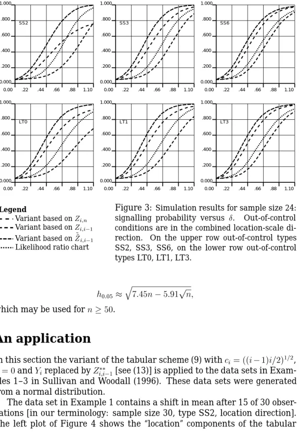
0.00 .22 .44 .66 .88 1.10 0.000 .200 .400 .600 .800 1.000 SS2 0.00 .22 .44 .66 .88 1.10 0.000 .200 .400 .600 .800 1.000 SS3 0.00 .22 .44 .66 .88 1.10 0.000 .200 .400 .600 .800 1.000 SS6 0.00 .22 .44 .66 .88 1.10 0.000 .200 .400 .600 .800 1.000 LT0 0.00 .22 .44 .66 .88 1.10 0.000 .200 .400 .600 .800 1.000 LT1 0.00 .22 .44 .66 .88 1.10 0.000 .200 .400 .600 .800 1.000 LT3 Legend Variant based onZ i;n Variant based onZ i;i 1 Variant based on ~ ~ Z i;i 1
Likelihood ratio chart
Figure 2: Simulation results for sample size 24: signalling probability versus Æ. Out-of-control conditions are in the scale direction. On the up-per row out-of-control types SS2, SS3, SS6, on the lower row out-of-control types LT0, LT1, LT3.
[running estimation with subsequent transformation]. The fourth chart is the likelihood ratio chart of Sullivan and Woodall (1996).
In particular, the simulation results suggest that the third variant con-sidered in Figures 1–3 [the tabular scheme (9) withc
i =((i 1)i=2) 1=2 ,f =0 andY i replaced by Z i;i 1
] is highly effective in detecting out-of-control con-ditions which may affect location as well as scale. In the remainder of this section we investigate the behavior of this tabular scheme under in-control conditions.
For n sufficiently large, theoretical considerations based on formula
(11.12) in Billingsley (1968) yield that h 0:001, h 0:005, h 0:01 and h 0:05 may be approximated by p 14:71n, p 11:70n, p 10:41nand p 7:45n, respectively. Plots
of the values in Table 1 versusnsuggest the following refinements:
h 0:001 q 14:71n+26:07 p n; h 0:005 q 11:70n+7:28 p n ; h 0:01 q 10:41n+1:61 p n;
0.00 .22 .44 .66 .88 1.10 0.000 .200 .400 .600 .800 1.000 SS2 0.00 .22 .44 .66 .88 1.10 0.000 .200 .400 .600 .800 1.000 SS3 0.00 .22 .44 .66 .88 1.10 0.000 .200 .400 .600 .800 1.000 SS6 0.00 .22 .44 .66 .88 1.10 0.000 .200 .400 .600 .800 1.000 LT0 0.00 .22 .44 .66 .88 1.10 0.000 .200 .400 .600 .800 1.000 LT1 0.00 .22 .44 .66 .88 1.10 0.000 .200 .400 .600 .800 1.000 LT3 Legend Variant based onZ i;n Variant based onZ i;i 1 Variant based on ~ ~ Z i;i 1
Likelihood ratio chart
Figure 3: Simulation results for sample size 24: signalling probability versus Æ. Out-of-control conditions are in the combined location-scale di-rection. On the upper row out-of-control types SS2, SS3, SS6, on the lower row out-of-control types LT0, LT1, LT3. h 0:05 q 7:45n 5:91 p n;
which may be used forn50.
An application
In this section the variant of the tabular scheme (9) withc i =((i 1)i=2) 1=2 , f =0andY ireplaced by Z
i;i 1 [see (13)] is applied to the data sets in
Exam-ples 1–3 in Sullivan and Woodall (1996). These data sets were generated from a normal distribution.
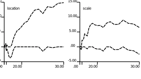
The data set in Example 1 contains a shift in mean after 15 of 30 obser-vations [in our terminology: sample size 30, type SS2, location direction]. The left plot of Figure 4 shows the “location” components of the tabular
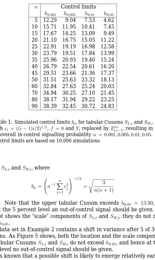
n Control limits h 0:001 h 0:005 h 0:01 h 0:05 5 12.29 9.04 7.53 4.62 10 15.71 11.95 10.41 7.45 15 17.67 14.25 13.09 9.49 20 21.10 16.75 15.05 11.22 25 22.91 19.19 16.98 12.58 30 23.79 19.51 17.84 13.99 35 25.96 20.93 19.40 15.24 40 26.79 22.54 20.61 16.20 45 29.51 23.66 21.36 17.37 50 31.51 25.63 23.32 18.13 60 32.84 27.63 25.24 20.03 70 34.94 30.25 27.10 21.45 80 38.17 31.94 29.22 23.25 90 38.39 32.45 30.72 24.83
Table 1:Simulated control limitsh
for tabular Cusums S L;iand S H ;i withc i = ((i 1)i=2) 1=2 ,f = 0 and Y i replaced by Z i;i 1 , resulting in an overall in-control signalling probability = 0:001;0:005;0:01 ;0 :05. Control limits are based on 10,000 simulations.
CusumsS L;iand S H ;i, where b n = 0 @ n 1 n X j=1 c 2 j 1 A 1=2 = s 3 n(n+1)
[cf. (8)]. Note that the upper tabular Cusum exceeds h 0:05
= 13:99, and
hence at the 5 percent level an out-of-control signal should be given. The right plot shows the “scale” components ofS
L;i and S
H ;i; they do not move
beyondh 0:05.
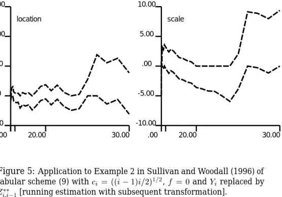
The data set in Example 2 contains a shift in variance after 5 of 30 ob-servations. As Figure 5 shows, both the location and the scale components of the tabular Cusums S
L;i and S
H ;ido not exceed h
0:05, and hence at the 5
percent level no out-of-control signal should be given.
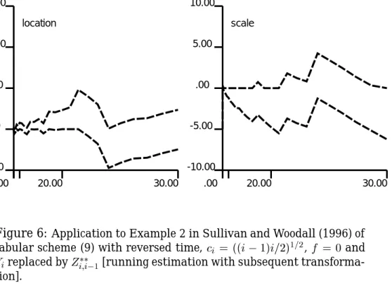
If it is known that a possible shift is likely to emerge relatively early in the sample, then one may reverse time in order to profit of the sensitivity of the tabular Cusums to shifts occurring relatively late in the sample. As Figure 6 shows, reversing time also does not lead to an out-of-control signal at the 5 percent level.
location .00 20.00 30.00 -5.00 .00 5.00 10.00 15.00 scale .00 20.00 30.00 -5.00 .00 5.00 10.00 15.00
Figure 4: Application to Example 1 in Sullivan and Woodall (1996) of tabular scheme (9) withc
i = ((i 1)i=2) 1=2 ,f = 0 and Y i replaced by Z i;i 1
[running estimation with subsequent transformation].
In contrast, the likelihood ratio test chart does give an out-of-control sig-nal. This is contrary to what is expected: in our terminology we are dealing here with the SS6 type in reversed time, and our simulations show that in this case the likelihood ratio test chart is inferior to the chart depicted in Figure 6 [cf. the upper-right plot of Figure 2].
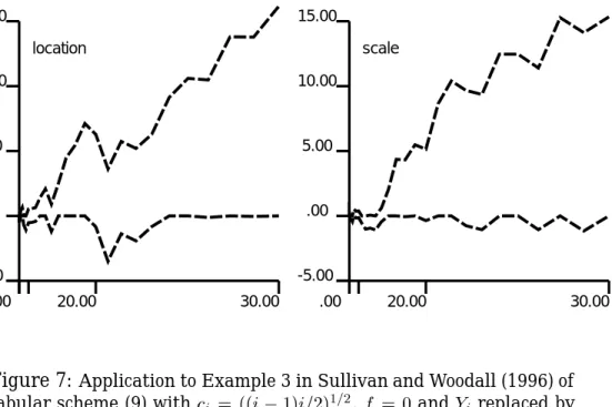
Finally, the data set in Example 3 exhibits a shift in both mean and variance after 15 of 30 observations. Figure 7 shows that both the loca-tion and the scale component of the upper tabular Cusum exceedh
0:05, and
hence at the 5 percent level an out-of-control signal should be given.
References
[1] Box, G., Ramirez, J. (1992). “Cumulative score charts”. Quality and
Reliability Engineering International 8, 17–27.
[2] Brown, R.L., Durbin, J., Evans, J.M. (1975). “Techniques for testing the constancy of regression relationships over time”. Journal of the
Royal Statistical Society B37, 149-163.
[3] Del Castillo, E., Montgomery, D.C. (1994). “Short-run statistical pro-cess control: Q-chart enhancements and alternative methods”. Qual-ity and ReliabilQual-ity Engineering International 10, 87–97.
location .00 20.00 30.00 -5.00 .00 5.00 10.00 15.00 scale .00 20.00 30.00 -10.00 -5.00 .00 5.00 10.00
Figure 5: Application to Example 2 in Sullivan and Woodall (1996) of tabular scheme (9) withc
i = ((i 1)i=2) 1=2 ,f = 0 and Y i replaced by Z i;i 1
[running estimation with subsequent transformation].
[4] H ´ajek, J., ˇSid ´ak, Z. (1967). Theory of rank tests. Academic Press, New York.
[5] Hawkins, D.M. (1991). “Diagnostics for use with regression recursive residuals”. Technometrics 33, 221–234.
[6] Hawkins, D.M., Olwell, D.H. (1998). Cumulative sum charts and
charting for quality improvement. Springer-Verlag, New York.
[7] Hinkley, D.V. (1971). “Inference about the change-point from cumula-tive sum tests”. Biometrika 58, 509–523.
[8] Kallenberg, W.C.M., Koning, A.J. (1995). “On Wieand’s theorem”.
Statistics & Probability Letters 25, 121–132.
[9] Koning, A.J. (1999). “A general Cusum chart for preliminary analysis of individual observations”. Bulletin of the International Statistical
In-stitute.
[10] Koning, A.J. and Does, R.J.M.M. (1999). “Cusum charts for prelimi-nary analysis of individual observations”. Journal of Quality
location .00 20.00 30.00 -5.00 .00 5.00 10.00 15.00 scale .00 20.00 30.00 -10.00 -5.00 .00 5.00 10.00
Figure 6: Application to Example 2 in Sullivan and Woodall (1996) of tabular scheme (9) with reversed time, c
i =((i 1)i=2) 1=2 ,f = 0 and Y ireplaced by Z i;i 1
[running estimation with subsequent transforma-tion].
[11] Lehmann, E.L. (1994). Testing Statistical Hypotheses. Second edition. Chapman and Hall, London.
[12] Lindsey, J.K. (1996). Parametric Statistical Inference. Oxford Univer-sity Press.
[13] Lucas (1982). “Combined Shewhart-CUSUM quality control schemes”.
Journal of Quality Technology 14, 51–59.
[14] Montgomery, D.C. (1996). Introduction to Statistical Quality Control,
third edition. Wiley, New York.
[15] Quandt, R.E. (1960). “Tests of the hypothesis that a linear regression system obeys two seperate regimes”. Journal of the American
Statis-tical Association 55, 324–330.
[16] Quesenberry, C.P. (1991). “SPC Q charts for start-up processes and
short or long runs”. Journal of Quality Technology 23, 213–224.
[17] Quesenberry, C.P. (1995). “On properties of Q charts for variables”.
location .00 20.00 30.00 -5.00 .00 5.00 10.00 15.00 scale .00 20.00 30.00 -5.00 .00 5.00 10.00 15.00
Figure 7: Application to Example 3 in Sullivan and Woodall (1996) of tabular scheme (9) withc
i = ((i 1)i=2) 1=2 ,f = 0 and Y i replaced by Z i;i 1
[running estimation with subsequent transformation].
[18] Sullivan, J.H., Woodall, W.H. (1996). “A control chart for preliminary analysis of individual observations”. Journal of Quality Technology 28, 265–278.
[19] Worsley, K.J. (1986). “Confidence regions and tests for a change-point in a sequence of exponential family random variables”. Biometrika 73, 91–104.