Australian Asian Options
Manuel Moreno Javier F. Navas
Department of Economics and Business Department of Finance Universitat Pompeu Fabra Instituto de Empresa Carrer Ramon Trias Fargas, 25-27 Mar´ıa de Molina, 13 08005 Barcelona, Spain 28006 Madrid, Spain phone: +34 935422771 phone: +34 915689600 fax: +34 935421746 fax: +34 915636859 e-mail: [email protected] e-mail: [email protected]
This Version: February 25, 2003
Acknowledgments
We would like to thank Arturo Kohatsu and seminar participants at the Universidad Pablo de Olavide, Universitat Pompeu Fabra and Universidad de Navarra for their valuable suggestions and comments. The first author gratefully acknowledgesfinancial support by DGESIC grant BEC2002-00429. The second author thanks the hospitality of the Universitat Pompeu Fabra, where part of this work was done. The usual caveat applies.
Australian Asian Options
Abstract
We study European options on the ratio of the stock price to its average and viceversa. Some of these options are traded in the Australian Stock Exchange since 1992, thus we call them Australian Asian options. For geometric av-erages, we obtain closed-form expressions for option prices. For arithmetic means, we use different approximations that produce very similar results.
Keywords: Asian Options, Arithmetic Average, Geometric Average, Edge-worth Expansion, Lognormal Distribution, Gamma Distribution.
1
Introduction
Asian options are options on average values of asset prices. Their prices depend on the asset price history over the averaging period. Therefore, they are considered path-dependent claims.
These derivatives are traded in over-the-counter markets1and it is usually argued that they provide the following advantages: (a) they are cheaper than standard European ones as the average is less volatile than the asset price itself, (b) this type of options prevents manipulation of the underlying asset price at the maturity date and (c) they are the adequate hedging instrument for traders who act continuously over finite periods.
Options on the ratio of the stock price to its average (or viceversa) are particular cases of Asian options. They have recently appeared as special types of variable purchase options (VPOs). VPOs were first issued in 1992 and have been traded since then on the Australian Stock Exchange. A VPO is an option that gives its holder the right to buy at maturity a stochastic number of shares that depends on the terminal stock price. This option can have more complex features like caps and floors on the number of shares. Handley (2000) provides a detailed description of VPOs as well as pricing formulae. He also describes Asian VPOs, in which the number of shares that can be bought at maturity depends on the average stock price. These options are shown to be equivalent to options on the ratio of the stock price to its average. Alternatively, we could define Asian VPOs in such a way that they are equivalent to options on the ratio of the average of the stock price to the stock price itself.
(discrete- and continuous-time) means of stock prices that are assumed to follow a lognormal process.2 When the average is computed on geometric basis, these ratios are lognormally distributed at maturity, thus we obtain Black-Scholes-type formulae to price options.
However, when the average is computed on arithmetic basis, the risk-neutral distribution of these ratios is, in general, unknown and we can not obtain closed-form expressions for the prices of these options.3 This happens
because the arithmetic average is the convolution of correlated lognormal random variables and its distribution is unknown.4
Some of the approaches that have been followed in the literature to study the pricing and hedging of arithmetic Asian options are:
• Numerical approximations
— Finite different schemes. In this case, a partial difference pric-ing equation is obtained and then solved numerically. See, for instance, Kemna and Vorst (1990), Rogers and Shi (1995), Alziari et al(1997) or Hansen and Jorgensen (2000).5
— Monte Carlo simulations. Here, variance reductions technique are commonly used to reduce standard errors. For example, Kemna and Vorst (1990) use the closed-form expressions for prices of geo-metric Asian options as control variables to price arithmetic ones with Monte Carlo.6
• General numerical methods. Some examples are the fast Fourier trans-form proposed in Carverhill and Clewlow (1990), the conditioning ap-proach suggested in Curran (1994), Rogers and Shi (1995) and Nielsen
and Sandmann (1996, 1999, 2001), and the accelerated simulation method presented in V´azquez-Abad and Dufresne (1998).
• Pseudo-analytic characterizations. this is the case of Yor (1992, 1993), Geman and Yor (1993), De Schepper et al (1994), Eydeland and Ge-man (1995), Fu et al(1999) and Shirakawa (1999), who use the theory of Bessel processes and the inversion of a Laplace transform. Alterna-tively, Ju (1997) employs A Fourier transform, while Dufresne (2000) suggests a Laguerre expansion.
• Analytical approximations. Jarrow and Rudd (1982) apply Edgeworth series expansion to the problem of option pricing when the risk-neutral distribution of the underlying asset at maturity is not known. Typ-ically, up to fourth order moments are used to approximate the true probability density function. This method has been also used by Turn-bull and Wakeman (1991), Ritchken et al (1993) and Jacques (1996). Some authors use only the first and second order moments in the Edgeworth series expansion, obtaining what is called the Wilkinson approximation.7 This is equivalent to assume that the true
distribu-tion is actually lognormal, so that Black-Scholes-type formulae can be used to price options. See Levy and Turnbull (1992) for a numerical comparison of the accuracy of these expansions. Other analytical ap-proximations can be seen in Bouaziz et al (1994), Vorst (1990, 1992, 1996), Nielsen and Sandmann (1998), Posner and Milevsky (1998) and Chung et al (2001).
and Posner (1998) who use the fact that the infinite sum of correlated lognormal random variables is reciprocal gamma distributed to obtain a closed-form solution for the value of arithmetic Asian options.8 This
formula is exact only when the average is computed continuously.
In this paper we price arithmetic Australian Asian options using both the Wilkinson approximation and the gamma distribution. We also use Monte Carlo simulation with antithetic variables. The results show that option prices obtained with the three methods are quite similar. This is true even when the number of monitoring dates used to compute the average is small. Hence, in practice, it does not seem to be necessary to use higher order moments in the Edgeworth expansion nor to require a large number of mon-itoring dates in the gamma approximation to the option pricing problem.
The rest of the paper is organized as follows. Section 2 describes some statistical results that are used in the paper. In Section 3 we generalize the Black-Scholes formula for option prices. Section 4 presents closed-form expressions for the prices of geometric Australian Asian options and Section 5 presents approximations to the value of arithmetic ones. Finally, Section 6 summarizes and concludes.
2
Previous Statistical Results
The following Lemma specifies several features of the lognormal distribution that will be useful to find later results:
Lemma 1
1. Let Y = ln(X)be a normal random variable with mean mand variance s2. Then, X follows a lognormal distribution, that is, X
∼ Λ(m, s2).
Its density function is given by f(x) = 1 sx√2π exp − 1 2 Ã lnx−m s !2 , x >0 (1)
Moreover, it is verified that
E(X) = exp ½ m+1 2s 2¾ (2) V(X) = [E(X)]2hes2 −1i (3) E(X−1) = exp{−2m}E(X) (4) V(X−1) = [E(X−1)]2hes2 −1i (5) 2. The expectation of the truncated lognormal variable
˜ X = X if X ≥K 0 if X < K , K ∈IR+ is given by E( ˜X) =E(X)N(s−D), D= lnK −m s
where N(.) denotes the distribution function of a standard normal vari-able.
Proof: See Appendix.
The following Lemma will be useful to compute the moments of ratios involving arithmetic average asset prices:
Lemma 2 (Mood et al (1974))
Let X and Y be two random variables. Then, it is verified that E
µX Y
' E(X)E(Y) − (E(Y1 ))2Cov(X, Y) +
E(X) (E(Y))3V(Y) V µX Y ¶ ' Ã E(X) E(Y) !2Ã V(X) (E(X))2 + V(Y) (E(Y))2 −2 Cov(X, Y) E(X)E(Y) !
Proof: See Moodet al, p. 181.
3
The Generalized Black-Scholes Model
Uncertainty is modelled by a filtered probability space (Ω,IF, P). The set of trading dates is t∈[0, T]. Let Z ={Zt|t ∈[0, T]} be the price process for
the underlying asset. The assumptions of the pricing model are as follows: 1. Markets are frictionless
(a) No transaction costs when trading the stock or the option (b) No taxes
(c) No penalties to short selling (d) All assets are perfectly divisible 2. Security trading is in continuous time
3. The term structure of interest rates is flat and known with certainty. Let β = { βt; t ∈ [0, T] } be the value process for a banking account
defined by
dβt=rβtdt, (6)
4. The asset offers a continuous dividend yield of δ in the interval [0, T] 5. The asset price follows a GBM process
dZt=µZZtdt+σZZtdWt, (7)
where (Zt, t) ∈ (0,∞)×[0, T], µZ and σZ are constants and Wt is a
standard Wiener process. Usually, σZ2 is referred to as the logarithmic
variance parameter of the asset.
Under the risk-neutral probability measure, the process (7) becomes dZt =αZZtdt+σZZtdWt
where αZ is the (constant) risk-neutral drift of the process.
The solution for this process is given by
Zt=Z0exp ½µ αZ− 1 2σ 2 Z ¶ t+σZWt ¾
Therefore,Ztfollows a lognormal process. Moreover, it is straightforward to
show that [lnZu]|Zt ∼N µ ln(Zt) + µ αZ− 1 2σ 2 Z ¶ (u−t),σZ2(u−t) ¶ , u > t (8)
Lemma 3 The moments of the variable Zt under the risk-neutral measure
are the following:
E(Zt) = Z0eαZt V(Zt) = [E(Zt)]2 h eσ2Zt−1 i Cov(Zt, Zs) = Z02eαZ(t+s) h eσZ2s−1 i , s < t
Proof: See Appendix.
Obviously, for s=t, we obtain Cov(Zt, Zt) =Z02eαZ(t+t) h eσ2Zt−1 i =Z02e2αZt h eσ2Zt−1 i =V(Zt)
The following proposition generalizes the Black-Scholes option pricing formula:
Proposition 1 The price at time 0 of an European call option on Z that matures at time T and with strike price K is given by
C(Z,0, T, K) =e−rTE(ZT)N(d1)−Ke−rTN(d2) (9) where d1 = ln³e−αZTE(ZT)/K ´ +³αZ+12σZ2 ´ T σZ √ T d2 = d1−σZ √ T
Proof: See Appendix.
The prices of European put options can be easily obtained using the put-call parity:
P(Z,0, T, K) =C(Z,0, T, K)−e−rTE(ZT) +Ke−rT (10)
Let St denote the stock price at time t. We suppose that St follows the
risk-neutral process
where q is the continuous dividend yield of the stock and σ is a constant. The solution for this process is given by
St=S0exp ½µ r−q−1 2σ 2¶ t+σWt ¾ (12) Note that application of Proposition 1 to the stock price process (11) leads to the Black-Scholes formula adjusted by dividends, as derived by Merton (1973).
4
Geometric Australian Asian Options
We consider nmonitoring dates so that the time interval [0, T] is partitioned in the following way:
{t0 = 0< t1 < t2 <· · ·< tn=T}, ti−ti−1 =
T
n =∆t, ∀i= 1,· · ·, n. Let S = { Sti ≡ Si, i = 0,1,· · ·, n } be the price process for the stock. We define the geometric mean of the nstock prices S1,· · ·, Sn as
Gn= (S1· · ·Sn) 1 n = Ã n Y i=1 Si !1 n , G0 ≡S0 Using (12), we have Gn=S0exp (µ r−q− 1 2σ 2¶n+ 1 2 ∆t+ σ n n X i=1 Wti ) (13)
Looking at (12) and (13), and usingtn =n∆t, we have
Sn Gn = exp (µ r−q− 1 2σ 2 ¶n −1 2 ∆t+ σ n " n Wtn− n X i=1 Wti #) (14) Gn Sn = exp ( − µ r−q−1 2σ 2¶n−1 2 ∆t− σ n " n Wtn− n X i=1 Wti #) (15)
It is clear from (13)-(15) that the geometric average and both ratios are lognormally distributed. Consequently, we can apply Proposition 2 to price options on these assets after computing their moments. We now state a Lemma that will be useful to obtain these prices.
Lemma 4 Given the Brownian motions Wti, i= 1,· · ·, n, it is verified that
V Ã n X i=1 Wti ! = (n+ 1) ³ n+ 12´n 3 ∆t V Ã n Wtn− n X i=1 Wti ! = (n−1) ³ n− 12´n 3 ∆t
Proof: See Appendix.
Proposition 2 We consider European call options on Sn/Gn and Gn/Sn
that mature at time T and with strike price K. The prices at time 0 of these options are given by expression (9), where the expected value and the logarithmic variance of the asset at maturity are given by the following table:9
Zn E(Zn) σZ2T Gn S0exp n³ r−q− n6−n1σ2´n2+1n To (n+1)(n+ 1 2) 3n2 σ 2T Sn/Gn exp n³ r−q− n6+1n σ2´n−1 2n T o (n−1)(n−1 2) 3n2 σ2T Gn/Sn exp n −³r−q−5n6−n1σ2´n−1 2n T o (n−1)(n−1 2) 3n2 σ2T
Proof: See Appendix.
The expression obtained in this Proposition is the Black-Scholes formula with a volatility parameter σZ and a continuous dividend yield δ=r−αZn as given by the next table:
Zn δ Gn ³ n−1 n+1r+q+ n−1 6n σ 2´n+1 2n Sn/Gn ³ n+1 n−1r+q+ n+1 6n σ 2´n−1 2n Gn/Sn ³ 3n−1 n−1r−q− 5n−1 6n σ 2´n−1 2n
Note that the prices of Australian Asian options do not depend on the current stock price, S0.
Obviously, when Zn = Sn, we obtain the Black-Scholes formula which
does not depend on the partition of the time interval. When Zn = Gn, we
get the price derived by Turnbull and Wakeman (1991) and Ritchken et al (1993).
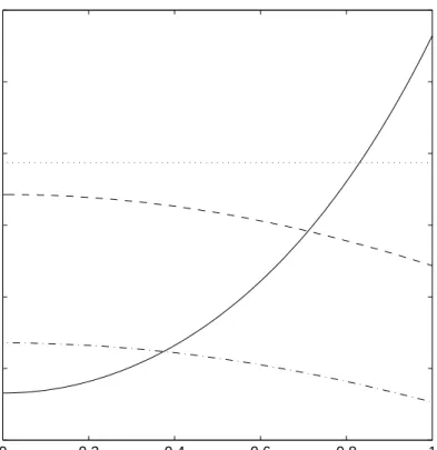
The effect of the number of monitoring dates (n) on the expected value of the asset is not clear, since it depends on the relationship among r, q and σ. However, the effect of n on the logarithmic variance, σ2
ZT, is quite obvious
as can be seen in Figure 1. The parameter values are σ = 0.2 and T = 1. [ Insert Figure 1 about here ]
We observe the following facts:
• The logarithmic variance of the stock price is constant.
• The logarithmic variance ofGn is equal to that of the stock price when
n= 1. Then it decreases withn, and converges to σ32T, the logarithmic variance of the continuous geometric average, obtained by Kemna and Vorst (1990).
• The logarithmic variances of Sn/Gn and Gn/Sn are equal. This is due
its reciprocal (see expressions (3)-(5)). This variance increases with n and converges to σ32T.
It can also be of interest to study the effect of σ and T on option prices. We leave this analysis for the case of continuous-time means.
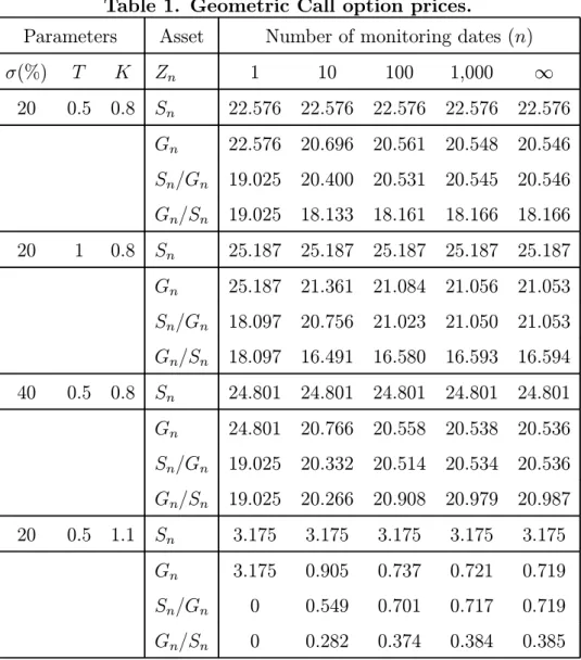
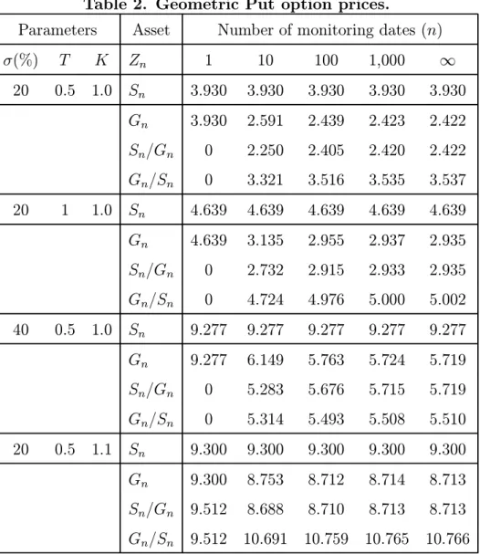
Tables 1 and 2 show call and put option prices respectively (multiplied by 100) for different cases and monitoring dates. Call prices are computed using Proposition 2. Put prices are obtained applying expression (10). The interest rate is 10 % and the stock dividend yield is 3 %. We include the stock price (Sn) and its geometric average (Gn) as underlying assets as a
reference. In both cases, we assume that the initial stock price (S0) is 1.
[ Insert Tables 1 and 2 about here ]
We see that the value of the Australian Asian options are relatively similar to those of geometric Asian options.
For one monitoring dateandGn =ST, we see that options onGnhave the
same value as those on the stock. Moreover, Australian options are equal to options on the unity, and their values are given by exp{−rT}max{1−K,0}. Interestingly, option prices do not necessarily increase with the volatility of the stock price (σ) either. This is also true for standard geometric Asian options. For example, from Table 1 we have that when T = 0.5, K = 0.8, and n = 1,000 the call option on Gn has a value of 20.548 and 20.538 for
σ = 0.2 and 0.4, respectively.10
We see that option prices do not necessarily increase with time to maturity (T). For example, when σ = 0.2, K = 0.8, and n= 100, Table 1 shows that
the call option on Gn/Sn has a value of 18.161 and 16.580 for maturities of
0.5 and 1.0 years, respectively.
The tables show that option prices do not change monotonically with n. For instance, in Table 1 we have that when σ = 0.2, T = 0.5, and K = 1.1, call options prices on Gn are 3.175, 0.905, and 0.737, when n = 1,10 and
100, respectively.
The effect of a change in the exercise price (K) is as expected: call prices decrease and put prices increase with K.
As additional reference, the Black-Scholes call option prices (dividend yield = 0) in the four cases studied in Table 1 are 24.027, 27.993, 26.081, and 3.743, and the Black-Scholes put option prices corresponding to Table 2 are 3.400, 3.753, 8.703, and 8.378, respectively.
We now define the continuous geometric average of the stock price over the interval [0, T] as GT = exp ( 1 T Z T 0 ln(St)dt ) Using (12), we have GT =S0exp ( 1 2 µ r−q− 1 2σ 2¶T + σ T Z T 0 Wtdt ) (16) Looking at (12) and (16), we have
ST GT = exp ( 1 2 µ r−q− 1 2σ 2 ¶ T + σ T " T WT − Z T 0 Wtdt #) (17) GT ST = exp ( −12 µ r−q− 1 2σ 2 ¶ T − σ T " T WT − Z T 0 Wtdt #) (18) We now state a Lemma that will be useful to compute the prices of options on these assets.
Lemma 5 Given the Brownian motions Wt, t∈[0, T], it is verified that V ÃZ T 0 Wtdt ! =V Ã T WT − Z T 0 Wtdt ! = T 3 3
Proof: See Appendix.
Proposition 3 We consider European call options on ST/GT and GT/ST
that mature at time T and with strike price K. The prices at time 0 of these options are given by expression (9), where the expected value and the logarithmic variance of the asset at maturity are given by the following table:11
ZT E(ZT) σ2ZT ST S0exp{(r−q)T} σ2T GT S0exp n 1 2 ³ r−q− 16σ2´To σ2 3T ST/GT exp n 1 2 ³ r−q− 16σ2´To σ32T GT/ST exp n −12 ³ r−q− 56σ2´To σ2 3T Proof: See Appendix.
The option pricing formula given in this Proposition corresponds to a continuous dividend yield δ =r−αZT as given by the next table:
ZT δ ST q GT, ST/GT 12 ³ r+q+16σ2´ GT/ST 12 ³ 3r−q− 56σ2´ Notice that:
• The logarithmic variances of both ratios are equal to the one derived by Kemna and Vorst (1990) for the continuous geometric average. The in-tuition for this result is that, with infinite monitoring dates, the volatil-ity of the ratio depends only on the volatilvolatil-ity of the average. This value
increases with σ and is one third of the variance in the Black-Scholes formula.
• The expected value of GT is S0 times the expected value of ST/GT. • The expected values ofST/GT andGT/ST do not depend on the current
stock price, S0.
• The expected values of GT and ST/GT are smaller than that of ST.
Figure 2 shows E(ZT) as a function of σ. The parameter values are
r = 10%, q= 3%, T = 1. We assume S0 = 1.2.
[ Insert Figure 2 about here ]
We observe that the expected values ofGT and ST/GT decrease with σ,
while the expected value of GT/ST increases withσ.12
Since the logarithmic variance of the assets studied increase withσ, and their expected values also depend on σ, we have that option prices can de-crease with volatility or time to maturity. This surprising result is analyzed next with more detail.
a) Theta
To study the effect of a change in T on option prices, we compute the corresponding partial derivative. Replacing the expected value and the loga-rithmic variance of the asset at maturity in (9) as given in Proposition 1 and differentiating with respect to T, we get
∂C(.) ∂T =e −rT " (αZT −r)E(ZT)N(d1) +KrN(d2) + σZ 2√TE(ZT)N 0(d 1) # (19)
If q > 0, we have that αZT −r < 0 for all the assets except for GT/ST. Consequently, the effect ofT on call options on these assets is undetermined. Ifq = 0, we have thatαsT −r= 0, and the stock call price increases with T. For the ratio GT/ST, we have that αZT −r >0 ⇔r <
1 3
³
q+56σ2´. In this case, an increase in T leads to a higher call option price.
To analyze the effect of an increase of T on the put price, we use the put-call parity (10) and the derivative obtained in (19) to get
∂P(.) ∂T =e −rT " (r−αZT)E(ZT)N(−d1)−KrN(−d2) + σZ 2√TE(ZT)N 0(d 1) # (20) The sign of this derivative can be positive or negative, depending on the parameter values. For all the assets except GT/ST, we have r−αZT ≥ 0. Then, for these assets, the effect of T on the put price depends on how large is the second term into brackets. If the exercise price is low enough, the put price will increase withT, while for large strikes the opposite will take place. For the ratio GT/ST, we have that r−αZT >0 ⇔r >
1 3
³
q+56σ2´. In this
case, an increase in T can lead to a higher put price if the exercise price is small.
Figure 3 plots geometric Australian option prices as a function of time to maturity. The averages are computed with infinite monitoring dates. The parameters are: r = 0.1, q = 0.03, σ = 0.2, K = 0.8 for calls and K = 1.2 for puts.
[ Insert Figure 3 about here ]
We see that, in this case, the price of a call option on ST/GT increases
latter result is due to the fact that r > 13³q+56σ2´, so thatα
ZT−r <0 and
∂C(.)/∂T can be negative.
Since the exercise price for the put options is relatively high (K = 1.2), we see that the price of the put option onST/GT decreases withT. The same
occurs for a put option on GT/ST when time to maturity is small (between
0 and 0.65 years). For higher T, the put price increases. When T > 1.5, the put price decreases again. Interestingly, if we reduce the exercise price to K = 1.1, the put price increases for all T.
b) Vega
Replacing the expected value and the logarithmic variance of the asset at maturity in (9) as given in Proposition 1 and differentiating the resulting expression with respect to σ, we obtain that the effect of a change in σ on the price of a call option is given by
νC = ∂C(.) ∂σ =e −rTE(Z T) √ T " ∂αZ ∂σ √ T N(d1) + ∂σZ ∂σ N 0(d 1) # (21)
The partial derivatives into brackets are: ZT ∂αZ∂σ ∂σZ∂σ ST 0 1 GT −16σ √13 ST/GT −16σ √13 GT/ST 56σ √13 Therefore, we obtain νC(ST) = ∂C(.) ∂σ =S0 √ T N0(d1)>0
νC(GT) = ∂C(.) ∂σ =e −rTE(G T) √ T " −16σ√T N(d1) + 1 √ 3N 0(d 1) # νC(ST/GT) = ∂C(.) ∂σ =e −rTE(S T/GT) √ T " −16σ√T N(d1) + 1 √ 3N 0(d 1) # νC(GT/ST) = ∂C(.) ∂σ =e −rTE(G T/ST) √ T " 5 6σ √ T N(d1) + 1 √ 3N 0(d 1) # >0 It is straightforward to show that
νC(GT)<0⇔ N0(d 1) σN(d1) < 1 2 s T 3 νC(ST/GT)<0⇔ N0(d 1) σN(d1) < 1 2 s T 3
Hence, the vega of a call option on in the Kemna and Vorst (1990) model and the vega of a geometric Australian asian call option on ST/GT can be
negative. As shown later, this can occur for reasonable parameter values. To analyze the effect of an increase of σ on the put price, we use the put-call parity (10) and the derivative obtained in (21) to obtain
νP = ∂P(.) ∂σ =e −rTE(Z T) √ T " ∂σZ ∂σ N 0(d 1)− ∂αZ ∂σ √ T N(−d1) # (22) Therefore, the vega of put options on our assets are:
νP(ST) = ∂P(.) ∂σ =S0 √ T N0(d1)>0 νP(GT) = ∂P(.) ∂σ =e −rTE(G T) √ T " 1 6σ √ T N(−d1) + 1 √ 3N 0(d 1) # >0 νP(ST/GT) = ∂P(.) ∂σ =e −rT E(ST/GT) √ T " 1 6σ √ T N(−d1) + 1 √ 3N 0(d 1) # >0 νP(GT/ST) = ∂P(.) ∂σ =e −rTE(G T/ST) √ T " −5 6σ √ T N(−d1) + 1 √ 3N 0(d 1) # It is clear that νP(GT/ST)<0⇔ N0(d1) σN(−d1) < 5 2 s T 3
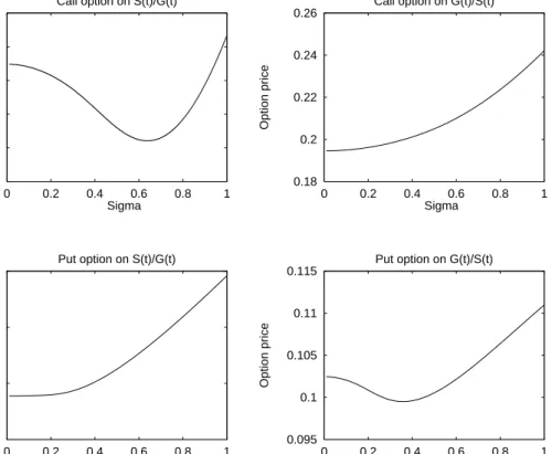
As before, this inequality can hold for reasonable parameter values. Figure 4 exhibits geometric Australian option prices as a function of volatility (σ). The averages are computed with infinite monitoring dates. The parameters are: r = 0.1, q = 0.03, T = 0.1, K = 0.8 for calls and K = 1.1 for puts.
[ Insert Figure 4 about here ]
We see that the price of the call option onST/GT first decreases and then
increases with volatility. The vega of this option is zero when σ = 0.67. As expected, the price of the call option on GT/ST and a put option onST/GT
always increase with σ. However, the price of the put option onGT/ST first
decreases and then increases with volatility. The vega of this option is zero when sigma= 0.36.
To summarize the results, both call and put geometric Australian option prices can increase and decrease with either time to maturity or volatility. This is clearly seen in Figure 5, that shows option prices as a function of both variables. The parameter values are: r = 0.1, q= 0.03, n=∞, K = 0.8 for the call option and K = 1.1 for the put option.
[ Insert Figure 5 about here ]
Finally, Tables 1 and 2 present geometric option prices whenn=∞. Note that the option on Sn/Gn is equivalent to the option on Gn. This happens
because we are taking S0 = 1. We see that option prices for continuous
aver-ages are almost identical to those for discrete averaver-ages with 1,000 monitoring dates. For example, from Table 2 we have that whenσ = 0.2, T = 1, K = 1.0
and n=∞, the put options on Gn, Sn/Gn, and Gn/Sn have values of 2.935,
2.935, and 5.002, respectively, while that when n = 1,000 those prices are 2.937, 2.933, and 5.000, respectively.
5
Arithmetic Australian Asian Options
We define the discrete arithmetic mean of the nstock prices S1,· · ·, Sn as
An = 1 n(S1+· · ·+Sn) = 1 n n X i=1 Si, A0 ≡S0 (23)
The continuous counterpart is given by
AT =
1 T
Z T
0 Stdt (24)
As mentioned previously, the distribution of An is unknown. Therefore,
we can not apply Proposition 1 to price options. As described in the following sections, two ways to overcome this problem are:
• To approximate the true distribution with an alternative one.
• To approximate the distribution of An with that of AT.
5.1
Pricing the Options with the Edgeworth /
Wilkin-son Approximation
To price options, we approximate the risk-neutral distribution of the un-derlying asset at maturity with a tractable distribution. We perform this approximation by expanding the true distribution around the approximating one. This approach is called generalized Edgeworth series expansion. The
coefficients of this expansion are function of the moments of the true and approximating distribution. Considering up to four terms in this expansion and specifying the approximating distribution to be lognormal, we will show that the (approximate) option price is equal to the Black-Scholes price plus three adjustment terms. These terms depend, respectively, on the difference between the variance, skewness, and kurtosis of the true and the lognormal distribution. The intuition is that the first four moments of the distribution are enough to reflect the effects of the distribution on option prices.
More concretely, we approximate the true probability distribution, F(s), with an approximating distribution, A(s). It is assumed that both distri-butions have continuous density functions, f(s) and a(s). We employ the following notation: αj(F) = Z ∞ −∞s jf(s)ds µj(F) = Z ∞ −∞(s−α1(F)) j f(s)ds Ψ(F, t) = Z ∞ −∞e itsf(s)ds, i=√ −1
where αj(F) and µj(F) are, respectively, the j-th non-central and central
moments of F and Ψ(F, t) is the characteristic function of F.13
Following Stuart and Ord (1987), the cumulantskj(F) of the distribution
F are defined by the identity in t
exp X∞ j=1 kj(F) tj j! = ∞ X j=0 αj(F) tj j! or, equivalently lnΨ(F, t) = ∞ X j=1 kj(F) (it)j j!
For practical purposes, we only need thefirst four cumulants in the Edge-worth series expansion. These cumulants are, respectively, the mean, the variance, the coefficient of skewness and the excess of kurtosis:
k1(F) = α1(F), k2(F) =µ2(F)
k3(F) = µ3(F), k4(F) = µ4(F)−3µ22(F)
Jarrow and Rudd (1982) prove the following series expansion for f(s) around a(s): f(s) = a(s) + k2(F)−k2(A) 2! d2a(s) ds2 − k3(F)−k3(A) 3! d3a(s) ds3 +k4(F)−k4(A) + 3(k2(F)−k2(A)) 2 4! d4a(s) ds4 +ε(s) (25)
where, by construction, k1(F) is set equal tok1(A).
The difference between f(s) and a(s) depends on the cumulants of both distributions with weighting factors given by the derivatives of a(s). The terms on the right-hand side of (25) reflect any difference in variance, skew-ness and kurtosis and variance between f(s) and a(s). The residual error,
ε(s), includes any remaining difference.
Now, we employ (25) to obtain an approximate option price. Using f(s) as the true distribution of the asset price at maturity, we obtain the expected value at maturity of an option on this asset. Then, this expansion provides an approximated expected value for the option at maturity in terms of the approximating distribution, a(s).
In a risk-neutral world, the true price of the call option,C(F), is obtained by discounting its expected value at the risk-free rate:
C(F) =e−rT Z ∞
−∞
Using (25) and a little algebra, this price becomes C(F) = C(A) +e−rTk2(F)−k2(A) 2! a(K)−e −rTk3(F)−k3(A) 3! da dST ¯ ¯ ¯ ¯ ¯K +e−rTk4(F)−k4(A) + 3(k2(F)−k2(A)) 2 4! d2a dS2 T ¯ ¯ ¯ ¯ ¯ K +ε(K) (26) where C(A) =e−rT Z ∞ −∞max{ST −K,0}dA(ST)
A natural candidate for the approximating distribution is the lognormal one. In this case, C(A) is equal to the Black-Scholes option price.
Equation (26) shows that the true option price is equal toC(A) plus three adjustment terms. As before, these terms correct for difference in variance, skewness and kurtosis and variance between the distributionsF and Awhile the term ε(K) includes the residual error.
As mentioned in the Introduction, the Wilkinson approximation is a par-ticular case of the Edgeworth expansion, where just the first two cumulants are used.
5.2
Pricing the Options with the Gamma Distribution
It is known that the infinite sum of lognormal distributions is a reciprocal gamma distribution. Using this distribution as state-price density function, Milevsky and Posner (1998) obtain a closed-form expression for the price of arithmetic Asians options. The solution is the same as the Black-Scholes formula where the normal distribution is replaced by the gamma one.We briefly summarize the main characteristics of the gamma distribution. LetX be gamma distributed with parametersαand β, that is,X ∼Γ(α,β).
Its density function is given by g(x) = β −αxα−1expn −βx o Γ(α) , x >0 where Γ(x) is the gamma function, defined as
Γ(x) = Z ∞
0 t
x−1e−tdt
The mean and variance of the gamma distribution are E(X) =αβ, V(X) =αβ2.
If we defineY = X1, then Y follows a reciprocal gamma distribution. Its first two non-central moments are
M1 = E(Y) = 1 β(α−1) M2 = E(Y2) = 1 β2(α−1)(α−2)
The variance is given by
V(Y) =M2−M12 =
1
β2(α−1)2(α−2)
It is straightforward to obtain the following relationships:
α = 2M2−M 2 1 M2−M12 , β = M2−M 2 1 M1M2 (27) Hence, to price option, we must obtain thefirst two risk-neutral moments (M1, M2) of the underlying asset at maturity. Then, we compute α and β
using (27). Finally, we use the cumulative density function of the gamma distribution as N(.) in the Black-Scholes formula
In the next section, we compute the moments of the arithmetic mean and the ratios to price options on these assets with the methods previously described.
5.3
Computation of Moments
The following Lemma summarizes several properties of the stock price that will be used later:
Lemma 6 For i, j = 1,2,· · ·, n and k ∈IR, we have E(Sik) = S0kexp ( k à r−q+k−1 2 σ 2 ! i∆t ) (28) E(SiSjk) = E(Si)E(Sjk) exp{kσ
2min
{i, j}∆t} (29)
E(SiSjSnk) = E(SiSj)E(Snk) exp{kσ 2
(i+j)∆t} (30) Moreover, for k ∈IR, we have
E(AnSnk) = S0 n E(S k n)h1(r∗) (31) E(A2nSnk) = µS 0 n ¶2 E(Snk)[2f1(r∗+σ2)(h1(2r∗ +σ2)−h1(r∗))−h1(2r∗+σ2)] (32) where h1(x) = n X i=1 exi∆t=f1(x) ³ exn∆t−1´, x6= 0, h1(0) =n (33) f1(x) = ex∆t ex∆t−1, x6= 0 (34) r∗ = r−q+kσ2 (35)
Proof: See Appendix.
Lemma 7
1. The moments of the variable An are given by
E(An) = S0 n h1(r−q) (36) Cov(An, Sn) = S0 nE(Sn)[h1(r−q+σ 2 )−h1(r−q)] (37) V(An) = µS 0 n ¶2 [2f1(r−q+σ2)(h1(2(r−q) +σ2)−h1(r−q)) −h1(2(r−q) +σ2)−(h1(r−q))2] (38)
2. The moments of the variable Sn/An, n≥2 can be approximated by
E µS n An ¶ ' E(Sn) E(An) − 1 (E(An))2 Cov(An, Sn) + E(Sn) (E(An))3 V(An) V µS n An ¶ ' Ã E(Sn) E(An) !2Ã V(Sn) (E(Sn))2 + V(An) (E(An))2 − 2Cov(An, Sn) E(Sn)E(An) !
with E(An),Cov(An, Sn) and V(An) as given by (36)-(38).
3. The moments of the variable An/Sn, n≥2 are given by
E µA n Sn ¶ = 1 nexp{−n(r−q−σ 2)∆t }h1(r−q−σ2) (39) V µA n Sn ¶ = µ1 n ¶2 exp{−n(2(r−q)−3σ2)∆t} ×[2f1(r−q−σ2)(h1(2(r−q)−3σ2)−h1(r−q−2σ2)) −h1(2(r−q)−3σ2)−exp{−nσ2∆t}h21(r−q−σ 2)](40)
with h1(.) and f1(.) as given by (33) and (34), respectively.
Remark 1 Several particular cases can be highlighted:
1. If r=q−σ2, the moments of the variable A
n are given by E(An) = S0 n h1(−σ 2) Cov(An, Sn) = S0 nE(Sn)(n−h1(−σ 2 )) V(An) = 2 µS 0 n ¶2 f1(σ2)e−(n+1)σ 2∆tXn i=1 ³ cosh(σ2i∆t)−1´
2. If r=q+σ2, the moments of the variable An/Sn, n≥ 2are given by
E µA n Sn ¶ = 1 V µA n Sn ¶ = µ1 n ¶2h (2f1(σ2)−1) ³ e−σ2∆th1(σ2)−n ´ −n(n−1)i
Proof: See Appendix.
The following Lemma gives the moments of AT, ST/AT and AT/ST:
Lemma 8 For k∈IR, we have E(ATSTk) = S0 T E(S k T)Φ(r∗) (41) E(A2TSTk) = 2 µS 0 T ¶2 E(STk)Φ(2r ∗+σ2) −Φ(r∗) r∗+σ2 (42) with Φ(x) = exp{xT}−1 x , x6= 0, Φ(0) =T (43) and r∗ as given by (35).
Lemma 9
1. The moments of the variable AT are given by
E(AT) = S0 T Φ(r−q) (44) Cov(AT, ST) = S0 T E(ST)[Φ(r−q+σ 2) −Φ(r−q)] (45) V(AT) = µS 0 T ¶2" 2Φ(2(r−q) +σ 2) −Φ(r−q) r−q+σ2 −(Φ(r−q)) 2 # (46)
2. The moments of the variable ST/AT can be approximated by
E µS T AT ¶ ' E(AE(ST) T)− 1 (E(AT))2 Cov(AT, ST) + E(ST) (E(AT))3 V(AT) V µS T AT ¶ ' Ã E(ST) E(AT) !2Ã V(ST) (E(ST))2 + V(AT) (E(AT))2 − 2Cov(AT, ST) E(ST)E(AT) !
with E(AT),Cov(AT, ST) and V(AT) as given by (44)-(46).
3. The moments of the variable AT/ST are given by
E µA T ST ¶ = 1 TΦ(σ 2 −(r−q)) (47) V µA T ST ¶ = µ1 T ¶2 exp{−(2(r−q)−3σ2)T} × " 2Φ(2(r−q)−3σ 2) −Φ(r−q−2σ2) r−q−σ2 −exp{−σ2T}Φ2(r−q−σ2)i (48)
Remark 2 Several particular cases can be highlighted:
1. If r=q−σ2, the moments of the variable A
T are given by E(AT) = S0 T Φ(−σ 2) Cov(AT, ST) = S0 T E(ST)[T −Φ(−σ 2)] V(AT) = 2 µS 0 T ¶2 e−σ2T σ4 (sinh(σ 2T) −σ2T)
2. If r=q+σ2, the moments of the variable AT/ST are given by
E µA T ST ¶ = 1 V µA T ST ¶ = µ1 T ¶2" 2 Φ(σ 2) −T σ2 −T 2 # with Φ(.) as given by (43).
Proof: See Appendix.
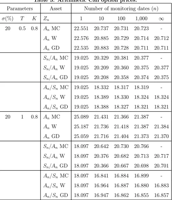
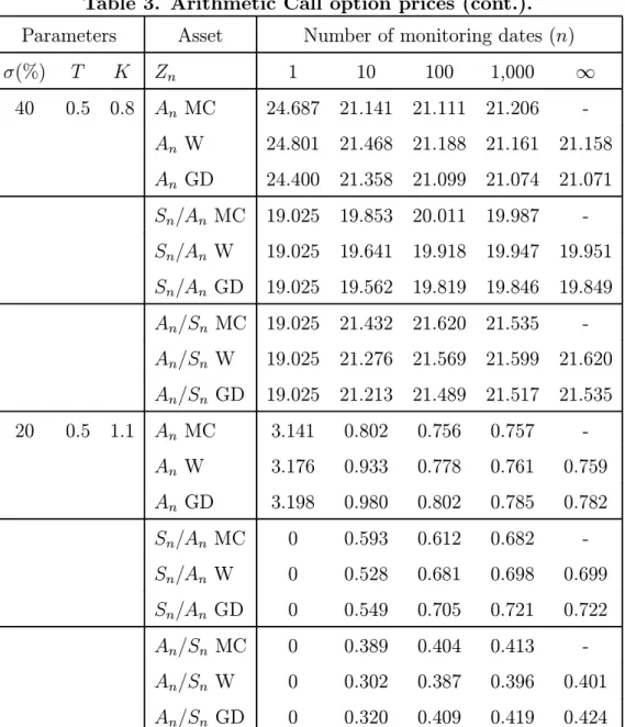
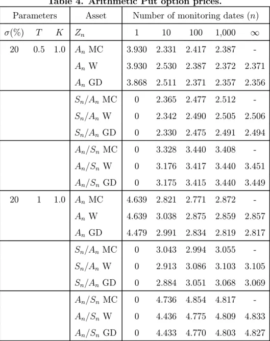
Tables 3 and 4 show arithmetic call and put option prices (multiplied by 100) for different monitoring dates. The interest rate is 10 % and the stock dividend yield is 3 %. We price options on An, Sn/An and An/Sn with three
methods: Monte Carlo simulation,14 Wilkinson approximation, and gamma distribution.
[ Insert Tables 3 and 4 about here ]
In the tables, we see that derivative prices with the three methods are very close. For example, in Table 3 we have that whenσ = 0.20, T = 0.5, K = 0.8, and n= 1,000, the values of call options on An/Sn are 18.319, 18.324, and
To price options on Sn/An with both the Wilkinson approximation and
the gamma distribution, we have computed its moments using the approx-imation of Mood et al (1974). In the tables we see that those prices are very similar to the ones obtained with Monte Carlo, so that the approxima-tions seem to work pretty well. For example, in Table 3 we see that when
σ = 0.2, T = 0.5, K = 0.8, andn= 1,000, the values of call options using the Wilkinson approximation and the gamma distribution are 20.375 and 20.374, respectively, while the value obtained with Monte Carlo simulation is 20.377. When the average is computed in continuous time (number of monitoring dates = ∞) we cannot use Monte Carlo simulation. However, as mentioned before, using 1,000 monitoring dates produces option prices very similar to those using continuous average. In Table 4 we see that the values of put options on Sn/An using the Wilkinson approximation and the gamma
distri-bution are 8.863 and 8.887, respectively, for both 1,000 and ∞ monitoring dates.
To understand better why the three method produce very similar results, we plot the risk-neutral probability density function of the arithmetic stock price average in Figure 6.
[ Insert Figure 6 about here ]
The parameter values are: r= 0.1, q = 0,σ = 0.2, T = 1, S0 = 100 and
n=∞. The expected value of the average price is 105.17, and the variance 152.74. For n = ∞ the true density function is reciprocal gamma, with parameters α= 74.42 and β = 1.29E-4. This function is approximated with a lognormal distribution with the same moments. The density function is
also estimated with Monte Carlo simulation, using a set of 50 runs of 10,000 paths with 1,000 time steps. We see that, for the parameter values used, the density functions are remarkably similar, hence the price of options on arithmetic stock prices must be close.
6
Conclusions
Australian Asian options are options on the ratio of the stock price to its average or viceversa. They show up in variable purchase options, recently studied by Handley (2000).
If the stock price follows a geometric Brownian motion and the average is defined on geometric basis, these ratios also follow a geometric Brownian motion. Thus, we are able to obtain closed-form expressions for the price of the options. However, when the average is defined on arithmetic basis, the risk-neutral distributions of these ratios at maturity are unknown. Hence, to price the options we use a particular case of Edgeworth expansion (known as Wilkinson approximation) as well as a gamma approximation (following Milevsky and Posner (1998)). We compare the results with those obtained with Monte Carlo simulations, and wefind that option prices are very similar in the three cases.
Appendix
Proof of Lemma 11. For proving expressions (2)-(3), see Johnson and Kotz (1970), p. 115. As X−1 =e−Y, application of (2)-(3) gives E(X−1) = exp ½ −m+1 2s 2¾ =e−2mE(X) V(X−1) = [E(X−1)]2hes2 −1i
2. Consider the variable
˜ X= X if X ≥K 0 if X < K , K ∈IR+
Using (1), the expectation of this variable is
E( ˜X) = Z ∞ K 1 s√2πexp − 1 2 Ã lnx−m s !2 dx
Defining the variable
y= lnx−m s , a little algebra leads to
E( ˜X) =E(X)N(s−D)
whereN(.) denotes the distribution function of a standard normal vari-able and D = lnK−m
Proof of Lemma 3
The expressions for the mean and variance follow from straightforward application of (2)-(3) in Lemma 1 to St as given by (12).
To obtain Cov(Zt, Zs), we assume s < t. We first compute E(ZtZs):
E(ZtZs) = Z02E µ exp ½µ αZ− 1 2σ 2 Z ¶ (t+s) +σZ(Wt+Ws) ¾¶ = Z02exp ½µ αZ− 1 2σ 2 Z ¶ (t+s) + 1 2σ 2 ZV(Wt+Ws) ¾ = Z02exp ½µ αZ− 1 2σ 2 Z ¶ (t+s) + 1 2σ 2 Z(t+s+ 2s) ¾ = Z02exp{αZ(t+s) +σ2Zs}
where we have used (2) in Lemma 1. Then,
Cov(Zt, Zs) = E(ZtZs)−E(Zt)E(Zs) =Z02e
αZ(t+s)+σ2 Zs− ³ Z0eαZt ´ (Z0eαZs) = Z02eαZ(t+s)heσ2Zs−1 i
Proof of Proposition 1
We split the option payoff in two components:
1. The “contingent exercise payment”, a claim with payoff
C1(Z, T, T.K) =−K I{ZT≥K} = −K if ZT ≥K 0 if ZT < K
2. The “contingent receipt of the stock”, a claim with payoff
C2(Z, T, T, K) = ZT I{ZT≥K} = ZT if ZT ≥K 0 if ZT < K
We will compute the two components of the option:
C1(Z,0, T, K) = E h e−rTC1(Z, T, T, K)|Ft i =−Ke−rT P(ZT ≥K)(49) C2(Z,0, T, K) = E h e−rTC2(Z, T, T, K)|Ft i =e−rT E[ZT |ZT ≥K] (50) Equation (8) implies ln³e−αZTE(Z T)/ZT ´ +³αZ−12σ2Z ´ T σZ √ T ∼N(0,1)
and, then, it is verified that
P(ZT ≥K) =N(d2) (51) where d2 = ln(e−αZTE(Z T)/K) + ³ αZ− 12σZ2 ´ T σZ √ T
Part 2 in Lemma 1 and a little algebra leads to
E[ZT |ZT ≥K] =E(ZT)N(d1) (52)
where d1 =d2+σZ √
T.
Including (51)-(52) into (49)-(50), we obtain the final expression for the option price.
Proof of Lemma 4 Forn≥2, we have V à n X i=1 Wti ! = V Ãn−1 X i=1 Wti+Wtn ! = V Ãn−1 X i=1 Wti ! +tn+ 2 nX−1 i=1 Cov(Wti, Wtn) = V Ãn−1 X i=1 Wti ! +n∆t+ 2 nX−1 i=1 i∆t = V Ãn−1 X i=1 Wti ! +n2∆t By induction, we get V à n X i=1 Wti ! = n X i=1 i2 ∆t= (n+ 1) ³ n+12´n 3 ∆t V à n Wtn − n X i=1 Wti ! = V(n Wtn) +V à n X i=1 Wti ! −2Cov à n Wtn, n X i=1 Wti ! = n2V(Wtn) + (n+ 1)³n+1 2 ´ n 3 ∆t−2n n X i=1 Cov (Wtn, Wti) = n2tn+ (n+ 1)³n+ 12´n 3 ∆t−2n n X i=1 ti = n2 + (n+ 1) ³ n+12´ 3 −2 n X i=1 i n∆t = (n−1) ³ n−12´n 3 ∆t
Proof of Proposition 2
These formulae are consequence of Proposition 1 and the moments of Zn
that we get now:
• Departing from (13) and applying (2)-(3) in Lemma 1 and Lemma 4, we obtain the moments of Gn.
• The same procedure applied to (14) provides the moments of Sn/Gn. • Comparing (14) and (15) and applying (4)-(5) in Lemma 1, we obtain
Proof of Lemma 5 V ÃZ T 0 Wtdt ! = E ÃZ T 0 Wtdt !2 − à E ÃZ T 0 Wtdt !!2 = E ÃZ T 0 Wtdt !2 =EÃZ T 0 Wtdt Z T 0 Wsds ! = E ÃZ T 0 Wt ÃZ T 0 Wsds ! dt ! =E ÃZ T 0 Z T 0 WtWsds dt ! = Z T 0 Z T 0 E(WtWs)ds dt= Z T 0 Z T 0 Cov(WtWs)ds dt = Z T 0 Z t 0 Cov(WtWs)ds dt+ Z T 0 Z T t Cov(WtWs)ds dt = Z T 0 Z t 0 sds dt+ Z T 0 Z T t tds dt = T 3 3 V à T WT − Z T 0 Wtdt ! = V(T WT) +V ÃZ T 0 Wtdt ! −2Cov à T WT, Z T 0 Wtdt ! = T2T + T 3 3 −2T Z T 0 Cov(WT, Wt)dt = 4T 3 3 −2T Z T 0 tdt = T 3 3
Proof of Proposition 3
These formulae are consequence of Proposition 1 and the moments ofZT
that we obtain now:
• Departing from (16) and applying (2)-(3) in Lemma 1 and Lemma 5, we obtain the moments of GT.
• The same procedure applied to (17) provides the moments of ST/GT. • Comparing (17) and (18) and applying (4)-(5) in Lemma 1, we obtain
Proof of Lemma 6
Using (12) and a little algebra, we have, fora, b, k∈IR, E(SiaSjbSnk) = S0a+b+kE µ exp ½µ r−q− 1 2σ 2¶ (ati+btj +ktn) +σ(aWti +bWtj+kWtn) ¾¶ = S0aexp ½µ r−q+a−1 2 σ 2 ¶ ai∆t ¾ S0bexp (à r−q+b−1 2 σ 2 ! bj∆t ) ×S0kexp (à r−q+k−1 2 σ 2 ! kn∆t ) exp{abσ2min{i, j}∆t} ×exp{kσ2(ai+bj)∆t} (53)
Several particular cases are the following: b=k= 0 ⇒ E(Sia) =S0aexp ½µ r−q+ a−1 2 σ 2 ¶ ai∆t ¾ a=k= 0 ⇒ E(Sjb) =S0bexp (Ã r−q+ b−1 2 σ 2 ! bj∆t ) a=b= 0 ⇒ E(Snk) =S0kexp (Ã r−q+ k−1 2 σ 2 ! kn∆t )
Plugging these expressions into (53), we get
E(SiaSjbSnk) = E(Sia)E(Sjb)E(Snk) exp{abσ2min{i, j}∆t}exp{kσ2(ai+bj)∆t} For k= 0, we get
E(SiaSjb) =E(Sia)E(Sjb) exp{abσ2min{i, j}∆t} (54)
and, then,
E(SiaSjbSnk) =E(SiaSbj)E(Snk) exp{kσ2(ai+bj)∆t} (55) Using (54) with a = 1, b = k and (55) with a = b = 1, we obtain E(SiSjk)
• Mean of AnSnk E(AnSnk) = E Ã 1 n n X i=1 SiSnk ! = 1 n n X i=1 E(SiSnk)
Using (29) with j =n, we have
E(AnSnk) = 1 n n X i=1 E(Si)E(Snk)e kσ2i∆t = 1 nE(S k n) n X i=1 S0e(r−q+kσ 2)i∆t = S0 n E(S k n)h1(r∗)
with h1(.) as given by (33) and r∗ =r−q+kσ2.
• Mean of A2 nSnk E(A2nSnk) = E Ã 1 n n X i=1 Si !2 Snk = µ1 n ¶2 E n X i,j=1 SiSjSnk = µ1 n ¶2 Xn i,j=1 E(SiSjSnk) = µ1 n ¶2 E(Snk) n X i,j=1 E(SiSj)ekσ 2(i+j)∆t (56)
where the last equation results from (30). We define zn∗ = n X i,j=1 E(SiSj)ekσ 2(i+j)∆t Then, we have zn∗ = nX−1 i,j=1 E(SiSj)ekσ 2(i+j)∆t + 2 n X i=1 E(SiSn)ekσ 2(i+n)∆t −E(SnSn)e2kσ 2n∆t = z∗n−1+ 2 n X i=1 E(Si)E(Sn)eσ 2i∆t ekσ2(i+n)∆t−E(Sn2)e2kσ 2n∆t
After some algebra, we get the recurrence law zn∗ =zn∗−1+S02h2f1(r∗+σ2) ³ e(2r∗+σ2)n∆t−er∗n∆t´−e(2r∗+σ2)n∆ti (57) If we compute z∗
1 either by its definition or using (57) and compare
both results, we obtain z∗
0 = 0.
Using (57) for different values of n, we obtain
zn∗ =S02
h
2f1(r∗+σ2)(h1(2r∗+σ2)−h1(r∗))−h1(2r∗ +σ2)
i
Plugging this expression into (56), we have E(A2nSnk) = µS 0 n ¶2 E(Snk)[2f1(r∗+σ2)(h1(2r∗+σ2)−h1(r∗))−h1(2r∗+σ2)]
Proof of Lemma 7
1. Moments of the arithmetic average An
(a) Mean of An:
Apply (31) with k= 0. (b) Covariance of An with Sn:
Apply (31) fork = 1 and (36). (c) Variance of An:
Apply (32) fork = 0 and (36). 2. Moments of the variable Sn/An:
Apply part 2 in Lemma 2 with X =Sn, Y =An.
3. Moments of the variable An/Sn
(a) Mean of An/Sn:
Apply (28) fori=n, k=−1 and (31) fork =−1. (b) Variance of An/Sn:
Proof of Remark 1
1. Replace r=q−σ2 into (36)-(37) to obtain E(An) and Cov(An, Sn).
To compute V(An), we will need the following relationships, satisfied
by the functions h1(.) and f1(.) (see (33)-(34)):
h1(−a) = exp{−(n+ 1)a∆t}h1(a) (58)
f1(−a) = −exp{−a∆t}f1(a) (59)
1 +h1(a) = f1(−a) h 1−e(n+1)a∆ti (60) f1(b) = exp{(b−a)∆t} ea∆t −1 eb∆t−1f1(a) (61)
Looking at (38), we need to compute
f1(r−q+σ2)[h1(2(r−q) +σ2)−h1(r−q)]
Defining x=r−q+σ2 and using (61), this expression becomes f1(x)f1(x−σ2) " ex∆t e (x−σ2)∆t −1 e(2x−σ2)∆t −1 ³ e(2x−σ2)n∆t−1´−³e(2x−σ2)∆t−1´ #
Taking limits when x → 0 and applying (59) and some algebra, we obtain
f1(σ2)
h
h1(−σ2)−ne−(n+1)σ
2∆ti
Replacing this result into (38) and using (58) and (60), we obtain V(An) = µS 0 n ¶2 f1(σ2)e−(n+1)σ 2∆t [h1(σ2)−2n+h1(−σ2)]
It can be seen that, as expected, this variance is positive since h1(σ2)−2n+h1(−σ2) = 2 n X i=1 ³ cosh(σ2i∆t)−1´>0
2. Replace r=q+σ2 into (39) and use h
1(0) =nto obtain E(An/Sn).
To compute V(An/Sn), looking at (40), we need to compute
f1(r−q−σ2)[h1(2(r−q)−3σ2)−h1(r−q−2σ2)]
Defining x=r−q−σ2 and applying the same procedure as in part 2
of this remark, this expression becomes f1(σ2)
h
h1(−σ2)−ne−(n+1)σ
2∆ti Replacing this result into (40) and using (58), we obtain
V µA n Sn ¶ = µ1 n ¶2h (2f1(σ2)−1) ³ e−σ2∆th1(σ2)−n ´ −n(n−1)i
Proof of Lemma 8 • Mean of ATSTk E(ATSTk) =E Ã 1 T Z T 0 Stdt S k T ! = 1 T Z T 0 E(StS k T)dt
Using (29) with j =n, we have E(ATSTk) =
1 T
Z T 0
E(St)E(STk) exp{kσ 2t }dt = 1 TE(S k T) Z T 0 S0exp{(r−q)t}exp{kσ 2t }dt = S0 T E(S k T)Φ(r∗)
with Φ(.) as given by (43) andr∗ =r−q+kσ2.
• Mean of A2 TSTk
Proof of Lemma 9
1. Moments of the arithmetic average AT
(a) Mean of AT:
Apply (41) with k= 0.
(b) Covariance of AT with ST:
Apply (41) fork = 1 and (44). (c) Variance of AT:
Apply (42) fork = 0 and (44). 2. Moments of the variable ST/AT
Apply part 2 in Lemma 2 with X =ST, Y =AT.
3. Moments of the variable AT/ST
(a) Mean of AT/ST
Apply (28) fori=n, k=−1 and (41) fork =−1. (b) Variance of AT/ST
Proof of Remark 2
1. Replace r=q−σ2 into (44)-(45) to obtain E(A
T) and Cov(AT, ST).
To compute V(AT), looking at (46), we need to compute
lim
r→q−σ2
Φ(2(r−q) +σ2)
−Φ(r−q) r−q+σ2
that is easily computed applying the L’Hˆopital’s rule. Plugging this re-sult into (46) and using the relationship Φ(−x) =e−xTΦ(x), we obtain
V(AT) = µS 0 T ¶2 e−σ2T σ2 [Φ(σ 2) −2T +Φ(−σ2)]
It can be seen that, as expected, this variance is positive since Φ(σ2)−2T +Φ(−σ2) = 2
σ2[sinh(σ 2T)
−σ2T]>0
2. Replace r=q+σ2 into (47) and use Φ(0) =T to obtain E(A
T/ST).
To compute V(AT/ST), looking at (48), we need to compute
lim
r→q+σ2
Φ(2(r−q)−3σ2)
−Φ(r−q−2σ2)
r−q−σ2
Applying the L’Hˆopital’s rule and plugging the result into (48), we obtain V µA T ST ¶ = µ1 T ¶2" 2 Φ(σ 2) −T σ2 −T 2 #
References
[1] Alziari, B., J.P. Decamps and P.F. Koehl (1997). A P.D.E. Ap-proach to Asian options: Analytical and Numerical Evidence. Journal of Banking and Finance, 21, 5, 613—640.
[2] Armata, K. (2001). Closed Form Solutions for Pricing Asian Options, mimeo.
[3] Bouaziz, L., E. Briys and M. Crouhy (1994). The pricing of forward-starting asian options.Journal of Banking and Finance, 18, 5, 823—839.
[4] Carverhill, A.P. and L.J. Clewlow (1990). Flexible Convolution. Risk, 3, 4, 25—29.
[5] Chung, S.L., M. Shackleton, and R. Wojakowski (2001). Effi-cient Quadratic Approximation of Floating Strike Asian Option Values, mimeo.
[6] Corwin, J., P.P. Boyle and K. Tan (1996). Quasi Monte Carlo Methods in Numerical Finance.Management Science, 42, 926— 938.
[7] Curran, V. (1994). Valuing Asian Options and Portfolio Options by Conditioning on the Geometric Mean Price. Management Science, 40, 12, 1705—1711.
[8] De Schepper, A., M. Teunen and M. Goovaerts (1994). An An-alytical Inversion of a Laplace Transform Related to Annuities Certain. Insurance: Mathematics and Economics, 14, 33—37. [9] Dewynne, J. and P. Wilmott (1995a). Asian Options as Linear
Complementary Problems: Analysis and Finite Difference So-lutions.Advances in Futures and Options Research, 8, 145—173. [10] Dewynne, J. and P. Wilmott (1995b). A Note on Average Rate Options with Discrete Sampling.SIAM Journal of Applied Mathematics, 55, 1, 267—276.
[11] Dinenis, E., D. Flamouris and J. Hatgioannies (2001). Valuing Exotic Options with Jump Diffusion Models: The Case of Asian Options, mimeo.
[12] Dufresne, D. (2000). Laguerre Series for Asian and Other Op-tions. Mathematical Finance, 10, 4, 407—428.
[13] Eydeland, A. and H. Geman (1995). Domino Effect: Inverting the Laplace Transform.Risk, 8, 4, 65—67.
[14] Fu, M.C., D.B. Madan and T. Wang (1999). Pricing Continu-ous Asian Options: A Comparison of Monte Carlo and Laplace Transform Inversion Methods. Journal of Computational Fi-nance, 2, 49—74.
[15] Geman, H. and M. Yor (1993). Bessel Prices, Asian Options and Perpetuities. Mathematical Finance, 3, 4, 349—375.
[16] Handley, J.C. (2000). Variable Purchase Options. Review of Derivatives Research, 4, 219—230.
[17] Hansen, A.T. and P.L. Jorgensen (2000). Analytical Valuation of American-Style Asian Options. Management Science, 46, 8, 1116—1136.
[18] Haykov, J. (1993). A Better Control Variate for Pricing Stan-dard Asian Options. Journal of Financial Engineering, 2, 207— 216.
[19] He, H. and A. Takahashi (1995-96). A Variable Reduction Tech-nique for Pricing Average-Rate-Options. Japanese Journal of Financial Economics, 1, 3—23.
[20] Jacques, M. (1996). On the Hedging Portfolio of Asian Options. ASTIN Bulletin, 26, 165—183.
[21] Jarrow, R. and A. Rudd (1982). Approximate Option Valua-tion for Arbitrary Stochastic Processes. Journal of Financial Economics, 10, 347—369.
[22] Johnson, N.L. and S. Kotz (1970). Continuous Univariate Distributions-1. Distributions in Statistics, John Wiley & Sons, New York.
[23] Ju, N. (1997). Fourier Transformation, Martingale, and the Pricing of Average Rate Derivatives, Ph.D. Thesis, University of California-Berkeley.
[24] Kemna, A.G.Z. and T.C.F. Vorst (1990). A Pricing Method for Options based on Average Asset Values.Journal of Banking and Finance, 14, 1, 113—129.
[25] Levy, E. (1992). Pricing European Average Rate Currency Op-tions.Journal of International Money and Finance, 11, 474—491. [26] Levy, E. and S. Turnbull (1992). Average Intelligence. Risk, 5,
2, 53—59.
[27] Majumdar, M. and R. Radner (1991). Linear Models of Eco-nomic Survival under Production Uncertainty. Economic The-ory, 1, 13—30.
[28] Merton, R. (1973). Theory of Rational Option Pricing. Bell Journal of Economics and Management Science, 4, 141—183. [29] Merton, R. (1975). An Asymptotic Theory of Growth under
Uncertainty. Review of Economic Studies, 375—393.
[30] Milevsky, M.A. and S.E. Posner (1998). Asian Options, the Sum of Lognormals, and the Reciprocal Gamma Distribution. Jour-nal of Financial and Quantitative AJour-nalysis, 33, 3, 409—422. [31] Mood, A.M, F.A. Graybill and D.C. Boes (1974). Introduction
to the Theory of Statistics, Mc-Graw Hill Series in Probability and Statistics, Third Edition, New York.
[32] Nielsen, J.A. and K. Sandmann (1996). The Pricing of Asian Options under Stochastic Interest Rates.Applied Mathematical Finance, 3, 209—236.
[33] Nielsen, J.A. and K. Sandmann (1998). Asian Exchange Rate Options under Stochastic Interest Rates: Pricing as a Sum of Delayed Payment Options, mimeo.
[34] Nielsen, J.A. and K. Sandmann (1999). Pricing of Asian Ex-change Rate Options under Stochastic Interest Rates as a Sum of Delayed Payment Options, Technical Report, Department of Mathematical Sciences, University of Aarhus
[35] Nielsen, J.A. and K. Sandmann (2001). Pricing Bounds on Asian Options, mimeo.
[36] Posner, S.E. and M.A. Milevsky (1998). Valuing Exotic Options by Approximating the spd with Higher Moments. Journal of Financial Engineering, 7, 109—125.
[37] Ritchken, P., L. Sankarasubramaniyan and A.M. Vijh (1993). The Valuation of Path Dependent Contracts on the Average. Management Science, 39, 10, 1202—1213.
[38] Rogers, L.C.G. and Z. Shi (1995). The Value of an Asian Option. Journal of Applied Probability, 32, 1077—1088.
[39] Shirakawa, H. (1999). Evaluation of the Asian Option by the Dual Martingale Measure. Asian-Pacific Financial Markets, 6, 183—194.
[40] Shreve, S.E. and J. Ve˜cer (2000). Options on a Traded Account, Vacation Calls, Vacation Puts and Passport Options, Working paper, Carnegie Mellon University.
[41] Stuart, A. and J.K. Ord (1987). Kendall’s Advanced Theory of Statistics, Vol. I, Distribution Theory, Charles Griffin & Com-pany Limited, Fifth Edition, London.
[42] Turnbull, S.M. and L. M. Wakeman (1991). A Quick Algorithm for Pricing European Average Options.Journal of Financial and Quantitative Analysis, 26, 3, 377 —389.
[43] V´azquez-Abad, F. and D. Dufresne (1998). Accelerated Simu-lation for Pricing Asian Options, invited paper, Winter Simula-tion Conference Proceedings, 1493—1500.
[44] Vorst, T.C.F. (1990). Analytic Boundaries and Approximations of the Prices and Hedge Ratios of Average Exchange Rate Op-tions. Working Paper, Econometric Institute, Erasmus Univer-sity, Rotterdam.
[45] Vorst, T.C.F. (1992). Prices and Hedge Ratios of Average Ex-change Rate Options. International Review of Financial Anal-ysis, 1, 3, 179—193.
[46] Vorst, T.C.F. (1996). Averaging Options. InHandbook of Exotic Options, ed. by I. Nielken, Honeywood, Il, Irwin, 175—199. [47] Yor, M. (1992). On some Exponential Functionals of Brownian
[48] Yor, M. (1993). From Planar Brownian Windings to Asian Op-tions. Insurance, Mathematics and Economics, 13, 23—34. [49] Zvan, R., A. Forsyth and K.R. Vetzal (1998). Robust Numerical
Methods for PDE models of Asian Options.Journal of Compu-tational Finance, 1, 2, 39—78.
Footnotes
1. For several examples in the real life, see Bouazizet al(1994) and Vorst (1996).
2. This is one of the main assumptions in the Black-Scholes model. See Armata (2001) or Dinenis et al (2001) for valuation of Asian options outside the Black-Scholes framework.
3. As will be indicated later, the distribution of the continuous-time average is known, allowing us to obtain exact analytical expressions for option prices.
4. It may be worth noting that if these variables were perfectly correlated, then the average would be lognormal. Alternatively, if these variables are i.i.d., applying the central limit theorem, the distribution of the average would converge to the normal one.
5. Other examples are Dewynne and Wilmott (1995a, 1995b), He and Takahashi (1995-96), Zvanet al(1998) or Shreve and Ve˜cer (2000).
6. See also Haykov (1993), Corwinet al(1996) and Nielsen and Sandmann (1996).
7. See, for example, Levy (1992), Hansen and Jorgensen (2000) and Dinenis et al (2001).
8. Merton (1975) and Majumdar and Radner (1991) are examples of papers in the economic literature that deal with the gamma distribution.
9. For completeness, this table includes the geometric average.
10. Recall that these prices have been multiplied by 100.
11. For completeness, this table includes the stock price and its geometric average. The formula for the geometric Asian option was first derived by Kemna and Vorst (1990).
12. It can be shown that for σ large enough (σ > p6/5p2Tln(S0) + 3(r−q)), this expected value is higher than E(ST).
13. Analogous notation is employed for the approximating distributionA.
Table 1. Geometric Call option prices.
Parameters Asset Number of monitoring dates (n)
σ(%) T K Zn 1 10 100 1,000 ∞ 20 0.5 0.8 Sn 22.576 22.576 22.576 22.576 22.576 Gn 22.576 20.696 20.561 20.548 20.546 Sn/Gn 19.025 20.400 20.531 20.545 20.546 Gn/Sn 19.025 18.133 18.161 18.166 18.166 20 1 0.8 Sn 25.187 25.187 25.187 25.187 25.187 Gn 25.187 21.361 21.084 21.056 21.053 Sn/Gn 18.097 20.756 21.023 21.050 21.053 Gn/Sn 18.097 16.491 16.580 16.593 16.594 40 0.5 0.8 Sn 24.801 24.801 24.801 24.801 24.801 Gn 24.801 20.766 20.558 20.538 20.536 Sn/Gn 19.025 20.332 20.514 20.534 20.536 Gn/Sn 19.025 20.266 20.908 20.979 20.987 20 0.5 1.1 Sn 3.175 3.175 3.175 3.175 3.175 Gn 3.175 0.905 0.737 0.721 0.719 Sn/Gn 0 0.549 0.701 0.717 0.719 Gn/Sn 0 0.282 0.374 0.384 0.385
Prices are multiplied by 100. The interest rate is 10% and the dividend yield 3%. For options onSn andGnwe takeS0 = 1. For options onGn, derivative
prices can be computed with the Merton’s (1973) formula when n= 1, and with the Kemna and Vorst’s (1990) formula when n=∞.
Table 2. Geometric Put option prices.
Parameters Asset Number of monitoring dates (n)
σ(%) T K Zn 1 10 100 1,000 ∞ 20 0.5 1.0 Sn 3.930 3.930 3.930 3.930 3.930 Gn 3.930 2.591 2.439 2.423 2.422 Sn/Gn 0 2.250 2.405 2.420 2.422 Gn/Sn 0 3.321 3.516 3.535 3.537 20 1 1.0 Sn 4.639 4.639 4.639 4.639 4.639 Gn 4.639 3.135 2.955 2.937 2.935 Sn/Gn 0 2.732 2.915 2.933 2.935 Gn/Sn 0 4.724 4.976 5.000 5.002 40 0.5 1.0 Sn 9.277 9.277 9.277 9.277 9.277 Gn 9.277 6.149 5.763 5.724 5.719 Sn/Gn 0 5.283 5.676 5.715 5.719 Gn/Sn 0 5.314 5.493 5.508 5.510 20 0.5 1.1 Sn 9.300 9.300 9.300 9.300 9.300 Gn 9.300 8.753 8.712 8.714 8.713 Sn/Gn 9.512 8.688 8.710 8.713 8.713 Gn/Sn 9.512 10.691 10.759 10.765 10.766
Prices are multiplied by 100. The interest rate is 10% and the dividend yield 3%. For options onSn andGnwe takeS0 = 1. For options onGn, derivative
prices can be computed with the Merton’s (1973) formula when n= 1, and with the Kemna and Vorst’s (1990) formula when n=∞.
Table 3. Arithmetic Call option prices.
Parameters Asset Number of monitoring dates (n)
σ(%) T K Zn 1 10 100 1,000 ∞ 20 0.5 0.8 An MC 22.551 20.737 20.731 20.723 -An W 22.576 20.885 20.729 20.714 20.712 An GD 22.535 20.883 20.728 20.711 20.711 Sn/An MC 19.025 20.329 20.381 20.377 -Sn/An W 19.025 20.209 20.360 20.375 20.377 Sn/An GD 19.025 20.208 20.358 20.374 20.375 An/Sn MC 19.025 18.332 18.317 18.319 -An/Sn W 19.025 18.389 18.330 18.324 18.324 An/Sn GD 19.025 18.388 18.327 18.321 18.321 20 1 0.8 An MC 25.089 21.431 21.366 21.387 -An W 25.187 21.736 21.418 21.387 21.384 An GD 25.059 21.716 21.404 21.373 21.370 Sn/An MC 18.097 20.642 20.730 20.766 -Sn/An W 18.097 20.376 20.682 20.713 20.717 Sn/An GD 18.097 20.366 20.667 20.698 20.701 An/Sn MC 18.097 16.841 16.884 16.899 -An/Sn W 18.097 16.964 16.887 16.880 16.883 An/Sn GD 18.097 16.947 16.862 16.855 16.857
Prices are multiplied by 100. The interest rate is 10% and the dividend yield 3%. For options onAnwe takeS0 = 1. MC, W and GD refer to Monte Carlo
Table 3. Arithmetic Call option prices (cont.).
Parameters Asset Number of monitoring dates (n)
σ(%) T K Zn 1 10 100 1,000 ∞ 40 0.5 0.8 An MC 24.687 21.141 21.111 21.206 -An W 24.801 21.468 21.188 21.161 21.158 An GD 24.400 21.358 21.099 21.074 21.071 Sn/An MC 19.025 19.853 20.011 19.987 -Sn/An W 19.025 19.641 19.918 19.947 19.951 Sn/An GD 19.025 19.562 19.819 19.846 19.849 An/Sn MC 19.025 21.432 21.620 21.535 -An/Sn W 19.025 21.276 21.569 21.599 21.620 An/Sn GD 19.025 21.213 21.489 21.517 21.535 20 0.5 1.1 An MC 3.141 0.802 0.756 0.757 -An W 3.176 0.933 0.778 0.761 0.759 An GD 3.198 0.980 0.802 0.785 0.782 Sn/An MC 0 0.593 0.612 0.682 -Sn/An W 0 0.528 0.681 0.698 0.699 Sn/An GD 0 0.549 0.705 0.721 0.722 An/Sn MC 0 0.389 0.404 0.413 -An/Sn W 0 0.302 0.387 0.396 0.401 An/Sn GD 0 0.320 0.409 0.419 0.424
Prices are multiplied by 100. The interest rate is 10% and the dividend yield 3%. For options onAnwe takeS0 = 1. MC, W and GD refer to Monte Carlo
Table 4. Arithmetic Put option prices.
Parameters Asset Number of monitoring dates (n)
σ(%) T K Zn 1 10 100 1,000 ∞ 20 0.5 1.0 An MC 3.930 2.331 2.417 2.387 -An W 3.930 2.530 2.387 2.372 2.371 An GD 3.868 2.511 2.371 2.357 2.356 Sn/An MC 0 2.365 2.477 2.512 -Sn/An W 0 2.342 2.490 2.505 2.506 Sn/An GD 0 2.330 2.475 2.491 2.494 An/Sn MC 0 3.328 3.440 3.408 -An/Sn W 0 3.176 3.417 3.440 3.451 An/Sn GD 0 3.175 3.415 3.440 3.449 20 1 1.0 An MC 4.639 2.821 2.771 2.872 -An W 4.639 3.038 2.875 2.859 2.857 An GD 4.479 2.991 2.834 2.819 2.817 Sn/An MC 0 3.043 2.994 3.055 -Sn/An W 0 2.913 3.086 3.103 3.105 Sn/An GD 0 2.884 3.051 3.068 3.069 An/Sn MC 0 4.736 4.854 4.817 -An/Sn W 0 4.436 4.775 4.809 4.833 An/Sn GD 0 4.433 4.770 4.803 4.827
Prices are multiplied by 100. The interest rate is 10% and the dividend yield 3%. For options onAnwe takeS0 = 1. MC, W and GD refer to Monte Carlo
Table 4. Arithmetic Put option prices (cont.).
Parameters Asset Number of monitoring dates (n)
σ(%) T K Zn 1 10 100 1,000 ∞ 40 0.5 1.0 An MC 9.277 5.465 5.402 5.554 -An W 9.277 5.874 5.525 5.490 5.487 An GD 8.971 5.792 5.457 5.423 5.419 Sn/An MC 0 5.855 6.000 5.988 -Sn/An W 0 5.837 6.202 6.238 6.242 Sn/An GD 0 5.794 6.147 6.182 6.186 An/Sn MC 0 5.078 5.202 5.201 -An/Sn W 0 4.880 5.193 5.224 5.290 An/Sn GD 0 4.822 5.124 5.154 5.217 20 0.5 1.1 An MC 9.300 8.571 8.581 8.576 -An W 9.300 8.613 8.589 8.588 8.588 An GD 9.322 8.639 8.613 8.611 8.611 Sn/An MC 9.512 8.838 8.827 8.829 -Sn/An W 9.512 8.858 8.862 8.863 8.863 Sn/An GD 9.512 8.879 8.886 8.887 8.887 An/Sn MC 9.512 10.586 10.626 10.617 -An/Sn W 9.512 10.453 10.603 10.618 10.623 An/Sn GD 9.512 10.472 10.625 10.640 10.646
Prices are multiplied by 100. The interest rate is 10% and the dividend yield 3%. For options onAnwe takeS0 = 1. MC, W and GD refer to Monte Carlo
0 10 20 30 40 50 0 0.005 0.01 0.015 0.02 0.025 0.03 0.035 0.04 0.045
Number of monitoring dates
Logarithmic Variance
Figure 1: Plot of the logarithmic variance (σ2
ZT) as function of n.
The parameter values are σ = 0.2 and T = 1. The figure depicts the loga-rithmic variance of the stock price (dotted line), Gn (dashed line), GT (solid
line),Sn/Gn (dotted-dashed line), andGn/Sn. These values are given by the
following table: Zn σZ2T Sn σ2T Gn (n+1)(n+1 2) 3n2 σ 2T Sn/Gn (n−1)(n−1 2) 3n2 σ 2T Gn/Sn (n−1)(n−1 2) 3n2 σ 2T