Energy Performance and comfort in residential buildings

(1)

51 Energy Performance and comfort in residential buildings

2

Energy Performance and comfort

in residential buildings

Sensitivity for building parameters and occupancy

1

Abstract

Energy performance simulation is a generally used method for assessing the energy consumption of build-ings. Simulation tools, though, have shortcomings due to false assumptions made during the design phase of buildings, limited information on the building’s envelope and installations and misunderstandings over the role of the occupant’s behavior. This paper presents the results of a Monte Carlo sensitivity analysis on the factors (relating to both the building and occupant behavior) that affect the annual heating energy consumption and the PMV comfort index. The PMV results are presented only for the winter (heating) period, which is important for energy consumption in Northern Europe. The reference building (TU Delft Concept House) was simulated as both a Class-A and Class F dwelling and with three different heating systems. If behavioral parameters are not taken into account, the most critical parameters affecting heating consumption are the window U value, window g value and wall conductivity. When the uncertainty of the building-related parameters increases, the impact of the wall conductivity on heating consumption increases considerably. The most important finding was that when behavioral parameters like thermostat use and ventilation flow rate are added to the analysis, they dwarf the importance of the building parameters. For the PMV comfort index the most influential parameters were found to be metabolic activity and clothing, while the thermostat had a secondary impact.

§ 2.1

Introduction

Building performance simulation has been established as a widely accepted method of assessing energy consumption during the design process for buildings that are either due to be renovated or are going to be built new. Modern buildings are highly complex and have high performance requirements relating to sustainability, making simulations a necessity.

Building simulation tools have shortcomings and are unreliable at predicting the energy performance of buildings. The reasons for these failings could be technical, such as weather variations and false assumptions during the building design phase [1, 2]. Also limited information on the building’s envelope and installations (especially

1 Published as: Ioannou, A., and L. C. M. Itard. “Energy performance and comfort in residential buildings: Sensi- tivity for building parameters and occupancy.” Energy and Buildings 92 (2015): 216-233.

(2)

52 Thermal comfort and energy related occupancy behavior in Dutch residential dwellings

when the buildings are very old and there are no records of the materials used) may also play an important role in the discrepancies between simulated and actual energy use. As a result, large differences are observed between predicted and actual energy performance, ranging from 30% up as far as 100% in some cases [1-6]. In Majcen and Santin [3-5], it was also shown that predictors are much worse for buildings with a lower energy class (generally older stock) than those with a higher energy class (generally the more recently built stock). Another important reason is related to a misunderstanding or underestimation of the role of the occupant’s behavior [1, 6, 7]. Current simulation software fails to take into account the energy-related behavior of the occupant and his behavior towards indoor comfort. There are numerous studies that emphasize the need to take proper account of the occupant’s behavior during the design phase, or even during the refurbishment stage, in order to generate better building energy performance predictions [1, 2, 6, 8, 9].

The energy models that are used to predict the energy performance of buildings are sensitive to specific input parameters. These most sensitive parameters should be modelled with care in order to represent the building as accurately as possible [10-12]. Accordingly, in order to improve the quality of the prediction of building energy performance, it is important to understand its sensitivity to the various input parameters, and in this particular case, changes in a combination of the building envelope and the occupancy behavior parameters. This can be done through sensitivity analysis and specifically using the method of Monte Carlo analysis (MCA) [13].

Several studies can be found in literature with sensitivity analysis performed on the effects of technical and physical parameters on the energy consumption of buildings [12-18]. However, occupancy-related parameters that could reflect the behavioral pattern of occupants have rarely been studied and moreover, the majority of studies have involved commercial or office buildings and not residential buildings, which are the main object of the present study.

The international standard ISO 7730 is a commonly used method for predicting the thermal sensation (PMV) and thermal dissatisfaction (PPD) of people exposed to moderate thermal environments. The PMV model predicts the thermal sensation as a function of activity, clothing and the four classical thermal environmental parameters: air temperature, mean radiant temperature, air velocity and humidity. Activity means the intensity of the physical activity of a person and the clothing is the total thermal resistance from the skin to the outer surface of the clothed body. Many widely used building simulation programs such as ESP-r, TRYNSYS and Energy+ use ISO 7730 [19] to calculate comfort levels inside a building. One main criticism of the PMV/PPD method is that it disregards the effect of adaptations, the changing evaluation of the thermal environment due to changing perceptions. There are three different forms TOC

(3)

53 Sensitivity for building parameters and occupancy of adaptation, which are all interrelated and affect one another [20]. Psychological adaptation relates to a person’s thermal expectations based on his past experiences and habits [21-23]. Physiological adaptation (acclimatization), relates to how an individual adapts to a thermal environment over a period of some days or weeks and behavioral adaptation relates to all modifications or actions, which an individual might make consciously or unconsciously, and changes in the heat and mass fluxes governing the body’s thermal balance [20]. These modifications may be personal [24-26], technological, or environmental adjustments [27]. The environment inside a residential dwelling is not as constant as that of an office and the range of behavior of occupants and their interactions with building components is wider than in office buildings. All forms of thermal adaptation can be applied in residential dwellings: changing the level of activity and clothing, adjusting the thermostat, opening or closing windows and window shades, etc. It is suspected that user behavior plays a much more important role in determining the comfort range, which may also be much wider than in office buildings, which are often more uniformly conditioned by HVAC and individuals have much less potential for changes and adaptations.

There is a significant gap in the literature when it comes to sensitivity analysis of physical, technical and occupancy parameters in the residential sector of areas with a maritime climate such as the Netherlands. Few studies have evaluated these parameters with a complete sensitivity analysis method, which reflects the occupant’s energy-related behavior such as ventilation and thermostat settings as well as physical parameters for heating consumption and comfort index.

This paper presents the results of a sensitivity analysis study that was performed for a single residential housing unit in the Netherlands. The analyses were performed for the technical/physical properties of the building only- i.e. the thermal conductivity of the walls, floor and roof, window U and g values, orientation, window frame conductivity and indoor openings. The simulations were carried out with the following variations: multi-zone and single-zone versions of the building; two different grades of insulation; three different types of HVAC services; the occupant’s behavioral characteristics (thermostat level, ventilation behavior, metabolic rate, clothing and presence that in simulation terms is the heat emitted by people). The sensitivity of the above-mentioned parameters was gauged for the yearly total heating demand of the building and the hourly PMV comfort index. The present paper focuses on the heating period, which is of importance in the Netherlands.

(4)

§ 2.2

Methodology

The goal of the study is to make recommendations for

1 the effect of the accuracy of measurements relating to the building’s physical properties on predicting the energy consumption of the building;

2 We will seek to answer the following questions:

–

Which are the most critical parameters (physical and behavioral) that influence energy use in residential dwellings for heating according to whole building simulation software?

–

Which parameters have the most critical influence on the PMV comfort index?

–

How do the most important parameters for heating and PMV relate to each other?

–

Is the sensitivity different for dwellings with different physical qualities and different energy classes?

–

What do the results mean for the modelling techniques for predicting the energy consumption in dwellings (simple versus more complicated models)?

First, a sensitivity analysis will be carried out to determine the most important physical parameters for the energy consumption of the dwelling. Next, the behavioral parameters (heat emission due to tenants’ presence, thermostat and ventilation) are added to the sensitivity analysis in order to compare the effect of the physical parameters and the behavioral parameters on the total energy consumption for heating. At the same time, another sensitivity analysis will be carried out in order to assess the most important parameters for the thermal comfort index (PMV). Possible overlap between the most influential parameters for the total energy consumption and the comfort index could reveal possibilities for improvement that could lead to reduced energy consumption and higher comfort levels.

§ 2.2.1

Sensitivity Analysis

The technique of sensitivity analysis is used to assessing the thermal response of buildings and their energy consumption [13]. The goal of a sensitivity analysis is to study the response of the model simulated by EnergyPlus with respect to the variations of specific design parameters. TOC

(5)

55 Sensitivity for building parameters and occupancy

In general, a sensitivity analysis is able to determine the effect of a building’s design variable on its overall performance (for example, the demand for heating or cooling) of the building. It can be used to assess which set of parameters has the greatest influence on the building performance variance, and at what percentage. Sensitivity analyses can be grouped into three classes: screening methods, local sensitivity methods and global sensitivity methods. Screening methods are used for complex, computationally intensive situations with a large number of parameters, such as in sustainable building design. This method can identify and rank in subjective terms the design parameters that are responsible for the majority of the output variability e.g. energy performance. These methods are called OAT methods (one-parameter-at-a-time) and the impact of changing the values of each parameter is evaluated in turn (partial analysis). A performance estimation using standard values is used as control. For each design parameter, two extreme values are selected on either side of the standard value. The differences between the results obtained by using the standard value and the extreme values are compared in order to evaluate which parameters would affect the energy performance of the building the most [28]. Local sensitivity analysis methods are also based on an OAT approach, but the evaluation of output variability is based on the variation of one design parameter between a certain range (and not only on extreme values) while the rest are maintained at a constant level. This method is a useful way of comparing the relative importance of various design parameters. The input-output relationship is assumed to be linear and the correlation between design parameters is not taken into account [28].

In global sensitivity methods, output variability due to one design parameter is evaluated by varying all the other parameters at the same time, while also taking account of the effect of range and shape of their probability density function. Randomly selected design parameter values and their calculated outputs are the means for determining the design parameters’ sensitivity. The influence of other design parameters is very important in a sensitivity analysis because the overall performance of the building is determined by all these parameters and how they interact.

Distribution effects are relevant because parameter sensitivity depends not only on the range and on distribution of the individual parameter but also on other parameters, that building performance is sensitive to. Design parameter sensitivity often depends on the interaction and influence of all the design parameters [28]. The method used in the present study is the Monte Carlo analysis; this is a variance-based method and a form of global sensitivity analysis.

(6)

§ 2.2.1.1

Monte Carlo Analysis

There are several mathematical methods for sensitivity analysis that can be found in the literature [11,13,18,29-32]. The Monte Carlo analysis (MCA) method was chosen for the purposes of this study. The use of MCA in the field of thermal modelling was proposed by the employees at the SERI [33] and the Los Alamos National Laboratory [34]. Under MCA, all the uncertain parameters are assigned a definite probability distribution. For each simulation, a value is selected at random for each input based on the probability of its occurrence. For inputs that are distributed with a Gaussian (normal) distribution, a value close to the modal value is more likely to be selected than an extreme value. The predictions that are produced by this unique set of parameter values are saved and the process is repeated many times, using a different and unique set of values for each parameter every time. When the process reaches an end, all the values for the predicted parameter (e.g. energy performance or PMV) that have been calculated from each simulation are recorded. At the same time, all the values for each of the design parameters for every simulation are also recorded [13].

The accuracy of the method is based on the number of simulations that have taken place and not on the number of the uncertain input parameters. This means that given enough computational power, the effect of a large number of parameters could be assessed simultaneously with MCA. Figure 2.1 shows that irrespective of the number of parameters, only marginal improvements can be obtained after 60-80 simulations [13].

FIGURE 2.1 Relationship between normalized confidence interval and number of MC simulations (From Lomas and Eppel, 1992)

(7)

57 Sensitivity for building parameters and occupancy Since all the inputs are perturbed simultaneously, the method takes full account of any interactions between the inputs and, in particular, any synergistic effects. Moreover any non-linearity effects in the input/output relationships are fully accounted for [13].

§ 2.2.1.2

Sampling

Three sampling techniques are relevant to Monte Carlo analysis: simple random, stratified and Latin Hypercube Sampling (LHS). Random sampling is the most basic sampling technique and works by generating a random number and scaling it to the target variable via its probability distribution [35]. The stratified sampling method is an improvement on simple random sampling that force the sample to conform to the whole distribution that is being analyzed. In order to achieve this, the probability distribution of the target variable is divided between several strata of equal probability and finally, one value is chosen at random within each stratum. Latin hypercube sampling method is a further improvement on the stratified sampling method. It works by dividing the input into strata and then generating samples so that the value generated for each parameter comes from a different stratum [36]. However, stratified sampling can introduce unknown bias into the results of the analysis [37, 38] and varying degrees of success are encountered with the use of Latin hypercube sampling [29]. A study by McDonald [35], which compared all the above sampling techniques for Monte Carlo analysis, suggests that the best combination for MCA in typical building simulation applications is simple random sampling with 100 runs. For the present study, simple random sampling was therefore chosen with, for the sake of accuracy, 200 simulation runs.

§ 2.2.1.3

Statistics

The post-processing took place in SPSS [39] after each of the 200 simulation sets was finished and the results were recorded. The use of the regression analysis enabled us to calculate the sensitivity ranking based on the relative magnitude of the regression coefficients. The parameters that were used in the simulations have different units and relative magnitudes and for that reason, a standardization process was needed. For this study, the standardization of the regression analysis took place in the form of transformation by ranks [40]. Moreover, the ranking of the raw data allowed the exploration of non-linear relationships between predictors and dependent variables. The regression analysis was then performed on the rank transformed data rather than the raw original ones. The beta value that was produced by the regression analysis

(8)

58 Thermal comfort and energy related occupancy behavior in Dutch residential dwellings is the standardized rank regression coefficient (SRRC). The SRRC values that were obtained are the sensitivity indicator for each parameter and describe the effect that this parameter has on the dependent variables (energy consumption for heating and PMV). Only statistically significant parameters are presented in the results, with the significance level being 0.05. The higher the value of the SRRC, the more sensitive the parameter is and thus the more impact it has on the heating energy or the PMV. A positive SRRC means that an increase in the parameter leads to an increase in the value of the dependent variables; a negative SRRC means that an increase in the parameter leads to a decrease.

§ 2.2.2

Tools

The initial modelling of the reference building was carried out using the simulation software DesignBuilder, which is a user interface for the Energy+ [41, 42] dynamic thermal simulation engine. Energy+ is a dynamic simulation software for energy analysis in buildings, which is based on transient heat conduction equations and combined heat, and mass transfer in construction elements. The building file was exported in the form of an Energy+ file and uploaded to the main Energy+ editor for the simulation of the installations. The parametric simulations for the Monte Carlo analysis took place with an Energy+ add-on that was created for that purpose, the jEPlus [43, 44].

§ 2.2.3

Reference Building

The reference building for the simulations was based on a real building, the Concept House built by TU Delft in Rotterdam. Two variations of the concept house were initially chosen as reference cases based on their energy class, which represents the amount of energy consumed per m2_{in kWh/year. Two buildings were used (external envelope} materials) corresponding to a Class-A building and a Class-F building, according to the Dutch building code ISSO 82.3 [45]. The dwelling consists of a living room with kitchen, two bedrooms, a bathroom, a storage room and a hallway. The floor area of the house is 86.2m2_{and its height is 2.7m. The shading system of both dwellings consists} of blinds with high reflectivity slats, positioned outside the window system. The blinds are open while the occupants are awake and closed when they are asleep or absent. The blinds therefore also act as window insulation.

(9)

§ 2.2.4

Independent variables and predictor parameters

The output (dependent) variables selected for this study were the total annual heating demand and hourly PMV. The first part of the study is about the first dependent variable, the annual heating. The reference building was modelled in two ways, as a single zone and as a multi-zone (three zones: kitchen/living room, bedroom 1 and bedroom 2 were the heated areas in this case). Each single zone and multi-zone model was modelled as a Class-A and Class-F buildings based on the Dutch energy labels for buildings ISSO 82.3 [45], according to European directive 2010/31/EU [46] on the energy performance of buildings.Furthermore, modelling was carried out for three different heating systems: ideal loads, high efficiency boiler with radiators and floor heating coupled with a heat pump.

The most important parameters needed for a building’s thermal simulation are the thermo-physical properties of the construction materials (conductivity, specific heat, density), the casual gains associated with occupancy and appliances and infiltration/ ventilation rates. Without those parameters, a reliable model could not have been created [37]. Previous studies have demonstrated that in simulations, the most sensitive parameters affecting the heating consumption are the conductivity of the external construction components, the outdoor temperature (as described by a weather file), equipment heat gains and the infiltration/ventilation rate [18, 37]. Furthermore occupancy could play a major role in households’ demand for energy and that the presence of a thermostat is a major factor in the demand for heating [47]. In our study, we did not consider sensitivity to outdoor temperature, as we were mainly interested in explaining the differences in sensitivity in different types of dwellings that are all located in the same climate area: the Netherlands. Furthermore, in the multi-zone model we did not take into account the air exchange between zones.

The predictor parameters for the present study were chosen in such a way that they cover all four of the parameters mentioned above, which are essential for the thermal modelling of a building. The Class-A (thermally efficient) and Class-F (thermally inefficient) reference building was simulated once with predictor variables: walls, roof and floor conductivity, window glazing U and g values, window frame thickness, building orientation. The second time, the two classes were simulated with the same set of predictor variables plus the occupant behavior related parameters of ventilation, thermostatic level and the heat emitted due to the presence of the occupant.

Figure 2.2 shows a complete picture of the simulations and combinations of the type of buildings, class of buildings and parameters used for this study. Each of the parameters was assigned a base case value and a normal probability distribution

(10)

based on which, the parameter value was randomly changing. Normal distribution maximizes the information entropy among all distributions with a known mean and standard deviation. The standard deviation was 5% of the base case value for each parameter [18, 37]. Moreover, in old buildings the accuracy of the U-value is very different from new buildings. For ventilation, it is the same. Preliminary analysis of the data justified the choice of 5%. We can guess that conductivity of walls/floor/roofs, thermostat, ventilation& infiltration, and heat emitted due to people (which as input in the simulation is translated as number of people present) have the highest standard deviation (of all parameters of Table 2.1, they are the most difficult to estimate accurately, especially in older buildings) while orientation is easy to determine. However, even when we keep the standard deviation low (5%) these parameters still appear to be the most influential. Therefore increasing their standard deviation will lead to the same trend in the results with even more influence. Table 2.1 shows the base case values (mean) of the parameters, the standard deviation and the amount of samples. Ventilation and infiltration are presented together as one number, which is the same for both reference buildings (Class-A and Class-F), because the sum of infiltration and ventilation flow rates was chosen to ensure enough fresh air. In the first case, infiltration is much lower and ventilation much greater because the Class-A building is new and airtight while in the Class-F building infiltration is higher and ventilation lower because building is older and less airtight.

TABLE 2.1 Mean, std. deviation and number of samples for the predictor parameters for total heating and cooling

PARAMETERS CLASS A CLASS F

mean std. deviation samples mean std. deviation Samples

Orientation (degrees angle) 245 14.5 10 245 14.5 10

Wall Conductivity [W/(m-K)] 0.048 0.0024 10 0.25 0.0125 10

Roof Conductivity [W/(m-K)] 0.048 0.0024 10 0.3 0.015 10

Floor Conductivity [W/(m-K)] 0.048 0.0024 10 0.3 0.015 10

Window Glazing U value [W/(m2_K] _0.96 _0.064 ₁₀ _6.121 _0.3 ₁₀

Window Glazing g value 0.5 0.03 10 0.81 0.04 10

Window Frame Thickness [m] 0.045 0.003 10 0.045 0.003 10

Thermostat [o_C] ₂₀ ₁ ₁₀ ₂₀ ₁ ₁₀

Ventilation+ Infiltration (flow rate) [m3_/s] _0.1 _0.005 ₁₀ _0.1 _0.005 ₁₀

People present (heat emitted by people) 2 0.1 10 2 0.1 10

(11)

FIGURE 2.2 Schematic representation of simulations between building types and parameters

The second part of the study related to the second dependent variable, the hourly PMV. The predictor variables used were the thermostat setting, metabolic activity, clothing, and ventilation (airflow rate), while the air speed in the rooms was held constant (0.14 m/sec). The reason for the choice of these variables was that they represent the factors that affect the thermal comfort index (PMV) most closely. The PMV model predicts the thermal sensation as a function of metabolic activity, clothing and air temperature, mean radiant temperature, air velocity and humidity [19]. In reality, air temperature and radiant temperature related to the thermostat setting, while humidity and air speed related to the ventilation of the building. However, in Energy+ the local air speed of the rooms that affects comfort is not dynamically calculated from infiltration and ventilation; instead it can only be defined using a schedule, which means that detailed and reliable comfort calculations can only take place if an extensive file with air speed patterns (produced from empirical data or from CFD calculation) is available [41, 42]. TOC

(12)

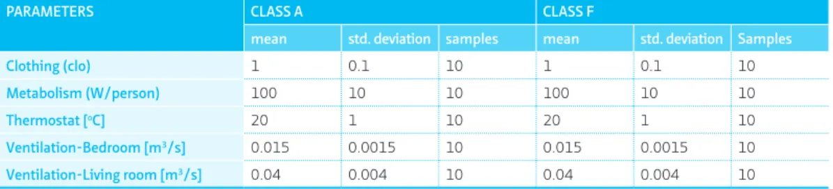
Each simulation in the first part of this study was performed for each hour of a whole year. For the second part of the study, each simulation was performed for a whole day in the fall, the winter, the spring and summer. The reason for this was that it makes no sense for the dependent variable to have a yearly PMV value. The PMV value can change many times in a day, even within one hour, and cannot be aggregated to a yearly value. Moreover, a yearly PMV value says nothing meaningful about the occupants’ feeling of comfort. Figure 2.3 shows a complete picture of the simulations and combinations of type of buildings, class of buildings and parameters that took place in the second part of this study. As in the first part of the study, each of the parameters was assigned a base case value and a normal probability distribution, based on which the parameter value changed randomly. Table 2.2 shows the base case values (mean) of the parameters, the standard deviation (10% around the mean) and the number of samples [18].

FIGURE 2.3 Schematic representation of simulations and combinations between buildings types and parameters

(13)

TABLE 2.2 Mean, std. deviation, and number of samples for the predictor parameters for hourly PMV

PARAMETERS CLASS A CLASS F

mean std. deviation samples mean std. deviation Samples

Clothing (clo) 1 0.1 10 1 0.1 10 Metabolism (W/person) 100 10 10 100 10 10 Thermostat [o_C] ₂₀ ₁ ₁₀ ₂₀ ₁ ₁₀ Ventilation-Bedroom [m3_/s] _0.015 _0.0015 ₁₀ _0.015 _0.0015 ₁₀ Ventilation-Living room [m3_/s] _0.04 _0.004 ₁₀ _0.04 _0.004 ₁₀

§ 2.2.5

Heating Systems

Both Class A and F dwellings were simulated with three different heating systems. The first heating system was based on the model of ‘’Ideal Loads Air System’’. This model can be thought of as an ideal unit that mixes the air at the zone exhaust condition with the specified amount of outdoor air and then adds or removes heat and moisture at 100% efficiency to produce a supply air stream with the properties specified [41]. The second heating system is based on the model ’’Low Temperature Radiant: Constant Flow’’ of Energy+. This low temperature radiant system (hydronic) is a component of zone equipment that is intended to model any radiant system where water is used to supply/remove energy to/from a building surface (wall, ceiling, or floor). The low temperature radiant system is supplied with warm water from a water-to-water heat pump. The supply side of the heat pump is connected to a ground heat exchanger and the circulation pump is a constant speed pump [41, 42]. This system will henceforth be referred as the floor heating system, which includes a heat pump. The third heating system is a high temperature radiant system (gas-fired) that is intended to model any ‘’high temperature’’ or ‘’high intensity’’ radiant system where electric resistance or gas-fired combustion heating is used to supply energy (radiant heat) [41]. In this model, the user is allowed to specify the fraction of heat that leaves the heater as radiation, latent heat and heat that is lost. The user can also specify the fraction of radiant heat (0.4 for this study) that reaches the occupants and the zone surfaces, which is later used in the thermal comfort calculations. Moreover, the radiant fraction of energy that reaches the occupants and the zone surfaces always sums up to unity; although every fraction of radiant energy affects the occupants in a zone, it automatically affects the zone surfaces as well. As such, there are no ‘’losses’’ from the perspective of zone air temperature and the surfaces heat balance. This system will henceforth be referred as the Radiator system, which includes the gas boiler.

(14)

§ 2.2.6

Natural Ventilation

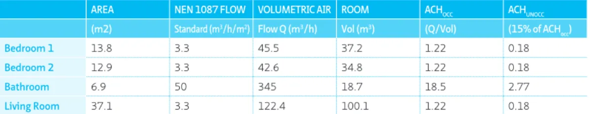
The natural ventilation for each of the thermal zones of the base case scenario is calculated from the directions given by the Dutch NEN 1087 standard. The NEN standard provides the required flow for each room. The ACH when the rooms are not occupied is set to 15% of the ACH when the room is occupied and the air exchange between zones has not been modelled. Infiltration was calculated based on the Dutch NEN 1087 [48] standard and added to the ventilation. Table 2.3 shows all the data related to the natural ventilation calculations.

TABLE 2.3 ACH (including ventilation and infiltration) per room when the space is occupied and unoccupied

AREA NEN 1087 FLOW VOLUMETRIC AIR ROOM ACHOCC ACHUNOCC (m2) Standard (m3/h/m2) Flow Q (m3/h) Vol (m3) (Q/Vol) (15% of ACH

occ)

Bedroom 1 13.8 3.3 45.5 37.2 1.22 0.18

Bedroom 2 12.9 3.3 42.6 34.8 1.22 0.18

Bathroom 6.9 50 345 18.7 18.5 2.77

Living Room 37.1 3.3 122.4 100.1 1.22 0.18

§ 2.2.7

Heating and Ventilation Controls

For all three systems, the temperature control type was the mean air temperature of the zone. The thermostatic control set point defines the ideal temperature (i.e. setting of the thermostat) in the space. During daytime and occupied periods, this heating set point is set to 20 o_{C for all rooms and for the whole year [49, 50]. Every time the} mean air temperature falls below 20 o_{C the system is providing heat to the zone, if it is} above 20 o_{C then the system will stop. The setback set point temperature, which is the} temperature during the night and unoccupied periods, is set to 16 o_{C. The thermostatic} control set point determines whether or not there is a heating load in the space and thus whether the systems should be operating.

In the ideal loads system, the control is only through the thermostatic control set point. Heating control in the high temperature radiant system (radiator + boiler) takes place with two additional parameters: the heating set-point temperatures and the throttling range. The throttling range specifies the range of temperature, in degrees centigrade,

(15)

over which the radiant system throttles from zero heat input to the zone up to the maximum. The heating set-point temperature specifies the control temperature for the radiant system in degrees centigrade and controls the flow rate to the radiant system [41, 42]. This set point is different from the thermostatic control set point for the zone. In our study, the heating set point temperature was set to 20 o_{C and the throttling} range to 1 o_C.

The control for the low temperature radiant system takes place with four additional parameters: heating high and low control temperatures and heating high and low water control temperatures. The zone mean air temperature is compared to the high and how control temperatures at any time. If the mean air temperature is higher than the high temperature, then the system will be turned off and the water mass flow rate will be zero. If the mean air temperature is below the low temperature, then the inlet water temperature is set to the high water temperature. If the mean air temperature is between the high and low value of the control temperature, then the inlet water temperature is linearly interpolated between the low and high water temperature value [41]. In our study, the heating high and low control temperatures were 21 o_{C and 18}o_C and the heating high and low water temperatures were 35 o_{C and 10}o_C.

§ 2.2.8

Activity

§ 2.2.8.1

Clothing and Metabolic Rate

There were two occupants in the dwelling, a man and a woman. The density (people/ m2_{) was thus 0.0232. The metabolic rate of the two tenants was chosen to be} ‘’Standing Relaxed’’ during the occupancy periods, which corresponds to 100 W/ person. Moreover, the metabolic factor accounts for physical size and is 1 for men and 0.85 for women. In our case, the average metabolic factor (0.90) for a man and a woman (which were assumed the occupants of the concept house) was used for the simulations.

The clothing factor (clo) was set to 1 for the whole year. Usually 0.5 is the clo value for the summer period but preliminary simulations showed that the comfort index in the Netherlands during the summer period at 0.5 clo is low, which means that the occupants would feel cold. In addition, the clothing habits of people in the Netherlands during the summer months resemble a factor closer to 1 clo than 0.5. Clothing with

(16)

factor of 1 clo corresponds to: trousers, long-sleeved shirt, long-sleeved sweater, underwear T-shirt. Summer clothing of 0.54 clo corresponds to knee-length skirt, short-sleeved shirt, panty hose, sandals [51]. Table 2.4 shows the input that was used for the simulation for the base case scenario.

TABLE 2.4 Occupancy simulation assumptions for the base case scenario

Density (people/m2₎ _0.0232

Metabolic Rate (W/person) 100 (Standing relaxed)

Metabolic Factor 0.90

Clothing factor (clo) 1

§ 2.2.8.2

Occupancy

The occupancy schedules vary according to the type of the thermal zone. In Table 2.5 we can see the occupancy for the living room/kitchen and in Table 2.6 the occupancy for the bedroom.

TABLE 2.5 Occupancy Schedule, Living Room/Kitchen

OCCUPANCY SCHEDULE--LIVING ROOM/KITCHEN MORNING EVENING

Weekdays 7:30-9:00 18:00-22:00

Saturday 9:30-11:00 18:00-22:00

Sunday 9:30-11:00 17:00-22:00

TABLE 2.6 Occupancy Schedule, Bedroom

OCCUPANCY SCHEDULE--BEDROOMS NIGHT EVENING

Weekdays 24:00-7:00 22:00-24:00

Saturday 24:00-9:00 22:00-24:00

Sunday 24:00-9:00 22:00-24:00

A half-hour gap in the occupancy of the bedrooms and living room-kitchen can be observed between 7:00 a.m. and 7:30 a.m.; this is because the occupants are assumed to use the bathroom for half an hour in the morning. The bathroom belongs to the non-heated zone.

(17)

During occupied periods, the living room and the bedrooms were assumed to have two people. For the sensitivity analysis, the number of people in the rooms was varied around the mean of two people with 0.1 (0.5% of the mean).

§ 2.2.8.3

Heat Gains

The internal gains in the dwellings for the base-case simulation scenario are due to occupancy (the heat that a person emits while in the room), a refrigerator, a computer, a monitor, a wireless router, and a television set which are all placed in the living room. Lighting is also a major contributor to the internal gains, which are set at 5 W/m2_for the whole house but with different schedules for the operation for every room. In Table 2.7 the internal gains are summarized.

TABLE 2.7 Internal heat gains: people, equipment and lighting

TYPE OF INTERNAL GAIN ACTIVITY TOTAL HEAT UNITS

Person Light Activity 126 W/person

Refrigerator Always on 3.24 W/m2 Computer + Monitor 18:00-22:00 3.78 W/m2 Television 18:00-22:00 6.75 W/m2 Router Always on 0.35 W/m2 Lighting Occupancy 5 W/m2

§ 2.3

Results

The mean and standard deviation of the total annual consumption for the various configurations of the dwellings, is displayed in Figure 2.4. The heating consumption for the ideal loads--single zone model and the multi-zone boiler/radiator model is similar for both the Class A and Class F dwellings. The consumption of the heat pump system though, appears to be much higher on both classes. The reason for that is the way that the systems are controlled. The ideal loads and radiator systems availability follows the occupancy schedules mentioned in section 2.8.2 and the rest of the hours the system is shut off or in set-back temperature during the night. The floor heating system on the

(18)

other hand is operating around the clock without intermission, and during the night, there is a setback temperature of 16 o_{C. This amounts to 168 hours per week compared} to the 49 hours of operation for the other two systems. The consumption for the ideal loads system is the total demand for a whole year, for the radiator system it includes the gas boiler combustion efficiency, which was set to 1 (high efficiency boiler) and for the floor heating system it includes the coefficient of performance that was 2.47. The high efficiency of the floor heating system compensates for a large part the higher number of hours of operation. Finally, the high consumption of the floor heating in Class F is explained in section 3.1.4. Note that a heat pump would probably never be installed in a Class F dwelling.

The results of these simulations correspond with the findings that energy savings by using air/water heat pumps are, in the Netherlands at least, often disappointing, which has among others to do with the fact that no set back temperature settings are used to avoid long periods of warming (floor heating is a slow system) that lower comfort levels [49]. 0 5000 10000 15000 20000 kWh/year

Mean and Standard Deviation

Mean and Standard Deviation--annual heating consumption

Class A--single zone Class A--multizone--radiator Class A--multizone--floor heating Class F--single zone

Class F--multizone--radiator Class F--multizone--floor heating

FIGURE 2.4 Mean and Standard Deviation for the annual heating consumption of the various heating systems

(19)

§ 2.3.1

Heating Sensitivity Analyses

§ 2.3.1.1

General Trends

Figures 2.5, 2.6, 2.7 and 2.8 show the results for the Class A and Class F buildings with and without the behavioral parameters, for both the single and multi-zone models and for three types of heating systems. Only the parameters that were found to be significant are displayed in the results. For the Class A configuration of the reference building and for all three different types of heating systems that were modelled, the most influential parameter with a positive effect (the higher the value of the parameter, the more energy is needed for heating) that affects the annual heating consumption, is the window U value (Figure 2.5). The results of the sensitivity analysis for the concept house (Figure 2.6) modelled as a Class F dwelling, showed that the window U value was not the most influential parameter. In fact, the window U-value has a very small impact on the floor heating and the ideal loads configurations, but it is insignificant for the radiator system. Wall conductivity, window g value and orientation are the most critical parameters in the Class F dwelling. Window frame thickness is insignificant in all cases.

§ 2.3.1.2

Behavioral Parameters

The introduction of three new parameters that are closely related to the tenant’s energy behavioral patterns completely change the results of the sensitivity analysis since the new behavioral parameters dominate the effects on heating consumption. For the Class A simulations (Figure 2.7) of the radiator and ideal loads systems, the ranked regression coefficient for the thermostat use was 0.934 and 0.945. For the floor heating system, the parameter of the thermostat was not statistically significant (see further explanation in 3.1.4). Figure 2.8 shows the results for the reference building simulated as a Class F dwelling. For the ideal loads and radiator systems, the thermostat is also the parameter that dominates the effect on the heating consumption. Consequently, the other parameters for these two systems have a very small impact in the total heating consumption.

(20)

70 Thermal comfort and energy related occupancy behavior in Dutch residential dwellings -0,214 0,591 0,195 0,056 0,726 -0,356 0 0 0,429 0,189 0,191 0,709 -0,331 0 -0,231 0,286 0,188 0,165 0,692 -0,458 0 -0,6 -0,5 -0,4 -0,3 -0,2 -0,1 0 0,1 0,2 0,3 0,4 0,5 0,6 0,7 0,8 0,9 1 Orientation Wall Conductivity Roof Conductivity Floor Conductivity Window U value Window g Value Window Frame Thickness

Standardized Rank Regression Coefficient

Pa ra met ers Class A--Heating Multi Zone--Radiator Multi Zone--Floor Heating FIGURE 2.5 Class A--Heating sensitivity analysis -0,42 0,526 0,091 0 0,149 -0,611 0 -0,115 0,678 0,111 0,54 0,147 -0,218 0 -0,396 0,491 0,1 0,133 0 -0,561 0 -0,7 -0,6 -0,5 -0,4 -0,3 -0,2 -0,1 0 0,1 0,2 0,3 0,4 0,5 0,6 0,7 0,8 0,9 1 Orientation Wall Conductivity Roof Conductivity Floor Conductivity Window U value Window g Value Window Frame Thickness

Standardized Rank Regression Coefficient

Pa ra met ers Class F--Heating Multi Zone--Radiator Multi Zone--Floor Heating Single Zone--Ideal Loads

FIGURE 2.6 Class F--Heating sensitivity analysis

(21)

71 Sensitivity for building parameters and occupancy -0,093 0,097 0,07 0,05 0,129 0 0,233 0,945 0 -0,083 0,238 0,133 0,166 0,225 0 0,705 0 -0,216 -0,058 0 0 0 0,085 -0,067 0,293 0,934 -0,075 -0,3 -0,2 -0,1 0 0,1 0,2 0,3 0,4 0,5 0,6 0,7 0,8 0,9 1 Orientation Wall Conductivity Roof Conductivity Floor Conductivity Window U value Window g Value Ventilation Thermostat Presence

Standardized Rank Regression Coefficient

Pa

ra

met

ers

Class A--Heating--with Behavioural Parameters

Multi Zone--Radiator Multi Zone--Floor Heating Single Zone--Ideal Loads

FIGURE 2.7 Class A--Heating sensitivity analysis with behavioral parameters -0,027 0,064 0 0 0 -0,074 0,057 0,974 0 0 0,432 0 0,156 0 0 0,49 0 0 -0,044 0,037 0 0,032 0 -0,058 0,165 0,967 -0,056 -0,1 0 0,1 0,2 0,3 0,4 0,5 0,6 0,7 0,8 0,9 1 Orientation Wall Conductivity Roof Conductivity Floor Conductivity Window U value Window g Value Ventilation Thermostat Presence

Standardized Rank Regression Coefficient

Pa

ra

met

ers

Class F--Heating--with Behavioural Parameters

FIGURE 2.8 Class F--Heating sensitivity analysis with behavioral parameters

(22)

Figure 2.9 shows the amount of variance in the dependent variable, in this case annual heating consumption, which can be explained by the independent variables (heat emitted due to people, thermostat, ventilation, window g value, window U value, floor, wall and roof conductivities and orientation). For all the configurations and different heating systems, the proportion of variance in the heating that is explained by the parameters is higher than 70%, and in some cases reaches 98%) for all cases with the sole exception of the combination of Class F with behavioral parameters and floor heating as the heating system. In that case, 46% of the variance can be explained by the parameters since only three of them were found to be significant in this configuration.

§ 2.3.1.3

Comparison between Class-A and Class-F buildings

Without behavioral parameters

As mentioned previously, for the Class A building the most influential parameters on the heating are the Window U and g values and the conductivity of walls. Since the wall area is larger than the roof and floor areas it is logical that the influence of wall conductivity is larger than that of the roof and floor. 0,877 0,828 0,949 0,986 0,816 0,82 0,723 0,461 0,795 0,834 0,891 0,985 0 0,1 0,2 0,3 0,4 0,5 0,6 0,7 0,8 0,9 1 Class A Heating Class F heating Class A Heating--with Behavioural

Paremeters Class F heating--with Behavioural

Parameters

R Squared

Proportion of variance explained by independent variables

FIGURE 2.9 Proportion of variance in Heating Consumption explained by the independent variables

(23)

The parameters with the least impact are Floor and Roof Conductivity and Orientation. It has to be noted here that the alterations in the orientation only affect the Multi Zone-radiator and the Single Zone-ideal loads. Any effect on the Multi Zone-floor heating combination was found to be statistically insignificant. For the Class F reference building, the influence of the window U-value decreases drastically compared with the Class A dwelling and is replaced by the larger influence of window g value, wall conductivity and orientation. This can easily be explained by the fact that in a house where the walls are well insulated (Class A dwelling), transmission losses take place mainly through the windows, while most of these losses occur through the walls when they are poorly insulated (Class F dwelling). For the floor heating system, the most influential parameter on the total heating consumption is Wall Conductivity followed by Floor Conductivity, which increased by almost three times compared to that of the Class A dwelling. The reason for that is that the Class A dwelling has a very highly insulated thermal envelope and the Class F dwelling is poorly insulated. In this case, the floor heating system produces a higher floor temperature, which causes much more heat losses through the floor.

With Behavioral Parameters

As mentioned, the introduction of behavioral parameters considerably alters the results of the sensitivity analysis. For both Class A and Class F and for all heating systems, thermostat and ventilation dominate the sensitivity analysis. For the radiator and ideal loads systems, the thermostat has by far the biggest impact, well over 0.9, for both Class A and Class F. For the floor heating system, Ventilation followed by Conductivity are the most important parameters for both classes. However, in Class A, the influence on heating is divided among all the parameters while in Class F, Ventilation, Wall and Floor Conductivity are the only significant parameters. The thermostat has no influence on the floor heating system (see explanation in 3.1.4). The influence of heat emitted by people is not very high, and is even insignificant in some cases which can be explained by the fact that, for the heating consumption sensitivity analysis, the metabolic rate of the people is stable and set to ‘’standing relaxed’’ (126 W/person). This means that a slight deviation from the mean (0.5 %) of 2 persons per room does not add much to the heat gains for the room.

(24)

§ 2.3.1.4

Comparison between heating systems

The results for the three different systems when behavioral parameters are not taken into account are quite similar, except for the fact that the orientation is insignificant for the floor heating system in Class A, which relates to the higher significance of other parameters. In the Class F building, the exception is the absence of significance for floor conductivity for the ideal loads system and of significance of window U-value for the multi-zone radiator. Again, this relates to the higher significance of other parameters. When behavioral parameters are taken into account, the most important parameters for Class A and F are the Thermostat, followed by Ventilation for the ideal loads and radiator systems. However, for the floor heating system, the thermostat is insignificant which relates to the control system.

In the sensitivity analysis, the standard deviation was 1 o_{C around 20}o_{C for 10 samples.} The radiator and ideal loads systems operate according to the deviation of the zone air temperature from the set point. When the zone air temperature drops below the set point, the heating systems immediately start to consume more energy in order to condition the zone to the fixed set point temperature. For more information on the control of the floor heating system, see section 2.7. The high and low control temperatures were set to 21 o_{C and 18}o_{C, respectively, which offsets the thermostatic} control temperature of 20 o_C.

The heating system is installed inside the layers of the floor, above the insulation layer and close to the dwelling’s interior. When the insulation layer is similar to the one in Class A, the heat does not escape through the ground. It is instead directed back into the interior. However, in the Class F dwelling, where the initial value of the conductivity of the floor’s insulation layer is much higher (and fluctuates around that higher level), the impact on the total energy consumption is significantly greater. This is because much of the thermal energy from the floor escapes through the ground and more energy is needed to heat the dwelling, which explains the high-energy consumption seen in Class F, Figure 2.4.

The most important parameter for the floor heating system is ventilation for the Class A dwelling and window U value followed by ventilation for the Class F dwelling. The importance of the ventilation and window U value for the floor heating system can be explained by the fact that the thermostat that dominates the two other systems has no impact on the radiant floor system. The rest of the parameters have a zero or minimal impact on the dwellings’ heating consumption.

(25)

§ 2.3.1.5

Increased uncertainty results

One of the most important problems when it comes to simulating building energy consumption is the lack of reliable information on the building envelope and user behavior. Especially for older buildings, represented in this study by the Class F dwelling, information on the external envelope is limited. U and g values for glass can be determined easily but the U values for the walls, roof and floor, as well as ventilation flow rates are very difficult to determine precisely. Houses built in the 1960s and earlier, provide little information about their thermal characteristics. For this reason, a sensitivity analysis was carried out for the Class F concept house with the standard deviation of the parameters set to 30% instead of the 5% that was initially used. The results can be viewed in Figures 2.10 and 2.11.

For the analysis without behavioral parameters (Fig. 2.10), the sensitivity outcome follows the same pattern as the results when 5% standard deviation was used for each parameter. Wall conductivity is the most influential parameter for all three systems. The second most important parameter for the ideal loads and radiator system is window g value followed by the orientation. For the floor heating system, the second most influential parameter for the heating consumption is floor conductivity followed by window g value and the orientation.

The major difference is that the impact of wall conductivity increased significantly for all three systems at the expense of the rest of the parameters, the impact of which is reduced. This may be the cause of major uncertainties when calculating the heating consumption of older buildings.

(26)

76 Thermal comfort and energy related occupancy behavior in Dutch residential dwellings -0,095 0,904 0,172 0,128 0 -0,108 0 0 0,84 0,204 0,377 -0,058 0 0 -0,166 0,854 0,149 0,131 0,071 -0,183 0 -0,6 -0,5 -0,4 -0,3 -0,2 -0,1 0 0,1 0,2 0,3 0,4 0,5 0,6 0,7 0,8 0,9 1 Orientation Wall Conductivity Roof Conductivity Floor Conductivity Window U value Window g Value Window Frame Thickness

Standardized Rank Regression Coefficient

Pa

ra

met

ers

Class F--Heating--30% std. deviation

FIGURE 2.10 Class F--Heating sensitivity analysis--30% standard deviation -0,034 0,302 0,115 0 0 -0,034 0,075 0,937 0 0,761 0,11 0,403 0 0 0,251 0 0 0,15 0 0 0 0 0,098 0,929 -0,6 -0,5 -0,4 -0,3 -0,2 -0,1 0 0,1 0,2 0,3 0,4 0,5 0,6 0,7 0,8 0,9 1 Orientation Wall Conductivity Roof Conductivity Floor Conductivity Window U value Window g Value Ventilation Thermostat

Standardized Rank Regression Coefficient

Pa

ra

met

ers

Class F--Heating--with Behavioural Parameters--30% std. deviation

FIGURE 2.11 Class F--Heating sensitivity analysis with behavioral parameters--30% standard deviation

(27)

Figure 2.11 shows the analysis that included behavioral parameters. For the radiator and ideal loads systems, the thermostat remains the most influential parameter (in both cases with a value greater than 0.9). The influence of wall conductivity increases for all three systems and it is the second most influential parameter while the impact of window g value and the orientation declines or is found to be insignificant. Floor conductivity, for the floor heating system, is the last parameter that has a substantial influence, which also has a mild increase in value.

§ 2.3.2

Comfort Sensitivity Analysis

This section shows the results for the first day of January. The results for October and April do not lead to different conclusions and the results for July refer to summer conditions where no heating is needed and as such falls outside of the scope of this paper.

§ 2.3.2.1

General Trends

The results from the sensitivity analysis on the comfort index show (see Figures 2.12 to 2.21) that in all simulation configurations, the metabolic rate is one of the most important parameters, together with clothing and thermostat level. The impact of metabolic rate was found to be higher in the Class F building that the Class A building. Ventilation plays a minor role, and is often insignificant. However, this comes as a consequence of the modelling approach. Dynamic simulation software cannot dynamically calculate air velocity from ventilation, more specialized software like CFD modules are need for that. In that sense, air speed was constant in all cases. Changes in the ventilation flow rate produce changes in the room’s humidity and temperature. The temperature is controlled via the heating system, so that every time temperature deviates from the set point the heating system starts working until the room temperature matches the set point temperature. Humidity though is not regulated in residential dwellings and thus ventilation affects the comfort index. Clothing and thermostatic settings alternate between the second and third most influential parameters depending on the configuration. The thermostat is more influential in simulations where the heating system is ideal loads or radiators, which was to be expected because that heating system’s controls are more directly connected to the thermostatic use (see previous section). On the contrary, for the floor heating system, as already explained, thermostat control has no real impact and the only parameters

(28)

that affect the PMV are metabolic rate and clothing. The proportion of variance that was explained by the four parameters remained above 90% for all the possible configurations that were analyzed.

§ 2.3.2.2

Single Zone, Ideal Loads

Figures 2.12 and 2.13 show the results of the sensitivity analysis on the values of the PMV comfort index, for the first day of January, for the Single Zone configuration of the concept house, with the ideal loads heating system for Class A and Class F. For the Class A dwelling, the influence of the thermostat follows the heating schedule: after 22:00 the heating stops and the influence of the thermostat decreases constantly until 9:00 and starts increasing again at 10:00 when the heating has already been on for half an hour and until 11:00 when the heating stops again. From 11:00 till 17:00, the impact of the thermostat drops continuously and at 17:00 it starts to increase again until 22:00 when the heating stops again. An interesting observation is that the impact of the thermostat in Class A never drops below 0.4 (with the only exception is at 9:00 in the morning, when the dwelling has been in the setback setting for the longest period of the day), even when the heating is off. This is because the simulated dwelling is Class A with very good insulation and heat loss is very small.

Most of the heat, which is regulated from the thermostat, stays in the dwelling even when the heating is off and thus the influence of the thermostat never drops below 0.4. The factor with the biggest influence in the PMV index is the metabolism, which follows the opposite pattern of that of the thermostat. When the heating is off the impact of the metabolism starts to increase, from 23:00 to 9:30, after which it drops for two hours while the heating is on and increases again until 17:00 when the heating starts to operate again; then the impact of metabolism drops until 23:00 when the heating switches off again. The third most influential parameter is clothing which follows the same pattern as metabolism and the opposite to that of the thermostat.

(29)

79 Sensitivity for building parameters and occupancy -0,1 0 0,1 0,2 0,3 0,4 0,5 0,6 0,7 0,8 0,9 1 2 3 4 5 6 7 8 9 10 11 12 13 14 15 16 17 18 19 20 21 22 23 24

Standardized Rank Regression Coefficient

Hour

Label A--Single Zone--1st January--PMV sensitivity

met clo Ventilation Thermostat FIGURE 2.12 Label A--Single Zone--Ideal Loads--PMV sensitivity per hour for the first day of January -0,1 0 0,1 0,2 0,3 0,4 0,5 0,6 0,7 0,8 0,9 1 3 5 7 9 11 13 15 17 19 21 23

Standardized Rank Regression Coefficient

Hour

Label F--Single Zone--1st January--PMV Sensitivity

met clo Ventilation Thermostat FIGURE 2.13 Label F--Single Zone--Ideal Loads--PMV sensitivity per hour for the first day of January TOC

(30)

For the Class F dwelling, metabolism and clothing are the most influential parameters, with the thermostat having a very small influence compared to the Class A dwelling. This result was not expected, however, it can be explained using the comfort theory. The comfort zone depends heavily on the relationship between the radiation temperature (the average of all walls/floor/ceiling temperatures) [52]. In a Class A dwelling, the wall temperature is quite high because of the good insulation. Small variations in air temperature +/- 1 o_{C (thermostatic level) may then be enough to produce large changes} in PMV. In an F-dwelling, the wall temperature will be low because of the lack of insulation and this will dominate the PMV: small variations in air temperature (thermostatic level) will not be able to compensate for the low wall temperature. Clothing has a more significant impact on comfort, almost double during all 24 hours of the day. Metabolic activity also has a bigger impact in Class F dwellings, although not as great as clothing. While in the Class A dwelling the metabolic activity’s impact ranges from 0.55 to 0.79, in Class F it is above 0.89 all the time. Ventilation was found to be insignificant for comfort for most of the hours compared to the Class A dwelling.

Figures 2.14 and 2.15 display the hourly temperature, humidity and PMV for the 24 hours of the Class A and F simulations. Both the graphs show that the PMV index follows the same pattern as the mean temperature and the opposite of the indoor humidity. It also shows that according to the PMV, all dwellings should be found too cold by occupants (negative PMV). However, a temperature of 20 o_{C is very common} in Dutch houses, which poses the problem of whether the PMV, which was initially developed for offices, can be used to estimate comfort in dwellings. The Class F dwelling is a much colder dwelling; the thermostatic set point temperature of 20 degrees is not enough to condition the space at the desired level. Of course, this is because of the colder temperature of the walls, floor and ceiling due to poor insulation.

(31)

81 Sensitivity for building parameters and occupancy -4 -3,5 -3 -2,5 -2 -1,5 -1 -0,5 0 0 10 20 30 40 50 60 70 1 3 5 7 9 11 13 15 17 19 21 23 Astitel Hour

Hourly Indoor Humidity , Temperature and PMV--Label A

Zone Air Relative Humidity Zone Mean Air Temperature PMV FIGURE 2.14 Hourly Indoor Temperature, Humidity and PMV for 1st of January--Label A -4 -3,5 -3 -2,5 -2 -1,5 -1 -0,5 0 0 10 20 30 40 50 60 70 1 3 5 7 9 11 13 15 17 19 21 23 Astitel Hour

Hourly Indoor Humidity , Temperature and PMV--Label F

Zone Air Relative Humidity Zone Mean Air Temperature PMV

FIGURE 2.15 Hourly Indoor Temperature, Humidity and PMV for 1st of January--Label F

(32)

Figures 2.16 and 2.17 show the results of the sensitivity analysis for comfort, with ventilation being kept constant but the air speed in the indoor space being varied in the range 0.16 +/- 0.016. Air speed is significant in both cases this time. For the Class A dwelling, the most influential parameter is still metabolic activity. The effect of the thermostat has diminished while that of clothing has increased. The thermostat is no longer the second most influential parameter for all hours (Figure 2.12), although it is still the second most influential parameter during the hours that the dwelling is heated.

For the Class F dwelling, metabolic activity is again the most influential parameter and clothing, despite the fact that its impact diminishes compared to Figure 2.13, is the second most influential parameter for almost all the hours of the day. The thermostat has a larger effect, especially in the evening. Between 21:00 and 23:00, it even surpasses clothing as the second most important parameter, but for the rest of time it alternates with air speed as the least influential parameter.

(33)

83 Sensitivity for building parameters and occupancy -0,1 0 0,1 0,2 0,3 0,4 0,5 0,6 0,7 0,8 1 3 5 7 9 11 13 15 17 19 21 23

Standardized Rank Regression Coefficient

Hour

Label A--Single Zone--1st January--PMV sensitivity

met clo Air speed Thermostat FIGURE 2.16 Label A--Single Zone--Ideal Loads--PMV sensitivity for January with Air Speed instead of Ventilation -0,1 0 0,1 0,2 0,3 0,4 0,5 0,6 0,7 0,8 0,9 1 1 3 5 7 9 11 13 15 17 19 21 23

Standardized Rank Regression Coefficient

Hour

s

Label F--Single Zone--1st January--PMV Sensitivity

met clo Air speed Thermostat FIGURE 2.17 Label F--Single Zone--Ideal Loads--PMV sensitivity for January with Air Speed instead of Ventilation TOC

(34)

§ 2.3.2.3

Radiator heating system

The multi zone simulations with the boiler/radiator heating system showed that, for the colder month of January and for the Class A building, the thermostat is the most influential parameter for comfort, followed by the metabolic rate. The results are very similar to the results for the ideal load system, which was expected because of the similarity between both control systems. As mentioned already, the radiator sys