3D Face Recognition with Sparse Spherical Representations

arXiv:0810.5325v1 [cs.CV] 29 Oct 2008

3D Face Recognition with Sparse Spherical

Representations

Hospital Clinic - Universitat de Barcelona, 08028 Barcelona, Spain.

b

Signal Processing Laboratory (LTS4), Ecole Polytechnique F´ed´erale de Lausanne (EPFL), Lausanne 1015, Switzerland.

Abstract

This paper addresses the problem of 3D face recognition using simultaneous sparse approximations on the sphere. The 3D face point clouds are first aligned with a novel and fully automated registration process. They are then repre-sented as signals on the 2D sphere in order to preserve depth and geometry information. Next, we implement a dimensionality reduction process with si-multaneous sparse approximations and subspace projection. It permits to rep-resent each 3D face by only a few spherical functions that are able to capture the salient facial characteristics, and hence to preserve the discriminant facial information. We eventually perform recognition by effective matching in the reduced space, where Linear Discriminant Analysis can be further activated for improved recognition performance. The 3D face recognition algorithm is eval-uated on the FRGC v.1.0 data set, where it is shown to outperform classical state-of-the-art solutions that work with depth images.

Key words: Sparse representations, dimensionality reduction, spherical

representations, 3D face recognition.

1. Introduction

Automatic recognition of human faces is an actively researched area, which finds numerous applications such as surveillance, automated screening,

authen-✩_{This work has been partly supported by the Swiss National Science Foundation, under}

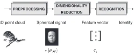
PREPROCESSING DIMENSIONALITY REDUCTION 3D point cloud RECOGNITION (θ,ϕ) i s ci Identity Spherical signal Feature vector

[ ]

. . .

Figure 1: Block diagram of the 3D face recognition system.

tication or human-computer interaction. The face is an easily collectible, univer-sal and non-intrusive biometric [1], which makes it ideal for applications where other biometrics such as fingerprints or iris scanning are not possible.

There has been a considerable progress in the area of two-dimensional face recognition where intensity/color images of human faces are employed. However, these systems are sensitive to illumination, pose variations, occlusions, facial expressions and make-up. On the other hand, recognition systems based on 3D face information have the potential for greater recognition accuracy and are capable of overcoming part of the limitations of 2D face recognition systems [2, 3]. The 3D shape of a face, usually given as a 3D point cloud, depends on its anatomical structure and it is independent of its pose, which can be further corrected by rigid rotations in the 3D space [4].

We consider in this paper the problem of 3D face recognition and we design a fully automatic algorithm based on simultaneous sparse expansions on the sphere. We first propose a preprocessing step that automatically registers the 3D point clouds prior to dimensionality reduction. It selects the facial region and registers all the faces by an accurate automatic two-step algorithm based on an Average Face Model (AFM) and on the Iterative Closest Point (ICP) algorithm [4]. Contrarily to most of the existing algorithms, the proposed registration process does not require any manual intervention. Registered point clouds are then mapped on the 2D sphere where the spherical face functions are created by nearest neighbor interpolation. The spherical representation enables the use of spherical signal processing techniques, which consider the face signals as combinations of basis functions with diverse shape, position and orientation on

the sphere.

The spherical face signals then undergo a dimensionality reduction step that represents each face with a reduced set of discriminant features. We build a dic-tionary of functions on the sphere and we select the discriminant basis functions by simultaneous sparse approximations. The face signals are finally projected onto the resulting reduced subspace, in order to generate feature vectors. We finally implement a recognition step where Linear Discriminant Analysis (LDA) is performed on the subspace representation of the faces. The recognition sys-tem is illustrated on Fig. 1, wheresi(θ, φ) denotes the spherical signalsi as a function of position (θ, φ) on the 2D sphere, andci is a feature vector.

The performance of the 3D face recognition system is evaluated on the FRGC v.1.0 data set. The proposed algorithm outperforms state-of-the-art solutions based on Principal Component Analysis (PCA, [5]) or Linear Discriminant Anal-ysis (LDA) on depth images. Our fully automatic system provides effective classification performance that shows that 3D face recognition with spherical representations certainly represents a promising solution for person identifica-tion.

The paper is organized as follows. We provide an overview of the related work in 3D face recognition in Section II. Section III describes the automatic face registration process that permits to align the 3D points clouds before analysis. The dimensionality reduction step with simultaneous sparse approximations on the sphere is presented in Section IV and experimental results are finally pro-vided in Section V.

2. Related work

3D face recognition has attracted a lot of research efforts in the past few decades due to the advent of new sensing technologies and the high potential of 3D methods for building robust systems with invariance to head pose and illumination variations. We review in this section the most relevant work in 3D face recognition, which can be categorized in methods using point cloud

rep-resentations, depth images, facial surface features or spherical representations respectively. Surveys of the state-of-the-art in 3D face recognition are further provided in [2, 3].

The recognition methods that work directly on 3D point clouds consider the data in their original representation based on spatial and depth information. A priori registration of the point clouds is commonly performed by ICP algorithms [4, 6]. The classification is generally based on the Hausdorff distance that per-mits to measure the similarity between different point clouds [7]. Alternatively, recognition could be performed with “3D eigenfaces” that are constructed di-rectly from the 3D point clouds [8]. The main drawback of the recognition methods based on 3D point clouds however resides in their high computational complexity that is driven by the large size of the data.

Many recognition systems use depth or range images that permit to for-mulate the 3D face recognition as a problem of dimensionality reduction for planar images, where each pixel value represents the distance from the sensor to the facial surface. Principal Component Analysis (PCA) and “Eigenfaces” can be used for dimensionality reduction [9], where the basis vectors are how-ever typically holistic and of global support. PCA can be combined with Linear Discriminant Analysis (LDA) to form “Fisherfaces” with enhanced class separa-bility properties [10]. Alternatively, dimensionality reduction can be performed via variants of non-negative matrix factorization (NMF) algorithms [11, 12, 13] that produce part-based decompositions of the depth images. Part-based de-compositions based on non-negative sparse coding [14] have recently been shown to provide improved recognition performance than NMF methods in face recog-nition [15]. Recent methods have proposed to concentrate dimensionality re-duction around facial landmarks like the nose tip [16] or in multiple carefully chosen regions [17] or to compute geodesic distances among the selected fiducial points [18]. They however require a selection of the fiducial points or areas of interest that is often performed manually and prevents the implementation of fully automatic systems.

idea of recognizing 3D faces using curvature descriptors has been originally in-troduced in [19], where features are chosen to represent both curvature and metric size properties of faces. More recently, level sets of the depth function on range image have been used to define sets of facial curves [20]. They are fur-ther embedded in an appropriately defined shape manifold and compared based on geodesic distances. Facial curve representations provide global information about the whole facial surface, which unfortunately does not permit to take advantage of discriminative local features.

Finally, spherical representations have been used recently for modelling il-lumination variations [21, 22] or both ilil-lumination and pose variations in face images [23]. Spherical representations permit to efficiently represent facial sur-faces and overcome the limitations of other methods towards occlusions and partial views [24]. To the best of our knowledge, the representation of 3D face point clouds as spherical signals for face recognition has however not been inves-tigated yet. We therefore propose to take benefit of the robustness of spherical representations and of spherical signal processing tools to build an effective and automatic 3D face recognition system. We perform dimensionality reduction directly on the sphere, so that the geometry of 3D faces is preserved. The re-duced feature space is extracted by sparse approximations with a dictionary of localized geometric features on the sphere that effectively capture spatially localized and salient 3D face features that are advantageous in the recognition process.

3. Automatic preprocessing of 3D face data

3.1. Automatic face extraction

We propose in this section a fully automatic preprocessing method for prepar-ing and alignprepar-ing 3D face point clouds before feature extraction and recognition. Unlike most of the algorithms in the literature, the preprocessing step does not require any manual intervention, which is an enormous advantage for the de-sign of fully automated face recognition systems. The preprocessing scheme is

(a) Binary matrixA_{(b) After lateral}

thresholding

(c) Profile view (d) After depth thresholding (profile view)

(e) After depth thresholding

(f) After morpho-logical processing Figure 2: Main steps in facial region extraction

based on two main tasks, respectively the extraction of the facial region, and the registration of the 3D face. We present these tasks in more details in the rest of the section.

The main purpose of the face extraction step is to remove irrelevant infor-mation from the 3D point clouds, such as data that correspond to shoulder, or hair for example. The output of a facial scan typically forms a 3D point cloud

{X, Y, Z}, whereX and Y form a uniform Euclidean grid andZ provides the corresponding depth values. The point cloud is also accompanied by a binary matrixA of valid points, which has the same resolution as the grid implied by X×Y. The nonzero pattern of such a sample binary matrix is shown in Fig. 2(a). There is however no guarantee that the points exclusively correspond to

face depth information, and face extraction is therefore necessary to ensure that the feature extraction concentrates on capturing discriminative facial informa-tion.

The first step in face extraction consists in removing data points on the subject’s shoulders. We estimate a vertical projection curve from the point cloud by computing the column sum of the matrix A. Then, we define two lateral thresholds on the left and right inflexion points of the projection curve, and we remove all data points beyond these thresholds, as illustrated in Fig. 2(b). We further remove the data points corresponding to the subject’s chest by thresholding of the histogram of depth values. It removes the data points with large depth values that are typically situated behind the data corresponding to frontal face information, as shown in Figs 2(c) and 2(d). We finally have to remove outlier points that remain in regions disconnected from the main facial area, as shown in Fig. 2(e). We therefore perform morphological image processing on the corresponding binary matrixA, where we keep only the largest region that typically correspond to the facial region, as presented in 2(f).

3.2. Automatic face registration

After extracting the main facial region from the 3D scans, the face signals have to be registered in order to ensure that all have the same pose before the recognition step. The registration typically applies rigid transformations on the 3D faces in order to align them. We propose a two-step approach for automatic registration, where an Average Face Model (AFM) is computed and then used for accurate registration.

First, we randomly pick a training face, and we align all the faces approxi-mately to the sample face using the Iterative Closest Point (ICP) algorithm [4]. Given a model and a query point cloud, ICP computes a rigid transformation, consisting of rotations and translations, by minimizing the sum of square errors between the closest model points and query points. After coarse registration with ICP, the face signals are re-sampled on a uniform 2D grid using nearest neighbor interpolation. It permits to construct an AFM, by computing at each

(a) Depth map −0.6 −0.4−0.2 0 0.2 0.4 0.6 0.8 −1 −0.8 −0.6 −0.4 −0.2 0 0.2 0.4 0.6 0.8 −0.1 0 0.1 0.2 0.3 0.4 0.5 0.6 (b) Point cloud

Figure 3: Average Face Model given as a depth map or a 3D point cloud.

(a) Before (depth map) −0.5 −0.4 −0.3−0.2 −0.100.1 0.2 0.30.4 0.5 −0.8 −0.6 −0.4 −0.2 0 0.2 0.4 0.6 0.8 0.05 0.1 0.150.2 0.25 0.3 0.35 0.4 0.45 (b) Before (point cloud)

(c) After (depth map)

−0.5−0.4 −0.3−0.2 −0.10 0.10.20.3 0.40.5 −0.8 −0.6 −0.4 −0.2 0 0.2 0.4 0.6 0 0.1 0.2 0.3 0.4 0.5 (d) After (point cloud)

Figure 4: Illustration of ellipse cropping on depth maps and equivalent 3D point clouds.

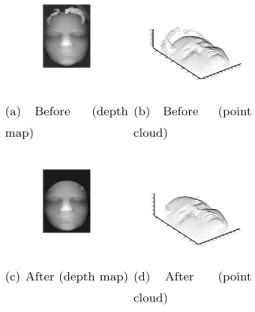
grid point the average depth value among all training faces (see Figure 3) . The AFM is subsequently used as reference in order to define an ellipse that contains the main facial region. Since, the faces are already registered, this ellipse can be used to crop closely all faces in the training set. The ellipse cropping step removes all the irrelevant information that may be left over from the previous preprocessing steps, as shown in Figure 4.

A fine alignment of the faces can now be performed on the signals that have been cleaned from outliers. The accurate alignment is finally obtained by running ICP one more time. The AFM is now used as a reference face model, and all faces signals are registered with respect to the AFM.

4. Recognition with sparse spherical representations

4.1. Simultaneous sparse approximations

Efficient face recognition algorithms usually include a dimensionality reduc-tion step, where high dimensional data are represented in a reduced subspace. We propose to use sparse signal representation methods for dimensionality re-duction. Such methods have demonstrated good performance in 2D face recog-nition [25]. They present the advantage of capturing the main signal charac-teristics in a very small set of meaningful features, which are moreover defined a priori in a dictionary of functions. This presents an interesting advantage compared to classical methods such as PCA, whose feature vectors are data-dependent. In addition, a proper choice of the dictionary permits to build features that capture the geometrical information in the face signal. We give below a brief overview of sparse approximations, and we show later how we use them for dimensionality reduction on the sphere.

Let denote bysi, i= 1, ..., N, a set of functions in the Hilbert spaceH. Let further denote byD={gγ, γ ∈Γ} an overcomplete dictionary of unitL2 norm

functions indexed by γ, which spans the space H. A function si has a sparse representation inDif it can be represented in terms of a linear superposition of small set of basis functions{gγ} ∈ D . In other words, it can be expressed as si = ΦI ici, where ΦI i denotes a matrix whose columns are atoms in DI i ⊂ D that forms the sparse support of the signal si. The vector ci represents the coefficients of the linear approximation ofsi with atoms inDI i.

Finding the sparsest representation of a signal in a redundant dictionaryD

is in general an NP-hard problem. Greedy algorithms like Matching Pursuit [26] have however shown to provide suboptimal yet efficient solutions with a limited computational complexity. It selects iteratively the functions from the dictionary that best matches the signalssi. We have however to ensure that the atoms that form the support of the different signalssi’s are identical, in order to permit to classify them in the feature space. Dimensionality reduction can thus be performed by simultaneous decomposition of all the signalssi, i= 1, ..., N.

Finding the sparse support DI that is common to all the signals {si} can be achieved by the Simultaneous MP (SMP) [27] algorithm, which only induces a small increase of complexity compared to MP on a single signal [25]. In short, SMP greedily selects DI such that all the N functions si are simultaneously approximated in the same basis. It results in the extraction ofK atoms such that all signals are simultaneously represented by linear combinations of them. Each signal can be re-written assi = ΦIci, where ΦI denotes the matrix whose columns are the atoms in the common sparse support DI ⊂ D. Finally, a few iterations are typically sufficient to capture most of the energy of the face signals to be approximated. It has been shown that residual error of the SMP approximation decays exponentially for correlated signals with the same support and additive white noise [27].

4.2. Spherical subspace selection with SMP

We propose to perform the classification of 3D face by dimensionality re-duction on the sphere. We therefore project the 3D point cloud onto the unit sphere S2

, and then we select a subspace that spans functions on S2

. Since faces are typically star-shaped objects, spherical projection preserves the face geometry information, while reducing the classification complexity by map-ping a 3D signal to a 2D spherical signal. Each face, given by a 3D point-cloud {pn} = {(xn, yn, zn)} is, therefore, represented as a spherical function r=s(θ, ϕ) sampled at points {(rn, θn, ϕn)}, which are obtained by transform-ing Euclidean coordinates from the point cloud to spherical coordinates given by (θ, ϕ) that represent the elevation and azimuth angles.

Since we represent 3D faces as square-integrable functions onS2

, denoted as L2

(S2

), we can use the SMP to select a subspace of spherical basis functions as a dimensionality reduction step. We use a spherical dictionary proposed in [28], where the atoms are created by applying local geometric transforms to a gener-ation functiong(θ, ϕ) defined on the sphere. Local transforms include atom mo-tion (τ, ν) (position on the sphere with respect to (θ, ϕ), respectively), rotation ψ, and anisotropic scaling by two scales (α, β) in orthogonal directions. Motion

Figure 5: Gaussian atoms.

and rotation are realized using a rotation inSO(3), which is the rotation group in R3

. Five transform parameters form the atom indexγ = (τ, ν, ψ, α, β)∈Γ, and the redundant dictionary is finally constructed by applying a large set of differentγ’s tog. A detailed explanation of the dictionary construction is given in [28]. An example of the generating function is a 2-D Gaussian function in L2

(S2

), given by:

g(θ, ϕ) = exp(−tan2θ

2). (1)

Function in Eq.(1) represents an isotropic gaussian function, centered at the North Pole. In Figure 5 we show a few sample Gaussian atoms that are obtained by applying different local transforms to the generating function in Eq.(1).

Equipped with the spherical dictionary, we can directly apply SMP to find the common support of the spherical faces, where the inner product between two spherical functionsf =f(θ, ϕ) andg=g(θ, ϕ) is however given by:

hf, gi= Z θ Z ϕ f(θ, ϕ)g(θ, ϕ) sinθdθdϕ. (2) In the following, we refer to this special case of SMP for spherical signals using the dictionary defined on the sphere, assimultaneous spherical matching

pursuit (SSMP).

4.3. Recognition on the sphere

The algorithm for recognition of 3D faces on the sphere is finally illustrated in Figure 6. The first step performs dimensionality reduction, by projecting the spherical signals on the subspace spanned by the selected atoms i.e., span{DI}, as described above. If we denote the set of face signals by S = [s1, . . . , s_n],

DIM REDUCTION SSMP LDA MATCHING Φ

(

)

(

)

Training faces Class label

C~

Figure 6: Block diagram of the recognition process.

set ofKbasis vectorsDI ={gγ1, . . . , gγK} from the dictionaryD, such that all

spherical faces are simultaneously approximated as,

S≈ΦI ·C. (3)

The matrixC∈RK×n _{holds the coefficient vectors (in its columns) and Φ} I = [gγ1, . . . , gγK].

The coefficient vector conveys quite discriminative information about the faces signals. However, the class separability of the coefficient vectors in the reduced space could yet be improved by performing an optional Linear Dis-criminant Analysis (LDA) step before matching. LDA exploits the class labels information of the training samples in order to enhance the discriminant prop-erties of the coefficient vectors. It introduces supervision in the recognition process and permits to build a new set of coefficient vectors ˜C = CW where the weightsW are chosen to optimize the ratio of between-class variance and within-class variance for training data [10].

Finally, the matching is performed by comparing the coefficient vectorsC, which represent the lower dimensional data samples. The recognition is per-formed by nearest neighbor classification. We iteratively compute the coeffi-cientsctof the test face signal ston the sub-dictionary DI. The classification is then performed by computing theL1distance betweenc_t and any coefficient

vectorci corresponding to the training signals d(ct, ci) =

K

X

j=1

|ct(j)−ci(j)|. (4)

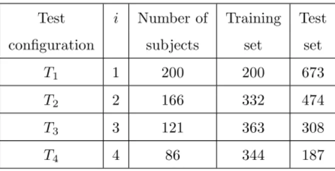
Test i Number of Training Test

configuration subjects set set

T1 1 200 200 673

T2 2 166 332 474

T3 3 121 363 308

T4 4 86 344 187

Table 1: Test configurations and their characteristics.

to the smallest distance d(ct, ci) between the coefficients vectors. The same classification method is used for coefficients ˜C modified by LDA. The choice of the L1 distance metric is mostly empiric as it leads to superior classification

performance compared to other metrics.

5. Experimental results

5.1. Experimental setup

In this section, we evaluate the performance of the proposed algorithms in both recognition and verification scenarios. We compare our algorithms with PCA and LDA on depth images that have undergone the same preprocessing step as the data used in the SSMP algorithm. PCA and LDA are well known methods that represent state-of-the-art technologies for 3D recognition.

For our evaluation, we use the UND (University of Notre Dame) Biometric database [29, 30], also known as FRGC v.1.0 database. It contains 953 facial images of 277 subjects, where each subject has between one and eight scans. Each facial scan is provided in the form of a 3D point-cloud, along with a corresponding binary matrix of valid points. The number of vertices in a point-cloud typically varies between 30.000 and 40.000.

We defined several test configurations for our experimental evaluation. Each configuration is characterized by the number of samples per subject that form the training set. For each configurationTi, we keep only the subjects from the

database that have at least i+ 1 samples, and we use i training samples per class (randomly chosen), while assigning the rest to the test set. The subjects that have only one facial scan can not be used in the recognition tests. Table 1 summarizes the test configurations and their main characteristics.

SSMP implementation. For the dictionary construction in SSMP-based

meth-ods, we have used the 2D Gaussian on the sphere (1) as the generating function. The atom indexesγ that define the dictionary, have to take discrete values in practice. We use here a discretization of the dictionary as in [28], mostly built on empirical choices for atom parameter values. The position parameters,τand νare uniformly distributed on the interval [0, π], and [−π, π), respectively, with equal resolution of 128 points. The rotation parameterψ is uniformly sampled on the interval [−π, π), with the same resolution as τ and ν. This choice is mostly due to the use of fast computation of correlation on SO(3) for the full atom search within the SSMP algorithm. In particular, we used the

Spharmon-icKit library1

, which is part of the YAW toolbox2

. Finally, scaling parameters are distributed in a logarithmic manner, from 1 to half of the resolution of τ andν, with a granularity of one third of octave. The largest atom covers half of the sphere.

The use of fast computation of correlation on the SO(3) group requires the spherical data to be sampled on an equiangular (θ, ϕ) grid, defined as:

G={(θi, ϕj), θi = (2i+ 1)π 2Nθ , andϕj = j2π Nϕ }. (5)

where: i = 0, ..., Nθ−1 andj = 0, ...Nϕ−1. Since 3D face point clouds are projected as scattered data on the sphere, an interpolation step is necessary. For its simplicity we use k-nearest neighbor interpolation, where the value on each spherical grid point (θi, ϕj) is computed as an average of its k nearest neighbors. We have used k = 4 and a resolution of Nθ = 128, Nϕ = 128. Note finally that, for the sake of computational ease, dimensionality reduction

1_{http://www.cs.dartmouth.edu/∼geelong/sphere/} 2

with SSMP is performed off-line, using only one training face per subject. The resulting subspace is then used for projecting both training and test samples.

Virtual faces. The size of the training set is important in determining the

clas-sification performance. We propose to enrich the training set withvirtual faces

(see e.g., [31] and references therein). These are faces that are artificially gen-erated by slight variations of the original training faces. They are given the corresponding class labels of the training face they originate from, and they are treated as training samples. The use of virtual faces is motivated by two main reasons: (i) they compensate for small registration errors (recall that our registration process is fully automatic and it is expected to contain a few reg-istration errors) and (ii) by augmenting the training set, they may contribute to the performance of sample-based methods (e.g., LDA) that can benefit from large sample sets. Note that the virtual faces do not introduce any new infor-mation to the training set, since they are synthetically generated by the original training faces. For computational convenience, we construct them by one or two pixel translations in the spherical domain. Note finally that virtual faces are used only in the SSMP+LDA method.

5.2. Recognition results

We present recognition results of our methods and we compare them with PCA and LDA on depth images. For the sake of completeness, we also report the classification performances of the Euclidean distance (EUC) between depth images, and Mean Square Error (MSE) between spherical functions. For the two latter methods, each test face is recognized as the closest neighbor in the training set. In SMMP+LDA (resp. PCA+LDA), the number of dimensions used in LDA is set to the minimum between the number of features in SSMP (resp. PCA) and c−1, wherec is the number of classes (subjects). Virtual faces are used in the SSMP+LDA method in configurationsT1,T2 andT3only,

since they correspond to small training sets. In these cases, each training face is used to generate 8 virtual faces.

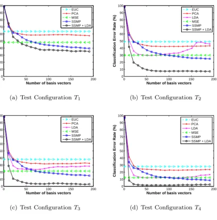
0 50 100 150 200 0 10 20 30 40 50 60 70 80 90 100

Number of basis vectors

Classification Error Rate (%)

EUC PCA MSE SSMP SSMP + LDA

(a) Test ConfigurationT1

0 50 100 150 200 0 10 20 30 40 50 60 70 80 90 100

Number of basis vectors

Classification Error Rate (%)

EUC PCA LDA MSE SSMP SSMP + LDA (b) Test ConfigurationT2 0 50 100 150 200 0 10 20 30 40 50 60 70 80 90 100

Number of basis vectors

Classification Error Rate (%)

EUC PCA LDA MSE SSMP SSMP + LDA (c) Test ConfigurationT3 0 50 100 150 200 0 10 20 30 40 50 60 70 80 90 100

Number of basis vectors

Classification Error Rate (%)

EUC PCA LDA MSE SSMP SSMP + LDA (d) Test ConfigurationT4

Figure 7: Rank-1 recognition results: average classification error rate versus the dimension of the subspace.

We start with rank-1 recognition, which refers to the scenario where a class prediction is considered to be a hit when the label of the closest neighbor is the correct one. Then, we will discuss the generic rank-k scenario, where the prediction is a hit when the correct label is included in the labels of the closest kneighbors.

Rank-1 recognition. All tests are performed 10 times, by splitting randomly the

samples into the training and the test sets. Figure 7 shows the classification error rate for all configurations, averaged over the 10 random experiments. No-tice the remarkable improvement introduced by the employment of spherical functions for facial representation. This is evident from the fact that the recog-nition performance of nearest neighbor classification with Mean Square Error

T1 T2 T3 T4

PCA 45,17 60,97 74,35 82,89

PCA + LDA - 74,89 80,52 93,58

SSMP 62,85 77,22 87,01 94,12

SSMP + LDA 67,61 94,73 98,70 100

Table 2: Best rank-1 recognition rates (%) reached by each method in experiment 5.2.

0 20 40 60 80 100 40 50 60 70 80 90 100 Rank Recognition rate (%) PCA SSMP SSMP + LDA

(a) Test ConfigurationT1

0 20 40 60 80 100 40 50 60 70 80 90 100 Rank

Recognition rate (%) PCA

LDA SSMP SSMP + LDA

(b) Test ConfigurationT2

Figure 8: Rank-k_{recognition results in terms of CMC curves.}

(MSE) between spherical signals, outperforms that of Euclidean distances be-tween depth images (EUC). This provides also the main motivation for working on the sphere. Based on this observation, it seems reasonable that our SSMP al-gorithm outperforms PCA in all configurations. Notice finally that SSMP+LDA is the best performer. In T2, SSMP reaches recognition performance of 77,22%, while SSMP+LDA reaches 94,73%. The latter goes to the maximum 100% in T4, even in the absence of virtual faces. Table 2 shows the highest recognition rates achieved by each method in all configurations.

Rank-krecognition. We report rank-krecognition performances in terms of

cu-mulative match characteristic (CMC) curves. A CMC curve simply illustrates the fluctuation of the recognition rate versus the rank k. Figure 8 shows the obtained CMC curves forT1 andT2 that represent the most interesting cases,

since T3 and T4 correspond to very good performances for all methods. The CMC curves in this figure are averages over 10 random tests, where the best number of dimensions for each algorithm is used (obtained from the previous rank-1 recognition experiments). As expected, notice again that SSMP is su-perior to PCA, and LDA introduces in both methods a significant performance boost. 5.3. Verification results 0 0.2 0.4 0.6 0.8 1 0 0.2 0.4 0.6 0.8 1

False Positive Rate

True Positive Rate

SSMP SSMP+LDA PCA

(a) Test ConfigurationT1

0 0.2 0.4 0.6 0.8 1 0 0.2 0.4 0.6 0.8 1

False Positive Rate

True Positive Rate

SSMP + LDA SSMP PCA LDA (b) Test ConfigurationT2 0 0.2 0.4 0.6 0.8 1 0 0.2 0.4 0.6 0.8 1

False Positive Rate

True Positive Rate

SSMP SSMP+LDA PCA LDA (c) Test ConfigurationT3 0 0.2 0.4 0.6 0.8 1 0 0.2 0.4 0.6 0.8 1

False Positive Rate

True Positive Rate

SSMP SSMP+LDA PCA LDA

(d) Test ConfigurationT4

Figure 9: Verification performance in terms of ROC curves.

We compare now all the above methods in the verification scenario, where the test subject claims an identity and the system has to either accept or reject this claim. If the identity is the correct one, then the test subject is called aclient; otherwise, it is called an impostor. In systems that output a confidence score

about the test subject, a hard decision (i.e., accept or reject) is typically reached according to a threshold value. We report the verification performances in terms of receiver operating characteristic (ROC) curves, which show the fluctuation of the true positive rate (TPR) versus the false positive rate (FPR) across all values of the threshold. For the computation of the ROC curve we consider every possible pair of subject and claimed identity.

In our experimental setup, we use the dimensions that yields the best perfor-mance, which corresponds to 200 atoms in SSMP and 100 dimensions in PCA. The number of LDA dimensions in both SSMP+LDA and PCA+LDA is set with the same rule as in the recognition experiments (i.e., using the minimum between the number of PCA/SSMP features andc−1). Also, in SSMP+LDA we use virtual faces only for configurations T1 and T2. Figure 9 shows the average ROC curves over 10 random experiments for all configurations. Similar conclusions can be drawn here as well. Unsurprisingly, observe again that SSMP consistently outperforms PCA in all configurations and SSMP+LDA is the best performer.

5.4. Discussion

It is worth noting that supervised versions of SSMP could be also used [25]. The idea would be then to select the atoms from the dictionary according to discriminative criteria. However, in the proposed scheme the supervision information is already taken into account in the LDA postprocessing step, and prior experience has shown that this suffices, when predefined dictionaries are used.

Note also that the importance of each region of the face in terms of recogni-tion performance is certainly not uniform [17]. Although the selecrecogni-tion of such regions is typically performed manually and it maybe sensitive to the testing conditions, one possible approach to take advantage of this observation could be to group the features selected by SSMP into regions by clustering on the sphere, do a classification per region and then fuse the results (e.g., by majority voting). Such an approach however requires a sufficient number of atoms in each area,

and the performance of such a region-based classifier has not been convincing. Note finally that the proposed dimensionality reduction scheme is generic and simple extensions could be proposed to make the classification more sen-sitive to some specific areas. For example, the SSMP scheme can easily be adapted to give priorities to regions of high interest such as the nose or the eyes. Such a prioritization can be achieved by giving proper weights to atoms located in different areas, in order to force the dimensionality reduction step to select features in areas that are expected to be more discriminative. This however goes along the lines of supervised versions of SSMP mentioned above with the main difference that discriminative capability in this case is mostly defined in a region-based way.

6. Conclusions

We have proposed a methodology for 3D face recognition based on spherical sparse representations. First, we introduced a fully automatic process for ex-traction, preprocessing and registration of facial information in 3D point clouds. Next, we proposed to convert faces from point clouds to spherical signals. Sparse spherical representation of faces allows for effective dimensionality reduction through simultaneous sparse approximations. The dimensionality reduction step preserves the geometry information, which in turn leads to high performance matching in the reduced space. We provide ample experimental evidence that indicates the advantages of the proposed approach over state-of-the-art methods working on depth images.

7. Acknowledgements

The authors would like to thank Prof. Patrick Flynn for sharing with us the UND Biometrics database.

References

[1] A. Jain, L. Hong and S. Pankati. “Biometric Identification”.Communications of

the ACM, vol. 43, no. 2, pp. 90-98. Feb. 2000.

[2] K.W. Bowyer, K. Chang and P. Flynn. “A survey of approaches and challenges

in 3D and multi-modal 3D+2D face recognition”. Computer Vision and Image

Understanding, vol. 101(1), pp. 1-15, Jan. 2006.

[3] L. Akarun, B. Gokberk and A.A. Salah. “3D Face recognition for biometric

ap-plications”.Proc. European Signal Processing Conference, Antalaya 2005.

[4] P. Besl and N. McKay. “A method for registration of 3D shapes”. IEEE Trans.

on Pattern Analysis and Machine Intelligence, vol. 14, pp. 239-256. 1992.

[5] I.T .Jolliffe.Pricipal Component Analysis. Springer Verlag, New york, 1986.

[6] B. G¨okberk, M.O. Irfano˘glu and L. Akarun. “3D shpae-based face representation

and feature extraction for face recognition”. Image and Vision Computing, vol.

24, pp. 857-869. 2006.

[7] B. Achermann and H. Bunke. “Classifying range images of human faces with

Hausdorff distance”.15-th International Conference on Pattern Recognition, pp.

809-813, Sept. 2000.

[8] C. Xu, Y. Wang, T. Tan and L. Quan. “A new attempt to face recognition using

3D Eigenfaces”. Proceedings of the Asian Conference on Computer Vision. (2)

884-889. 2004.

[9] M.A. Turk and A.P. Pentland. “Face recognition using Eigenfaces” . Vision and Modeling Group, The Media Laboratory Massachusetts Institute of Technology. 1996.

[10] P.N. Belhumeur, J.P. Hespanha and D.J. Kriegman. “Eigenfaces vs. Fisherfaces:

recognition using class specific linear projection”IEEE Trans. on Pattern

Anal-ysis and Machine Intelligence., vol. 19, no. 7, July 1997.

[11] D.D. Lee and H.S. Seung.“Algorithms for non-negative matrix factorization”.

Advances in Neural Information Processing Systems (NIPS), vol. 13, pp.

[12] P. Paatero and U. Tapper. “Positive matrix factorization: A non-negative factor

model with optimal utilization of error estimates of data values”.Environmetrics,

vol. 5, pp. 11-126. 1994.

[13] P.O. Hoyer, “Non-negative matrix factorization with sparseness constraits”.

Jour-nal of Machine Learning Research, vol. 5, pp. 1457-1469, 2004.

[14] P. O. Hoyer, “Non-negative sparse coding”, IEEE Workshop on Neural Networks for Signal Processing, pp. 557-565, 2002.

[15] B.J. Shastri and M.D. Levine. “Face recognition using localized features based

on non-negative sparse coding”. Machine Vision and Applications. vol. 18, pp.

107-122, 2007.

[16] S. Jahanbin, H. Choi, A.C. Bovik and K.R. Castleman “Three dimensional face

recognition using wavelet decomposition of range images”International

Confer-ence on Image Processing, pp.145-148, Sep. 2007.

[17] K. Wong, W. Lin, Y. Hu and N. Boston, “Optimal linear combination of facial

regions for improving identification performance”.IEEE Trans. on Systems, Man,

and Cybernetics - Part B: Cybernetics, vol. 37, no. 5, Oct. 2007.

[18] S. Gupta, J.K. Aggarwal, M.K. Markey and A.C. Bovik, “3D face recognition founded on the structural diversity of human faces”, IEEE Conf. on Comp. Vis. and Patt. Rec. (CVPR), June 2007.

[19] G. Gordon. “Face recognition based on depth and curvature features”.SPIE Proc.

Geometric methods in Computer Vision, vol. 1570, pp. 234-247, 1991.

[20] C. Samir, A. Srivastava and M. Daoudi. “Three-dimensional face recognition

using shapes of facial curves” IEEE Trans. on Pattern Analysis and Machine

Intelligence, vol. 28, no. 11, Nov. 2006.

[21] H. Wang, H. Wei and Y. Wang, “Face representation under different illumination

conditions”.IEEE Int. Conf. on Multimedia & Expo (ICME) pp.285-288, 2003.

[22] R. Ramamoorthi. “Analytic PCA construction for theoretical analysis of lighting

variability in images of a Lambertian object”.IEEE Trans. on Pattern Analysis

[23] Z. Yue, W. Zhao and R. Chellappa. “Pose-encoded spherical harmonics for face

recognition and synthesis using a single image”.EURASIP Journal on Advances

in Signal Processing. 2008.

[24] M. Hebert, K. Ikeuchi and H. Delingette. “A spherical representation for

recogni-tion of free-form surfaces”.IEEE Transactions on Pattern Analysis and Machine

Intelligence. vol.17, no.7, July 1995.

[25] E. Kokioppoulou and P. Frossard. “Semantic coding by supervised dimensionality

reduction”IEEE Transactions om Multimedia, vol. 10, no. 5, pp. 806-818, August

2008.

[26] S.G. Mallat and Z. Zhang. “Matching pursuit with time-frequency dictionaries”,

IEEE Trans. on Signal Processing, vol. 41, no. 12, pp. 3397-3415, Dec. 1993.

[27] J. Tropp, A. Gilbert, and M. Strauss. “Algorithms for simultaneous sparse

ap-proximation. Part I: Greedy pursuit”, Signal Processing, special issue “Sparse

approximations in signal and image processing”, vol. 46, pp. 572-588, April 2006.

[28] I. Tosic, P. Frossard and P. Vandergheynst. “Progressive coding of 3D objects

based on overcomplete decompositions”IEEE Transactions on Circuits and

Sys-tems for Video Technology, vol. 16, no. 11, pp. 1338-1349, Nov. 2006.

[29] P. J. Flynn, K. W. Bowyer, and P. J. Phillips, “Assessment of time dependency

in face recognition: An initial study”,Audio and Video-Based Biometric Person

Authentication, pp.44-51, 2003.

[30] X. Chen, P. J. Flynn, and K. W. Bowyer, “Visible-light and infrared face

recogni-tion”, ACM Workshop on Multimodal User Authentication, pp.48-55, December

2003.

[31] D. DeCoste and M.C. Burl, “Distortion-invariant recognition via jittered queries”,