Wavelet Neural Network Based Very Short-term Load Forecasting and Prediction Interval Estimation

University of Connecticut

OpenCommons@UConn

Doctoral Dissertations University of Connecticut Graduate School

8-20-2013

Wavelet Neural Network Based Very Short-term

Load Forecasting and Prediction Interval

Estimation

University of Connecticut - Storrs, [email protected]

Follow this and additional works at:https://opencommons.uconn.edu/dissertations

Recommended Citation

Guan, Che, "Wavelet Neural Network Based Very Short-term Load Forecasting and Prediction Interval Estimation" (2013).Doctoral Dissertations. 172.

Wavelet Neural Network Based Very Short-term

Load Forecasting and Prediction Interval

Estimation

Che Guan, Ph.D.

University of Connecticut, 2013

Very short-term load forecasting predicts the loads in electrical power network one or

several hours into the future in steps of a few minutes (e.g., five minutes) in a moving

window manner based on online data collected every few seconds (e.g., four seconds). In

order to quantify forecasting accuracy in real-time, the forecasting process should also

estimate good prediction intervals online. Accurate forecasting with prediction intervals is

important for resource dispatch and area generation control, and helps power market

participants make prudent decisions. It is, however, difficult in view of the noisy data

collection process with possible malfunctioning of data gathering devices, the different

characteristics of load frequency components, and the accurate derivation and evaluation for

prediction interval estimation in real-time.

This thesis presents a method of multilevel wavelet neural networks with data

pre-filtering. The key idea is to use a spike filtering technique to detect spikes in load and correct

them without altering the normal load. Wavelet decomposition is then used to decompose

the load into multiple components at different frequencies, separate neural networks are

then combined to form the final forecast. To perform moving forecast over an hour, twelve

dedicated structures are used based on testing results.

Because wavelet neural networks are based on back propagation without estimating

prediction intervals, the method is extended by using hybrid Kalman filters to produce

forecasting with prediction interval estimates online. Based on data analysis, a neural

network trained by an extended Kalman filter is used for the low-low frequency component

to capture the near-linear relationship between the input load component and the output

measurement, while neural networks trained by unscented Kalman filters are used for

low-high and low-high frequency components to capture their nonlinear relationships. The overall

variance estimate is then derived and evaluated for prediction interval estimation.

Testing results demonstrate the effects of data pre-filtering, the accuracy of wavelet

neural networks, the effectiveness of hybrid Kalman filters for capturing different features of

load components, and the accuracy of derived prediction interval estimates, based on a data

Wavelet Neural Network Based Very Short-term

Load Forecasting and Prediction Interval

Estimation

Che Guan

B.S., Changchun University of Science and Technology, Changchun, China, 2004

M.S., Chinese Academy of Sciences, Beijing, China, 2007

M.S., University of Connecticut, Storrs, USA, 2011

A Dissertation

Submitted in Partial Fulfillment of the

Requirements for the Degree of

Doctor of Philosophy

At the

University of Connecticut

2013

Copyright by

Che Guan

APPROVAL PAGE

Doctor of Philosophy Dissertation

Wavelet Neural Network Based Very Short-term

Load Forecasting and Prediction Interval

Estimation

Presented by

Che Guan, B.S., M.S.

Major Advisor:

Peter B. Luh

Associate Advisor:

Yaakov Bar-Shalom

Associate Advisor:

Laurent D. Michel

University of Connecticut

2013

Acknowledgements

It has been a great pleasure to spend six years as a graduate student at UConn. Here I

met many wonderful scientists and friends who play important roles on me to become a

researcher, and have contributed significantly to the work in my dissertation.

I would like to express my sincerest gratitude to my advisor, Professor Peter B. Luh,

for his continuous guidance, encouragement, patience, and opportunities given to me to

practice and grow up. All the works could not be accomplished without his persistent

supervision, and I am appreciated very much. I am also very grateful to Dr. Ying Chen. As

a graduated member from the lab as well as a best friend, she has been selflessly sharing her

precious experiences and helping me overcome many difficulties on the way to the Ph.D.

target. It is really a fortunate to work with her.

I would like to thank my co-advisors Professor Yaakov Bar-Shalom and Professor

Laurent Michel for their supervision and help on my research. I am also thankful to

Professor Zhiyi Chi for his consistent help on my research, and Professor Shengli Zhou for

his review of this dissertation. I would also like to thank Dr. Kwok Cheung at the Alstom

Grid, and Peter B. Friedland who was at the ISO New England for their continuous supports

on my research, as well as Mr. Matthew A. Coolbeth, Mr. Yuting Wang, and Mr. Stephen

Corbo, for their continuous supports on my research. I am also thankful to Miss Fang Chen,

Dr. Yi Yang, Dr. Tian Mi, Dr. Shuo Zhang, Dr. Ying Wang, etc., for their information and

consistent help on my dissertation.

I would like to thank all the past and present lab members at Manufacturing Systems

Dr. Jin Sun, Dr. Guoyu Tu, Dr. Mingyang Li, Mr. William E. Blankson, Mr. Abhinaya Joshi,

Mr. Majid Chauhdry, Mr. Peng Wang, Mrs. Bingjie Zhang, Miss Congcong Wang, Mr. Xu

Han, Mr. Liangliang Sun, Mr. Yige Zhao, Mrs. Weihua Wang, Mrs. Bing Yan, Mr. Mikhail

Bragin, Mrs. Yu Chen, Mr. Ying Yan, Mr. Yaowen Yu, Miss Xiaorong Sun, Mr. Weiji Han,

Mr. Biao Sun, Mr. Christian Wilkie, etc. It was a great pleasure to meet you, and I've

enjoyed working with you and take tremendous pride in what we've been able to accomplish.

The six-year life in the lab leaves with me many fond memories and valued relationships.

I would like to express my sincere appreciation for my colleagues at the Dun and

Bradstreet, especially for: Dr. Nipa Basu and the whole worldwide predictive analytic team’s

consistent supports, and Dr. Anthony Scriffignano for his encouragement, help, and support

on my oral defense of dissertation.

Finally I would like to thank my family, especially for my parents Mr. Yongjun Guan

and Mrs. Jun Sun. Whenever, wherever, and whatever I am in need, you are always there.

Without your support, I would have not been able to accomplish as much as I have.

Table of Contents

2. Very Short-term Load Forecasting: Wavelet Neural Networks with Data Pre-filtering ... 7

2.1 Introduction ... 7

2.2 Literature Review ... 9

2.3 Data Pre-filtering ... 13

2.3.1 Micro Spike Filtering... 14

2.3.2 Macro Spike Filtering ... 16

2.4 Wavelet Neural Networks ... 17

2.4.1 Load Property Analysis... 18

2.4.2 Filter Bank in Wavelet Transform ... 20

2.4.3 Neural Networks ... 24

2.4.4 Moving Forecasts... 27

2.5 Numerical Test Results ... 27

2.6 Conclusion... 43

3. Hybrid Kalman Filters for Very Short-term Load Forecasting and Prediction Interval Estimation ... 45

3.1 Introduction ... 45

3.2 Literature Review ... 49

3.2.1 Prediction Interval Estimation ... 49

3.2.2 Wavelet Neural Networks... 51

3.4 Wavelet Neural Networks Trained by Hybrid Kalman Filters... 52

3.3.1 EKFNN for the Low-Low Load Component... 55

3.3.2 UKFNN for the Low-High and High Load Components ... 58

3.4 Prediction Iinterval Estimation and Evaluation ... 61

3.4.1 Prediction Interval Estimation ... 62

3.4.2 Evaluation of Prediction Interval Estimates ... 64

3.5 Numerical Testing Results ... 65

3.6 Conclusion ... 81

4. Summary and Future Research ... 83

4.1 Summary ... 83

4.2 Future Research Directions... 84

List of Figures

FIGURE 2-1. BEFORE (TOP) AND AFTER (BOTTOM) MICRO AND MACRO SPIKE FILTERING BASED ON TWO DAYS OF CONTINUOUS ISO-NE LOAD DATA AT THE FOUR-SECOND RESOLUTION16 FIGURE 2-2. BEFORE (TOP) AND AFTER (BOTTOM) MACRO SPIKE FILTERING AT THE FIVE

-MINUTE RESOLUTION... 17

FIGURE 2-3. POWER SPECTRUM DENSITY FOR FIVE-MINUTE LOAD DATA (JANUARY 1ST,2007 TO JUNE 30TH,2008) ... 19

FIGURE 2-4. AMPLITUDE SPECTRUM FOR FIVE-MINUTE LOAD DATA... 20

FIGURE 2-5. THREE-CHANNEL FILTER BANK... 21

FIGURE 2-6. STRUCTURE OF WAVELET NEURAL NETWORKS... 24

FIGURE 2-7.A. AMPLITUDE SPECTRUM FOR NORMALIZED LOW-LOW FREQUENCY BEFORE APPLYING RI; FIGURE 2-7.B. AMPLITUDE SPECTRUM FOR NORMALIZED LOW-LOW FREQUENCY AFTER APPLYING RI ... 26

FIGURE 2-8. BOX PLOTS FOR FORECASTING ERRORS FOR 5 TO 60 MINUTE OUTS... 38

FIGURE 3-1. SCHEMATIC OF THE WAVELET NEURAL NETWORKS (WNN) ... 51

FIGURE 3-2. SCATTER PLOTS OF 60-MIN-AHEAD PREDICTIONS AND RESIDUALS FOR INDIVIDUAL LL,LH, AND H LOAD COMPONENTS (BASED ON 1000 PAIR DATA FOR INDIVIDUAL PLOTS) ... 53

FIGURE 3-3. SCHEMATIC OF WAVELET NEURAL NETWORKS TRAINED BY HYBRID KALMAN FILTERS (WNNHKF) ... 54

FIGURE 3-4. SCHEMATIC OF THE PREDICTION INTERVAL ESTIMATION... 62

FIGURE 3-5. QUANTILE-QUANTILE PLOT OF THE 5 MIN-AHEAD FORECASTING ERRORS VERSUS THE STANDARD NORMAL... 73

FIGURE 3-6. THE AMOUNT OF ESDS AS A FUNCTION OF COVERAGE RATES RANGING FROM 10% TO 90% FOR EACH LOOK-AHEAD TIME WHEN COMPARED WITH THE AMOUNT OF SIGMAS UNDER THE STANDARD GAUSSIAN... 76

FIGURE 3-7. THE AMOUNT OF ESDS AS A FUNCTION OF COVERAGE RATES RANGING FROM 91% TO 99% FOR EACH LOOK-AHEAD TIME WHEN COMPARED WITH THE AMOUNT OF SIGMAS UNDER THE STANDARD GAUSSIAN... 77

List of Tables

TABLE 2-1. MAES (MW) FOR MULTIPLE WNNS... 31

TABLE 2-2. MAPES (%),MAES (MW), AND SDS (MW) FOR MULTIPLE WNNS IN MOVING FORECASTS WITH AND WITHOUT SPIKE FILTERING METHODS... 32

TABLE 2-3. MAES (MW) AND SDS (MW) FOR SPIKE FILTERING METHODS WITH DIFFERENT M VALUES... 33

TABLE 2-4. MAES (MW) AND SDS (MW) FOR WNN1 WITH DIFFERENT DECOMPOSITION LEVELS... 34

TABLE 2-5. MAES (MW) FOR WNN1 WITH DIFFERENT DAUBECHIES WAVELETS... 35

TABLE 2-6. MAES (MW) FOR THE WNN1 WITH DIFFERENT PADDING STRATEGIES... 35

TABLE 2-7. MAES (MW) FOR WNN1 WITH DIFFERENT TIME INDICES... 36

TABLE 2-8. MASES,MAPES (%),MAES (MW), AND SDS (MW) FOR OUR METHOD... 37

TABLE 2-9. MAPES (%) AND MAES (MW) COMPARING OUR METHOD’ RESULTS TO ISO-NE’S RESULTS... 40

TABLE 2-10. MEANS AND STANDARD DEVIATIONS FOR MAPES (%),MAES (MW), AND SDS (MW) FROM MONTE CARLO SIMULATIONS WITH A RANDOM WEIGHT INITIALIZATION (WITH N=20SIMULATIONS) ... 42

TABLE 2-11. MEANS AND STANDARD DEVIATIONS FOR MAPES (%),MAES (MW), AND SDS (MW) FROM MONTE CARLO SIMULATIONS WITH RANDOM RE-SAMPLING STEPS (WITH N=20SIMULATIONS) ... 43

TABLE 3-1. NO. OF HIDDEN NEURONS,AVERAGED MAES, AND AVERAGED SDS COMPARING THE RESULTS OF WNNHKF TO THE RESULTS OF PERSISTENCE,LINEAR AR,SINGLE NN, AND WNN ... 67

TABLE 3-2.MAPES (%) AND SDS (MW) FOR DIFFERENT COMBINATIONS OF NNS TRAINED BY KALMAN FILTER(S) FOR INDIVIDUAL LOAD COMPONENTS... 68

TABLE 3-3.MAPES (%),MAES (MW),SDS (MW),ESDS (MW), AND ONE SIGMA COVERAGE (%) FOR WNNHKFMETHOD (BASED ON VALIDATION DATA SET) ... 70

TABLE 3-4.MAPES (%),MAES (MW),SDS (MW),ESDS (MW), AND ONE SIGMA COVERAGE (%) FOR WNNHKFMETHOD (BASED ON TEST DATA SET) ... 71

TABLE 3-5. TOTAL PROBABILITY MASS (%) OF TAILS OF ERROR REMOVED TO MAKE KOLMOGOROV–SMIRNOV TEST INSIGNIFICANT (P>0.1) ... 73

TABLE 3-6.AMOUNT OF ESD TO ACHIEVE ALMOST THE SAME COVERAGE RATES... 74

TABLE 3-7. ACTUAL COVERAGE RATES (%) OF EMPIRICAL QUANTILE-BASED PIS FOR DIFFERENT NOMINAL COVERAGE RATES... 78

TABLE 3-8. WIDTHS (MW) OF EMPIRICAL QUANTILE-BASED PIS FOR DIFFERENT NOMINAL COVERAGE RATES AS SHOWN IN TABLE 3-7 ... 79

TABLE 3-9. WIDTHS (MW) OF STANDARD-DEVIATION-BASED PIS ACHIEVING THE SAME ACTUAL COVERAGE RATES AS SHOWN IN TABLE 3-7... 79

TABLE 3-10. MAPES (%) COMPARING THE RESULTS OF WNNHKF TO THE RESULTS OF PERSISTENCE,LINEAR ARMODEL,ISO-NE’S METHOD, AND WNN ... 81

1

1.

Introduction

1.1

Research Motivation

Very short-term load forecasting (VSTLF) predicts the loads in electrical power

network one or several hours into the future in steps of a few minutes (e.g., five minutes) in a

moving window manner based on online data collected every few seconds (e.g., four

seconds). To quantify forecasting accuracy in real-time, the forecasting process should also

estimate accurate prediction intervals (PI) online. Accurate VSTLF with good PIs is

important for resource dispatch and area generation control, and helps power market

participants make prudent decisions. Based on data analysis, load time series have multiple

frequency components, and each may have its unique pattern, such as monthly, weekly, and

hourly patterns. Effective VSTLF, however, is difficult in view of the noisy data collection

process with possible malfunctioning of data gathering devices, different characteristics of

load components, and the accurate derivation for estimating prediction intervals online.

1.2

Dissertation Outline

The research of this dissertation is to advance real-time load forecasting methods in

electrical power network. The study is an extension of the previous method for short-term

load forecasting (STLF) which predicts the loads of tomorrow in hourly steps based on the

single-level wavelet decomposition and neural networks trained through using a data set from

ISO New England (Chen et al., 2010). The method presented a way for handling load

2

the ones of VSTLF because short-term load data have fewer patterns than very short-term

load data to be analyzed. Also, spikes were not considered because they had been removed

by ISO New England before STLF was performed, whereas removing spikes is a critical

issue for VSTLF.

In Chapter 2, wavelet neural networks (WNN) with data pre-filtering will be developed

to forecast the loads one hour into the future in five-minute steps in a moving window

manner. To effectively remove spikes, it is observed that spikes may have different

magnitudes and widths. Thus, they are classified into micro and macro spikes at either

four-second or five-minute resolutions. Micro and macro filtering techniques will be developed to

effectively detect and filter them out. To accurately capture load features, the wavelet

technique will be used to decompose the loads into multiple frequency components. Each

component is then appropriately transformed, normalized, and fed with time and date indices

to a neural network, so that the features of individual components are properly captured.

Forecasts from individual neural networks are then transformed back and combined to form

the final forecasts. To perform moving forecasts, twelve dedicated wavelet neural networks

will be used based on preliminary simulation results.

In Chapter 3, the method of wavelet neural networks will be further improved to

provide prediction intervals. By replacing the first-order back propagation algorithm with

second-order Kalman type algorithms, dynamic covariance can be produced for prediction

interval estimation. The method of wavelet neural networks trained by hybrid Kalman filters

(WNNHK) will be developed. It forecasts the loads one hour into the future in 5-min steps in

a moving window manner with associated PI estimates online. After a data analysis, it is

3

the low frequency load input and its measurement, whereas the Low-High (LH) and High (H)

frequency components have the nonlinear relations. To capture the near-linear relationship

between the input and measurement for the LL component, the extended Kalman filter is

used to train a neural network (EKFNN) because the extended Kalman filter is derived by

linearizing the system and is good for near-linear systems. To capture highly nonlinear

relationships for the LH and H components, the unscented Kalman filter is used to train

neural networks (UKFNN) because the unscented Kalman filter is good for highly nonlinear

systems. To accurately estimate prediction intervals online, the overall variance estimate will

be calculated by summing up the three orthogonal variance estimates from H, LH, and LL

frequency neural networks. The estimates for H and LH components are directly obtained.

The estimate for the LL component is further derived because the relative increment, a

nonlinear transformation, is applied to the LL component. The relative increment is used to

make the series stationary so that the transformed series can be easily captured.

All the works are implemented in MATLAB, and configured through training,

validation, and test data sets. The open source code and the part of the test data and results

are open, and can be obtained from http://github.com/ldmbouge/vstlf. The software was run

on a server with dual Xeon quad core Intel E5620 2.4GHz processors and a 36 GB memory.

Testing results will demonstrate the values of data pre-filtering, wavelet decomposition, load

transformation, neural networks, and dedicated wavelet neural networks for VSTLF. The

results will also illustrate the effectiveness of hybrid Kalman filters for capturing different

features of load components, and the accuracy of the overall variance estimate derived based

4

1.3

Major Contributions

Spikes are analyzed with respect to magnitudes and widths, and then classified at either

4 second or 5 minute resolutions. Micro and macro filtering techniques are further developed

to effectively filter spikes out.

Amplitude spectrum shows loads have several components. A wavelet method is

selected to separate the load into proper levels. Parameters in wavelet transform are

discussed, derived, and selected. To help capture load features, each component is properly

transformed and fed with time and date indices to an NN. Finally, twelve dedicated WNNs

are used for moving forecasts.

To produce prediction interval estimate online, hybrid Kalman filters are developed to

train wavelet neural networks and to capture the complicated load features.

Based on data analysis, an NN trained by an extended Kalman filter is used to capture

the near-linear relation between the Low-Low input and output measurement, whereas NNs

trained by unscented Kalman filters are developed to capture highly nonlinear relations for

Low-High and High frequency components.

Due to the nonlinear transformation for load inputs, the overall variance is further

derived. The distribution of the forecasting errors is analyzed, and prediction interval

estimates are thoroughly evaluated in several ways.

1.4

Publications

Journals:

[1] Y. Chen, P. B. Luh, C. Guan, Y. Zhao, L. D. Michel, M. A. Coolbeth, P. B. Friedland,

5

Networks," IEEE Transactions on Power Systems, Vol. 25, No. 1, pp. 322-330,

February 2010.

[2] C. Guan, P. B. Luh, L. D. Michel, Y. Wang, and P. B. Friedland, "Very Short-term

Load Forecasting: Wavelet Neural Networks with Data Pre-filtering," IEEE

Transactions on Power Systems, Vol. 28, No. 1, pp 30-41, February 2013.

[3] C. Guan, P. B. Luh, L. D. Michel, and Z. Chi, "Hybrid Kalman Filters for Very

Short-term Load Forecasting and Prediction Interval Estimation," IEEE Transactions on

Power Systems, to appear.

Conference Proceedings:

[4] C. Guan, P. B. Luh, M. A. Coolbeth, Y. Zhao, L. D. Michel, Y. Chen, C. J. Manville, P.

B. Friedland, and S. J. Rourke, “Very short-term load forecasting: Multilevel wavelet

neural networks with data pre-filtering,” Proceedings of the IEEE Power and Energy

Society 2009 General Meeting, Calgary, Alberta, Canada, July 2009.

[5] C. Guan, P. B. Luh, L. D. Michel, Y. Bar-Shalom, and P. B. Friedland, "Interacting

Multiple Model Approach for Very Short-Term Load Forecasting and Confidence

Interval Estimation," Proceedings of the 8th World Congress on Intelligent Control

and Automation, Jinan, Shandong, China, June 2010.

[6] P. B. Luh, L. D. Michel, P. B. Friedland, C. Guan, and Y. Wang, "Load Forecasting and

Demand Response," Proceedings of the IEEE Power and Energy Society 2010 General

Meeting, Minneapolis, Minnesota, July 2010.

[7] C. Guan, P. B. Luh, L. D. Michel, M. A. Coolbeth, and P. B. Friedland, "Hybrid

6

estimation," Proceedings of the IEEE Power and Energy Society 2010 General

Meeting, Minneapolis, Minnesota, July 2010.

[8] C. Guan, P. B. Luh, and W. Cao, "Short-term Wind Generation Forecasting and

Confidence Interval Estimation Based on Neural Networks Trained by Extended

Kalman Particle Filter," Proceedings of the 9th World Congress on Intelligent Control

and Automation, Taipei, Taiwan, June 2011.

[9] C. Guan, P. B. Luh, W. Cao, L. D. Michel, and K. W. Cheung, "Dual-tree M-band

Wavelet Transform and Composite Very Short-term Load Forecasting," Proceedings of

the IEEE Power and Energy Society 2011 General Meeting, Detroit, Michigan, July

2.

Very Short-term Load Forecasting: Wavelet Neural

Networks with Data Pre-filtering

2.1

Introduction

Very short-term load forecasting predicts the loads one or several hours into the

future in steps of a few minutes (e.g., five minutes) in a moving window manner based on

online data collected every few seconds (e.g., four seconds). Accurate load forecasting

has traditionally been important since it is critical for automatic generation control and

resource dispatch, and it also ensures revenue adequacy for the Independent System

Operator (ISO) multi-settlement markets. Effective VSTLF, however, is difficult in view

of the noisy data collection process with possible malfunctioning of data gathering

devices and complicated load features.

Methods for very short-term load forecasting are limited. Existing methods of

persistence, extrapolation, time series, Kalman filtering, fuzzy logic, and neural networks

(NN) will be reviewed in Section 2.2. Among these methods, neural networks have been

widely used. A standard NN was used for VSTLF (Liu et al., 1996). To improve data

stationarity, inputs to an NN were transformed by using logarithmic differences in

(Shamsollahi et al., 2001) and by using relative increments in (Charytoniuk and Chen,

2000). A single neural network, however, may not be able to accurately capture

complicated load features because the load data have multiple frequency components,

and each may have its unique pattern. Furthermore, spikes are randomly distributed over

time and have different magnitudes and widths. They affect neural network training, and

8

measured and predicted loads, and if the absolute value of the difference is greater than a

threshold, a spike is said to be detected. The spike was then replaced by the interpolated

value (Shamsollahi et al., 2001) or the predicted value (Xie et al., 1996). This way,

however, may not be effective. To reduce the effects of spikes, further analysis and

filtering are needed.

Recently, we have developed a method for short-term load forecasting (STLF)

which predicts the loads of tomorrow in hourly steps based on the single-level wavelet

decomposition and neural networks trained through using a data set from ISO New

England (Chen et al., 2010). A correction coefficient scheme was also developed to

enhance predictions around holidays (Zhao et al., 2009). These methods presented a way

for handling load features at different frequencies. However, the load features of STLF

are quite different from the ones of VSTLF because short-term load data have fewer

patterns than very short-term load data to be analyzed in Subsection 2.4.1. Also, spikes

were not considered because they had been removed by ISO New England before STLF

was performed, whereas removing spikes is a critical issue for VSTLF.

In this chapter, wavelet neural networks (WNN) with data pre-filtering are

developed to forecast the loads one hour into the future in five-minute steps in a moving

window manner. To effectively remove spikes, it is observed that spikes may have

different magnitudes and widths. Thus, they are classified into micro and macro spikes at

either four-second or five-minute resolutions. Micro and macro filtering techniques are

developed in Section 2.3 to effectively detect and filter them out. The advantage of

9

operator of a potential SCADA telemetry problem in real-time. Filtering spikes in the

five-minute data series is often a lagging indicator of faulty load telemetry.

Wavelet neural networks are developed in Section 2.4. The wavelet technique is

used to decompose the loads into multiple frequency components. Each component is

then appropriately transformed, normalized, and fed with time and date indices to a

neural network, so that the features of individual components are properly captured.

Forecasts from individual neural networks are then transformed back and combined to

form the final forecasts. To perform moving forecasts, twelve dedicated wavelet neural

networks are used based on test results.

In Section 2.5, the method is configured through training, validation, and test data

sets as presented in (Ripley, 1996: Chapter 2). Example 1 uses a classroom-type problem

to illustrate the effects of the wavelet decomposition. Based on the data set from ISO

New England (ISO-NE), Example 2 demonstrates the values of data pre-filtering, wavelet

decomposition, load transformation, neural networks, and dedicated wavelet neural

networks for VSTLF. The code as well as part of the test data and results are open, and

can be downloaded at http://github.com/ldmbouge/vstlf.

2.2

Literature Review

Not many papers report the handling of spikes. One way is to compare measured

and predicted loads, and if the absolute values of the differences are greater than a

threshold, spikes are declared and then replaced by predicted values in (Xie et al., 1996).

Another way is to replace observed spikes by zeros which are then fixed by using a

10

loads are used to fill zero-valued data (Shamsollahi et al., 2001). These methods are

valuable. However, they are prone to errors due to the uncertain nature of the load data

and the various magnitudes and widths of spikes. Spikes replaced by bad values may

degrade future predictions. Therefore, spikes have to be further analyzed, and effective

ways are highly needed for filtering them out.

Spike filtering has also been reported for short-term load forecasting. In

comparison to VSTLF, spikes in STLF have different features with respect to magnitudes

and widths because of the integrative nature of short-term load data and the fact that most

spikes should have been removed before STLF is performed. The simple techniques

consisting of if-then rules, low pass filtering, and NN based self-filtering were used to

handle STLF spikes in (Fidalgo and Peças Lopes, 2005). Recently, entropy related

functions, which are robust to noisy data, were developed in (Liu et al., 2007) and were

further applied to the training of neural networks for future three-day wind power

forecasting (Bessa et al., 2009). To perform the online training, a self-adaptive approach

was used in (Bessa et al., 2009), where "the information potential of the error" was

recursively estimated. Although these methods are robust to noisy data, in order to help a

forecasting model learn normal load patterns rather than complicated noisy data in

real-time, it is desirable to remove spikes before data are used for VSTLF.

Limited VSTLF methods have been reported in the literature, and they include

methods of persistence, extrapolation, time series, fuzzy logic, Kalman filtering, and

neural networks. Persistence forecasting (Fox et al., 2007) may be the simplest method,

and it assumes that the forecast data will be the same as the last measured values. This is

11

Extrapolation predicts the load based on the past by using a least square algorithm (Wang

et al., 1996) or by using a curve fitting algorithm based on a shape similarity criterion

(Luo and He, 2007). The load increment was predicted through a weighted average of

increments of previous loads in (Zhou et al., 2005). A dynamic clustering method was

used to pre-group the loads into multiple groups, and load increments were then

forecasted in (Yang et al., 2005).

Similar to the extrapolation method, the auto-regression method uses a simple

linear combination of the previous load series for prediction(s). Its coefficients were

tuned on-line using the least mean square algorithm in (Liu et al., 1996). The method

was extended to autoregressive integrated moving average (ARIMA) for load forecasting,

and parameters were updated via a recursive least square algorithm with a forgetting

factor in (Lu et al., 2005). ARIMA was extended to seasonal autoregressive integrated

moving average to capture the seasonal load feature in (De Andrade and Da Silva, 2010).

Support vector regression method was developed for VSTLF, which was used with

kernel functions to create complex nonlinear decision boundaries in (Setiawan et al.,

2009). Holt-Winters adaptation and the new intraday cycle exponential smoothing

method were used together for predictions in (Taylor, 2008).

Kalman filter was applied to VSTLF in a few references. For example, the loads

were separated into deterministic and stochastic components, and both were predicted via

Kalman filters in (Trudnowski and Mcreynolds, 2001). While in (Xie et al., 1996), the

deterministic and stochastic components were predicted via the least square algorithm

and Kalman filter, respectively. Fuzzy logic methods convert input data to fuzzy values

12

similar fuzzy value was chosen and then mapped to the prediction in (Liu et al., 1996).

Fuzzy logic was also combined with neural networks to form a fuzzy neuron system, and

the parameters of which were configured via chaotic dynamics reconstruction techniques

in (Yang et al., 2006; Kawauchi et al., 2004). A hybrid neuron-fuzzy approach was

developed in (de Andrade and da Silva, 2010), which used the cross validation

methodology to choose inputs, membership functions, and optimization methods.

Among all these VSTLF methods, neural networks have been widely used. They

assume a nonlinear functional relationship between the loads to be forecasted and

affecting factors, and estimate the weights based on historical data. Their inputs may

include the time and date indices, the loads of previous hour, and the loads of yesterday

and last week with the same time and date indices to the forecasting hour. For example,

different feature sets of historical load data were tested in (Koprinska et al., 2010).

Weather information is seldom used for VSTLF due to the large time constant of the load

(Charytoniuk and Chen, 2000). Transformations of load inputs, e.g., the logarithmic

difference and relative increment, have been reported to improve data stationarity in

(Shamsollahi et al., 2001; Charytoniuk and Chen, 2000). Also, different neural networks

were used for different periods of a day in (Charytoniuk and Chen, 2000). These neural

network methods provide valuable information for the input selection and transformation.

However, very short-term load data have complicated features, and few papers present

13

2.3

Data Pre-filtering

For ISO New England, load data are collected from data collecting devices every

four seconds and then aggregated into five-minute loads. Because of possible

malfunctioning of collecting devices, spikes exist within load data. These spikes do not

reflect true loads and, as a result, affect NN training and degrade predictions. Potential

spikes are observed having varying magnitudes and widths at either four-second or

five-minute resolutions, and they are randomly distributed over time. A spike is said to be

detected if the absolute value of the difference between the original load and this

smoothed load exceeds a threshold. Spikes are then classified as "micro spikes" and

"macro spikes" based on their widths. A micro spike is defined if its width is smaller

than a threshold w1 (in terms of number of resolution units of either four seconds or five

minutes), whereas a macro spike is defined if its width is in-between two thresholds w1

and w2. These thresholds are determined based on training, validation, and test data sets.

It is difficult to differentiate the spikes with widths larger than w2 from regular load

changes. However, this situation usually requires human intervention, and will not be

considered.

To filter these spikes, micro spikes are first recognized at the four-second resolution

and are removed by using the micro spike filtering method which will be presented in

Subsection 2.3.1. After aggregating into five-minute loads, micro spikes are again

recognized and filtered at the five-minute resolution by using the same method. Finally,

macro spikes are recognized and processed at the five-minute resolution by using the

14

filtering is only applied to the loads at the five-minute resolution because macro spikes at

the four-second resolution may become micro spikes after integration.

2.3.1 Micro Spike Filtering

The key idea for filtering the micro spike is the use of a zero phase filter to obtain

the smoothed load. If the absolute value of the difference between the original load and

this smoothed load exceeds a threshold, a spike is said to be detected. Then, the spike is

replaced by the smoothed load. This method is first applied to the loads at the

four-second time resolution and then at the five-minute time resolution.

Intuitively, the response of a zero phase filter to a rectangular pulse function should

be a smoothed and symmetric function without shifting in time. This filter is realized by

a unit impulse response symmetric with respect to the time zero axis. When taking

Fourier transform, the resulting function should have the phase identically equal to zero.

Such a filter is called a zero phase filter as described in (Smith, 1999: Chapter 19). In

practice, the idea is to take the average of the actual data in the time-forward and reversed

operations with equal weights over the filter window as explained below (Mitra, 2006:

pp. 604-605). The result from the zero phase filter has precisely zero phase distortion

and magnitude modified. Let the input sequence at time t+N be denoted as X = {x(t+1),

…, x(t+N)}, where N is the length of the latest load inputs to be processed in real-time.

Sequence Y = {y(t+w), …, y(t+N)} is sequentially produced by the filter with the width w

in the following time-forward operation of the zero phase filter:

(

)

( )

y + =_∑in_{n w 1} + , = ,L,

+ −

15

The above sequence is appended by {x(t+N+1), …, x(t+N+w-1)} (explained in the

next paragraph) to make sure the sequence {y(t+N-w+1), …, y(t+N)} after the

time-reversed operation of the zero phase filter has a similar magnitude to the load segment

{y(t+w), …, y(t+N-w)}. Following (Mitra, 2006), the resulting sequence is reversed and

run through the same filter again. The output of this second filtering is then time

reversed to generate the final smoothed series Z = {z(t+w), …, z(t+N)}.

Since a zero phase filter is causal, the load inputs have to be appended. The load

segment {x(t+N+1), …, x(t+N+w-1)} is available during training. However, it is not

available during real-time forecasting. To append load inputs with a reasonable

sequence, the load segment {x(t+N-w+1), …, x(t+N)} is mirrored horizontally and flipped

vertically with respect to the point (t+N, x(t+N)) in the coordinate space. Based on

observation, this is because the changes of load series over a short time period have

similar slopes for most of the times.

To detect spikes, a sequence of the difference D = {d(t+w), …, d(t+N)} between the

smoothed and actual is obtained by:

(

) (

) (

)

d + = + − + , = ,L, . (2)

A micro spike is said to be detected if the absolute value of d(t+n) exceeds a

threshold m, and the width of the spike is smaller than a threshold w1 (the width of the

processing window). To replace a spike with a corrected signal, the value of x(t+n) is

replaced with z(t+n). These thresholds are analyzed and then determined through

training, validation, and test processes in a three way data split.

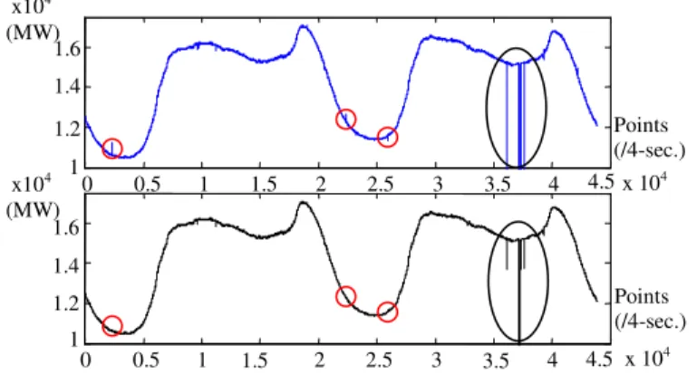
Figure 2-1 depicts the four-second load series before and after the micro spike filter

16

as marked by the three small red circles) are removed by the filter. Spikes with widths

close to or greater than the processing window w1 (macro spikes, as marked by the large

black ellipse) are only attenuated or cannot be handled by the micro spike filter at the

four-second time resolution. However, they may become micro spikes after integration,

and can then be handled by the same method at the five-minute resolution. In this way,

all micro spikes within the processing window are detected and replaced by smoothed

loads, whereas the load data outside the window are not touched.

0 0.5 1 1.5 2 2.5 3 3.5 4 4.5 1 1.2 1.4 1.6 1 1.2 1.4 1.6 x104 (MW) x104 (MW) 0 0.5 1 1.5 2 2.5 3 3.5 4 4.5 x 104 Points (/4-sec.) Points (/4-sec.) x 104

Figure 2-1. Before (top) and after (bottom) micro and macro spike filtering based on two days of continuous ISO-NE load data at the four-second resolution

2.3.2 Macro Spike Filtering

The key idea for filtering out macro spikes is to detect a pair of edges, and fix the

loads between the two edges with linear interpolation values. This method is only applied

to the loads at the five-minute resolution because macro spikes at the four-second

resolution may become micro spikes after integration. To detect edges, the first-order

differencing transformation is applied to the load series at the five-minute resolution.

17

threshold m. A macro spike is then said to be recognized when two sequential edges are

located, and the width of the two edges is less than a threshold w2 and equal to or greater

than the threshold w1. The spike whose width is less than w1 is a micro spike, and should

have been removed in micro spike filtering which is described in Subsection 2.2.1. To

fix a macro spike, the load in-between the two edges is replaced by a value from linear

interpolation. This interpolation method is used because the changes of five-minute loads

over a short time period have similar slopes for most of the times based on observation.

Figure 2-2 depicts the five-minute load series (four-second integrated into five-minute

loads depicted in the second plot of Figure 2-1) before and after the macro filtering is

applied. 0 100 200 300 400 500 600 1 1.2 1.4 1.6 1.8 0 100 200 300 400 500 600 1 1.2 1.4 1.6 1.8 x10 (MW) 4 4 x10 (MW) Points (/5-min.) Points (/5-min.)

Figure 2-2. Before (top) and after (bottom) macro spike filtering at the five-minute resolution

2.4

Wavelet Neural Networks

To perform accurate predictions after pre-filtering, load properties are analyzed in

18

very fast changing component from five to fifteen-minute resolutions, a fast changing

component from fifteen-minute to one-hour resolutions, and a slow changing component

with hourly, weekly, and monthly patterns. The WNN method is developed to capture

the complicated load properties. To accurately capture load features at multiple

frequencies, a wavelet technique is used to decompose the loads into several frequency

components in Subsection 2.4.2. Due to the use of convolution in the wavelet transform,

additional data need to be padded at the end side of the load segment in real-time.

Relationships among the padding parameters are discussed and derived. Different

padding strategies are then tested, and the best one is determined via the test data set. In

Subsection 2.4.3, each load component is properly transformed and then fed with other

time and date indices to a separate neural network. Predictions from individual neural

networks are combined to form the forecasts. Finally, twelve dedicated wavelet neural

networks are used to perform moving forecasts in Subsection 2.4.4.

2.4.1 Load Property Analysis

Very short-term load data have complicated properties. They are illustrated by the

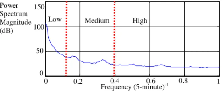
power spectrum density which describes how the power of load data is distributed with

frequency. As shown in Figure 2-3, the main power lies in the low frequency and several

small pedals afterward, and each one has a unique frequency component. Intuitively, this

frequency domain is divided into three frequency components as denoted by low,

medium, and high frequencies. If each one is further magnified by amplitude spectrum

(explained in the next paragraph), it is observed that these components have different

19 Frequency (5-minute)-1 0 0.2 0.8 1 0 50 100 150

Low Medium High

0.4 0.6 Power

Spectrum Magnitude (dB)

Figure 2-3. Power spectrum density for five-minute load data (January 1st, 2007 to June 30th, 2008)

As depicted in Figure 2-4, the amplitude spectrum shows that the low, medium, and

high load frequency components have different features. Spectral lines for the low

frequency component in the eclipse are magnified further. These spectral lines represent

unique load patterns, and the ones located at frequencies corresponding to hourly,

weekly, and monthly information are marked. The amplitude spectrums for the medium

and high load frequencies (reflecting fast changes in load data) have small magnitudes,

and hence are not magnified. Dashed lines are used to separate load components as they

are in the separation in Figure 2-3.

0 0.05 0.1 0.15 0.2 0.25 0.3 0.35 0.4 0.45 0.5 0 0.5 1 1.5 2 2.5 3 3.5 x 104 0 2 4 6 8 x10-3 0 1000 2000 3000 Week 24-hours Season _12-hours Low freq.

Load Amplitude |Y(f)| (MW)

Medium freq. High freq. 1-hour 15-minutes

20

Figure 2-4. Amplitude spectrum for five-minute load data

2.4.2 Filter Bank in Wavelet Transform

The load data have multiple frequency components as depicted in Figure 2-3, and

each may have a unique pattern as depicted in Figure 2-4. An intuitive idea is to

decompose the loads into multiple frequency components and process each

independently. For example, the load data were decomposed into multiple resolution

scales in (Rocha Reis and Alves da Silva, 2005; Benaouda et al., 2006). Fourier

transform is a straightforward technique to represent the signal as a sum of sinusoids

which are only localized in frequency. In contrast to Fourier transform, wavelets are

localized in both time and frequency and often give a better representation using

multi-resolution analysis. A detailed introduction to wavelets can be found in (Mallat, 2009:

Chapter 1). Motivated by the successful one-level wavelet decomposition for short-term

load forecasting in our previous work (Chen et al., 2010), a wavelet technique is chosen

to decompose input loads into multiple frequency components. The input loads are first

decomposed into low (L) and high (H) frequency components at level one. The L

frequency component called "approximation" represents a general trend of the signal,

whereas the H frequency component is viewed as a difference between two successive

approximations (Rocha Reis and Alves da Silva, 2005). Since the load has a large

magnitude and multiple frequency information, the L frequency component is further

decomposed into low-low (LL) and low-high (LH) frequency components. There is no

need to decompose the H component because it has a small magnitude as compared to the

21

LH, and H are very similar to the low, medium, and high frequencies described in

Subsection 2.4.1.

To implement the two-level wavelet transform, a three-channel filter bank is used

as shown in Figure 2-5. The high frequency channel consists of the analysis and

synthesis stages. At the analysis stage, a high pass filter (a wavelet function that plays

the role of the anti-alising) G1 filters out the low frequency component. A

down-sampling step then removes the odd-numbered data points. At the synthesis stage, the

up-sampling step pads zeros to down-sampled data to recover the data length. A high

pass filter H1 then removes the replicas of signal spectrum caused by up-sampling.

Similarly, the low-high frequency channel uses a low pass filter G0 to compute the

general trend, and then holds the even-numbered points. Next, these points are further

decomposed into two parts. The low-high part convolves with G1 and then takes steps

similar to those for the high frequency channel. To recover the initial input length, the

output from H1 has to be up-sampled and convolve with H0. These are the steps to

produce the LH frequency component. The same is true for the low-low frequency

channel. Filters G0, G1, H0, and H1 have to satisfy perfect reconstruction and

orthogonality in (Strang and Nguyen, 1997).

H0 G0 G1 ↑2 H ↑2 H0 LL ↓2 G1 G0 ↓2 ↓2 ↑2 H1 H1 H0 ↑2 ↓2 ↑2 LH Synthesis Stage Analysis Stage Loads

22

The filter bank in the wavelet transform described above adopts a circular

convolution as explained in (Strang and Nguyen, 1997: Chapter 8). Circular convolution

causes boundary distortions which affect neural network predictions. To reduce the

distortion, it is necessary to extend the signal beyond the boundaries. In the high

frequency channel shown in Figure 2-5, the distortion length for a convolution between

the input loads and G1 is (lw-1) based on the convolution theory, where lw is the filter

length. Down-sampling and up-sampling do not produce the distortion. H1 introduces

another distortion with the same length (lw-1). The total distortion length is 2(lw-1). The

low-high frequency channel sequentially convolves the inputs with four filters (G0, G1,

H1, and H0) with a final length of the distortion 4(lw-1), doubling that of the high

frequency channel. The same is true for the low-low frequency channel. The distortion

length is thus roughly doubled for a component which is further decomposed one more

level. A detailed analysis can be found in (Guan and Luh, 2010). To make sure that at

least one value is not affected by distortion, the load inputs to NN need to be padded.

The padding length has to be equal to or greater than the distortion length (wmaxlev

function in MATLAB Wavelet Toolbox):

(

)

lx= −1⋅2 , (3)

where lx is the distortion length which indicates the minimum padding length, and lvl is

the level of the decomposition. Hence, the total length for load inputs to be decomposed

has to be equal to or greater than the sum of the minimum padding length lx and the

length of the load inputs of the last hour (12 points). For VSTLF, the latest historical

data are available and used to pad the last hour’s loads at the front. Additional data are

23

From (3), the relationships among the decomposition level lvl, the filter (G and H) length

lw, and the minimum padding length lx are very close. It can be concluded that fixing lvl

and increasing lw, or vice versa, will increase lx. This indicates that the padding length

will increase, which may not be good because a long padding to load inputs can result in

a poor training and prediction for NN. However, lvl should not be too small because the

features of load components cannot be fully captured. The same is true for lw because a

small lw has a poor ability to represent the load component behaviors. It is clear that

neither lw nor lvl should be too large or small, so that a reasonable lx can be obtained.

Therefore, a balance among lvl, lw, and lx has to be made due to their close relationships

in (3).

To choose a good lvl for decomposition, different values are tested and compared,

while lw and lx remain fixed. Two-level decomposition is found to be the best among

levels from zero to three in Example 2 in Section 2.5. This corresponds to the scheme

presented in Figure 2-5 with three decomposed frequency components H, LH, and LL.

To choose a good filter length lw, a proper wavelet has to be chosen using the previous

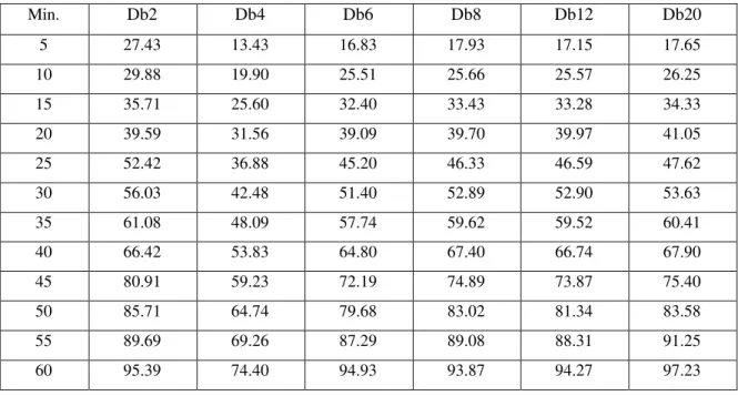
fixed lx and newly determined lvl (=2). Daubechies (Db) wavelets are adopted in our

method because they belong to a family of orthogonal wavelets and are characterized by

frequency responses having maximum flatness (at 0 and π). Db members tested are

Db2-Db20 (even index numbers only). The index number refers to the filter length lw, and

has the ability to represent complicated behaviors of signal components. For example,

Db2 encodes constant components, and Db4 encodes constant and linear ones. However,

the Db number cannot be too large. Otherwise, the minimum padding length will

24

similar slopes for most of the times. Hence, Db4 seems to be a reasonable choice

because it encodes linear signal components, and is demonstrated to be the best among all

the index numbers tested as presented in Section 2.5.

Once lvl (=2) and lw (=4) are fixed in equation (3), lx can be calculated ((lw

-1)·2lvl=12). Since the last hour’s loads (12 points) are used as NN inputs, the total length

for load inputs to be decomposed has to be equal to or greater than the sum of the

minimum padding length and the length of the last hour’s loads (i.e., the total length

≥24). A more precise number can be calculated from the derivation in (Guan and Luh,

2010). To further reduce distortion effects, padding strategies (e.g., zero-padding,

periodic extension, and symmetrization) are tested. According to the test in Example 2 in

Section 2.5, symmetrization, a boundary replication which pads the loads by adding

points symmetric to the original, is demonstrated to be the best strategy. This also

corresponds with the conclusion on page 263 in (Strang and Nguyen, 1997). These

parameters are determined through training, validation, and test processes in a three way

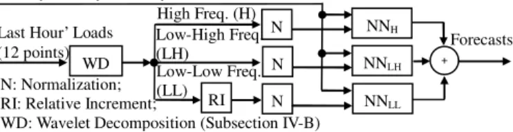
data split. NNH NNLH NNLL + High Freq. (H) Low-High Freq. (LH) Low-Low Freq. (LL) WD Forecasts N RI N N N: Normalization;

RI: Relative Increment;

WD: Wavelet Decomposition (Subsection IV-B) Last Hour’ Loads

(12 points)

Hourly, Weekly, Monthly, and Sunset Time Indices

Figure 2-6. Structure of wavelet neural networks

2.4.3 Neural Networks

To capture decomposed frequencies, our idea is to properly transform individual

25

to separate neural networks. Finally, individual predictions from NNs are added to form

the forecasts as depicted in Figure 2-6.

The load components are treated differently. The LL frequency represents the

majority of load information, including hourly, weekly, and monthly patterns as analyzed

in Subsection 2.4.1. Since the loads from 5 to 60 minute outs are predicted each time, the

loads of the last hour (lag=12) are used as inputs. Loads with other lags are also tested,

but the results are not further improved. To remove a first-order trend and anchor the

predictions by the latest load, the relative increment (RI) in loads in (Charytoniuk and

Chen, 2000), is applied:

( )

(

( )

( )

)

( )

LLRI_{d d d d} , (4)

where LL represents the low-low frequency load component at day index d, and t is the

time index in a five-minute period. RI indicates the relative increment transformation

and is used to stationarize the load component series. This transformation reveals more

of the hidden information in the LL frequency component in Figure 2-7.b than the one

without applying RI in Figure 2-7.a. But the other observation shows that RI reveals less

of hidden information in the LH and H components than the one without applying RI.

Hence, RI transformation is only applied to the LL load component. All the components

then have to be normalized and fed to individual NNs.

0 0.1 0.2 0.3 0.4 0.5 0 0.005 0.01 0 0.1 0.4 0.5 0 0.005 0.01 7.a 7.b Normalized Low-Low Frequency Load Amplitude |Y(f)| (MW) Frequency (5-minute)-1

26

Figure 2-7.a. Amplitude spectrum for normalized low-low frequency before applying RI; Figure 2-7.b. Amplitude spectrum for normalized low-low

frequency after applying RI

In addition to load inputs (5 to 60 minutes), time and date indices are parts of the

neural network inputs, including hourly, weekly, and monthly indices. Furthermore,

sunset time is included to capture the load feature related to the street lighting. These

indices are used to help NNs indentify the periodical patterns of load data. Similarly,

low-high and high frequency NNs adopt the same time and date indices but use the load

components without RI transformation. Finally, results from three NNs are summed up

to form final forecasts. Other additional inputs were tested but not considered because

the results were not significantly improved. These inputs include: area control errors,

frequencies, and some selected loads from history (e.g., loads of the last several hours,

loads of selected hours from yesterday, similar day’s loads, and so on). Based on the

literature review, actual weather data and weather forecasts from related methods, e.g.,

the climatology method (weather world 2010 project), are seldom used for VSTLF inputs

because of the large time constant of the load and weather relationship. Also, real-time

weather data are not available from ISO New England.

To narrow the numerous choices of input candidates down, different combinations of

data inputs are screened based on small data sets. For example, load data from

November 2007 to December 2007 are used for training, and loads for January 2008 are

then predicted. The resulting candidate inputs are then examined through training,

27

2.4.4 Moving Forecasts

When performing moving forecasts every five minutes, the intuitive approach

would be to train a single WNN offline with historical data as presented in (Haykin,

2009: Chapter 4) and train the WNN online whenever a new data point is available. This

is the same as the self-adaptive training process of (Herrera et al., 2010). However, test

results using this approach are not satisfactory. Based on further testing, our final

configuration consists of twelve dedicated WNNs, one for each five-minute period in the

hour. In this way, individual WNNs can be properly trained. For example, at 2:55 am,

WNN1 predicts the loads from 3:00 am to 3:55 am in five-minute periods; WNN2 at time

3:00 am predicts the loads from 3:05 am to 4:00 am in five-minute periods, etc. Then at

3:55 am, when the measured values are known for the past 12 time steps, WNN1 is

trained online (updated) with the data from 3:00 am to 3:55 am and then predicts the

loads from 4:00 am to 4:55 am, and the process repeats.

2.5

Numerical Test Results

The method was developed in MATLAB for prototype implementation and then

converted to JAVA using Eclipse. The open source can be downloaded at

http://github.com/ldmbouge/vstlf. In this section, the software was run on a server with

dual Xeon quad core Intel E5620 2.4GHz processors and 36 GB memory. The

performance measures include mean absolute error (MAE), mean absolute scaled error

(MASE) as presented in (Hyndman and Koehler, 2006; Hyndman, 2006), mean average

percentage error (MAPE), and standard deviation of sample errors (SD):

( )

( )

( )

28

( )

MASE = ( ) _{− − −} , (6)

( )

(

( )

( )

( )

)

( )

[

(

( )

(

( )

( )

)

)

]

In the above equations, index k represents 5 to 60 minutes in five-minute steps, n

indicates the number of hours in the forecasting horizon, and LA(t) and LP(t) denote actual

and predicted loads at sample time t, respectively. The general performance measures

include MAE, MAPE, and SD. MASE provides a scale-free error metric for comparing

forecasting methods on a single series (Hyndman and Koehler, 2006). In (6), the

numerator MAE(k)out-of-sample for k-step out (k = 1, …, 12) is calculated for the multistep

WNN forecasts computed out-of-sample (in the testing data set). The denominator

MAEin-sampleis calculated for the one-step "naïve forecast" computed in-sample (in the

training and validation data sets). The naïve forecast for each future period is the actual

value for the previous period (Hyndman, 2006). This denominator MAEin-sampleis used to

scale the numerator MAE(k)out-of-sample to generate a scale-free error metric that is stable,

easy to compute, and in the correct unit. If the MASE value is less than one, this

indicates that the forecast of the presented method is better than the one-step naive

forecast. However, if the MASE value is greater than one, this indicates the opposite.

Multistep MASE values are often larger than one as the forecasting horizon increases

because one step naive forecast is used for scaling (Hyndman and Koehler, 2006;

Hyndman, 2006). Equations (5) to (8) can also be applied to moving forecasts with

multiple WNNs.

Two examples are presented to demonstrate our method. Example 1 uses a

29

so that our method can be duplicated and verified in a simple way. Example 2

demonstrates the values of spike filtering methods, two-level decomposition, Db4

wavelet, Symmetrization padding, selected time and date indices (hourly, weekly,

monthly, and sunset time), and relative increment transformation to the LL frequency

component.

In both examples, standard neural networks based on the back-propagation learning

algorithm in (Haykin, 2009: Chapter 4) are used. The training, validation, and test

processes in a three way data split are used to determine and demonstrate the parameters

in the model. All NNs are trained offline by using historical data with weights randomly

initialized, and the training terminates when the stopping criteria is reached to be

described in Examples 1 and 2. These NNs are then trained online with the latest twelve

loads as explained in Subsection 2.4.3

Example 1.Consider the signal:

( )

(

)

(

)

(

)

y π π π , (9)

where the signal y(t) is composed of a low frequency component 100sin(2π10t), a

medium component 20sin(2π150t), and a high component sin(2π200t). The signal is

similar to the actual load in terms of relative amplitude and frequency. A total of 3600

data points (t, ỹ(t)) were randomly generated:

( ) ( ) ( )

~ _{, (10)}

where t ∈ [1, …, 3600] and {ε(t)} were independent and identically distributed normal noises with zero mean and unit variance N(0, 1). The first one-third of data points were

30

used for training, the second one-third of data for validation, and the last one-third of data

for testing.

A single NN without wavelet decomposition is compared to neural networks with

two-level wavelet decomposition. The relative increment transformation is not used for

this example because y(t) consists of three sine functions which are periodical, and there

is no need to use this transformation to make {y(t)} stationary. Based on the training,

validation, and test processes in a three way data split, the number of hidden neurons for

the standard NN method is set to be 11, and the numbers of hidden neurons for our

method are set to be 8, 7, and 13 for H, LH, and LL NNs, respectively. For both

methods, NN training processes stop when MAE thresholds (stopping criteria) are

reached. From the test data set, the overall MAE and SD are respectively 1.73 and 2.33

for standard NN method, whereas the overall MAE and SD are respectively 0.85 and 1.06

for our method. MAPE is not adopted since {y(t)} may have zero values. MAEs and

SDs indicate that the predictions obtained from using two-level wavelet NNs are both

closer to the true values in data series {y(t)} and have smaller standard deviations than

the ones obtained using a single NN.

Example 2. Wavelet neural networks with spike filtering are tested with system load

data provided by ISO New England. The training period is from January 1st, 2007 to

December 31th, 2007, the validation period is from January 1st, 2008 to June 30th, 2008,

and the test period is from July 1st, 2008 to December 31th, 2009. Ten cases are tested.

Since there are many factors in setting the forecasting model, and each factor has

31

practical way to demonstrate the appropriateness of options selected for individual

factors, the configuration determined through training, validation, and test processes is

treated as the nominal configuration. Based on it, each factor is then examined in

individual cases below. Cases 1 -7 are for training and validation: Case 1 for micro and

macro spike filtering, Case 2 for spike filtering thresholds, Case 3 for decomposition

levels, Case 4 for selecting Daubechies wavelets, Case 5 for padding strategies, Case 6

for date and time indices, and Case 7 for relative increment transformation. Cases 8-10

are for testing: Case 8 for test results and prediction interval construction, Case 9 for

comparing with ISO-NE’s method, and Case 10 for Monte Carlo simulations.

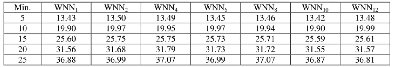
To reduce computation time, Cases 3-7 are based on WNN1 because its results are

very similar to the individual results from other WNNs as reported in Table 2-1, while the

other cases are based on the twelve dedicated WNNs. For all the cases, there are three

layers in all the neural networks: one input layer, one hidden layer, and one output layer.

Through training, validation, and test processes in a three way data split, the numbers of

hidden neurons are 6, 13, and 18 for H, LH, and LL NNs, respectively. They are not

identical because the decomposed load components have different features. Based on

testing, a single WNN is trained offline for three hours (stopping criterion), and twelve

WNNs require a total of thirty six hours for training offline.

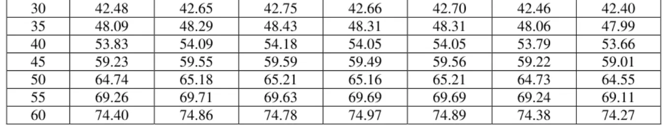
Table 2-1. MAES (MW) FOR MULTIPLE WNNS

Min. WNN1 WNN2 WNN4 WNN6 WNN8 WNN10 WN