Individual Risk Attitudes: New Evidence from a Large,
Representative, Experimentally-Validated Survey
Thomas Dohmen1, Armin Falk2, David Huffman1, Uwe Sunde2
J¨urgen Schupp3, Gert G. Wagner4 November 11, 2005
Abstract
This paper presents new evidence on the distribution of risk attitudes in the pop-ulation, using a novel set of survey questions and a representative sample of roughly 22,000 individuals living in Germany. Using a question that asks about willingness to take risks in general, on an 11-point scale, we find evidence of heterogeneity across individuals, and show that willingness to take risks is negatively related to age and being female, and positively related to height and parental education. We test the behavioral relevance of this survey measure by conducting a complementary field ex-periment, based on a representative sample of 450 subjects, and find that the general risk question is a good predictor of actual risk-taking behavior. We then use a more standard lottery question to measure risk preferences in our sample of 22,000, and find similar results regarding heterogeneity and determinants of risk preferences, compared to the general risk question. The lottery question also makes it possible to estimate the coefficient of relative risk aversion for each individual in the sample. Using five questions about willingness to take risks in specific domains — car driving, financial matters, sports and leisure, career, and health — the paper also studies the impact of context on risk attitudes, finding a strong but imperfect correlation across con-texts. Using data on a collection of risky behaviors from different contexts, including traffic offenses, portfolio choice, smoking, occupational choice, participation in sports, and migration, the paper compares the predictive power of all of the risk measures. Strikingly, the general risk question predicts all behaviors whereas the standard lot-tery measure does not. The best predictor for any specific behavior is typically the corresponding context-specific measure.
Keywords: Risk Preferences, Experimental Validation,
Field Experiment, SOEP, Gender Differences, Context, Age, Height, Subjective Well-Being, Migration,
Occupational Choice, Health
JEL codes: D0, D1 D80, D81, C91, C93, J16, J24, J61, I1
1
Institute for the Study of Labor (IZA); e-mail: dohmen@iza.org; huffman@iza.org;
2 IZA and University of Bonn; e-mail: falk@iza.org; sunde@iza.org
3
German Institute for Economic Research (DIW); e-mail: jschupp@diw.de
4 DIW, Berlin University of Technology, and Cornell University; e-mail: gwagner@diw.de
Corresponding Author: Armin Falk, IZA, P.O. Box 7240, D-53072 Bonn, Germany. e-mail: falk@iza.org
1
Introduction
Risk and uncertainty are pervasive in economic life, playing a role in almost every impor-tant economic decision. As a result, understanding individual attitudes towards risk is intimately linked to the goal of predicting economic behavior. This paper uses a powerful combination of data – a large, representative survey and a representative field experiment designed to validate the survey measures – in order to provide more definitive answers to some of the challenging questions surrounding this concept in the literature. In particular, do risk attitudes vary across individuals? If so, what are the determinants of individ-ual differences? Are hypothetical measures of risk attitudes reliable predictors of actindivid-ual risky behavior? What is the impact of context on willingness to take risks? Is there a single underlying preference that determines risk-taking in all contexts? How does the impact of personal characteristics vary with context? Can survey questions incorporating situation-appropriate context outperform standard lottery measures of risk preference?
Our evidence is based on a sample of roughly 22,000 individuals. The data are from the 2004 wave of the Socioeconomic Panel (SOEP), which is carefully constructed to be representative of the German population. For each individual, the data provide a battery of new survey measures. The first measure asks about “willingness to take risks, in general” on an 11-point scale. The second is a more standard lottery measure of risk preference, in which respondents indicate willingness to invest in a hypothetical asset with explicit stakes and probabilities. Assuming the existence of a canonical utility function, it is possible to use responses to this question to calculate a parameter describing the curvature of utility for each individual. There are also five additional questions, which use the same scale as the general risk question, but ask about willingness to take risks in specific contexts: car driving, financial matters, sports and leisure, career, and health. In a complementary field experiment, based on a representative sample of 450 individuals, we test the behavioral relevance of the general risk question, and find that it is a good predictor of risky choices with real money at stake. As a result of the experimental exercise, we can be confident about the behavioral validity of this measure and other similar measures in the SOEP.
The paper begins by presenting new evidence on the distribution of risk attitudes in the population, and the determinants of individual differences. Initially, we focus on our most general measure, the general risk question, and construct a population-wide
distribution of willingness to take risks. This distribution reveals substantial individual heterogeneity. Turning to possible determinants of these differences, we investigate the relationship between willingness to take risks and selected personal characteristics: gender, age, height, and parental background. We focus on these characteristics because they are plausibly exogenous and therefore allow causal interpretation. The analysis reveals several facts: (1) women are less willing to take risks than men, at all ages; (2) increasing age is associated with decreasing willingness to take risks; (3) taller individuals are more willing to take risks; (4) individuals with highly-educated parents are more willing to take risks. These effects are large, robust, and have important implications. For example, differences in risk preferences could be one factor contributing to the well-known gender wage gap, and could help explain gender-specific behavior in competitive environments (Gneezy et al., 2003; Gneezy and Rustichini, 2004), and gender differences in career choice (Dohmen and Falk, 2005). The impact of age implies increased financial conservatism in ageing societies, and the height result points to a possible mechanism behind the higher earnings potential of taller individuals (Persicoet al., 2004). These findings also suggest characteristics that can be used to partially control for risk attitudes in the absence of direct survey measures. A chief advantage of survey questions is that they offer a direct measure of individual attitudes, avoiding the need to use behavioral proxies or recover behavioral parameters by making restrictive identifying assumptions. Another advantage is the possibility of measuring attitudes for a very large sample, at relatively low cost in terms of money and time: survey questions are hypothetical and thus do not involve real money, and are relatively easy to explain and administer. A potentially serious disadvantage of using hypothetical survey questions, however, is that they might not predict actual behavior. In this paper we offer a solution to this dilemma. The primary methodological point of the paper is that field experiments with a representative subject pool can be used to validate the survey measures in much larger, representative samples, in order to end up with both statistical power and confidence in the reliability of the measures. To test the validity of our survey measures, we conducted a field experiment in which participants had the opportunity to make risky choices with real money at stake, and also answered the general risk question from the SOEP. We used a representative sample of 450 adults living in Germany as subjects, in order to match the sampling design of the survey. We find that answers to the general risk question are good predictors of actual risk-taking
behavior in the experiment. We can therefore be confident in the behavioral relevance of the measure.
It is important to compare results based on the general risk question to results using a more standard lottery measure. The SOEP poses respondents with such a lottery, in the form of a hypothetical investment opportunity: respondents are asked how much of a windfall gain of 100,000 Euros they would invest in an asset that returns double, or half, of their investment, with equal probability. In comparison to the general risk measure, this question incorporates the relatively concrete context of a real-world financial decision. It also gives explicit stakes and probabilities, holding perceptions of the riskiness of the decision constant across individuals. The amount invested in the hypothetical asset turns out to be strongly correlated with responses to the general risk question. The distribution of investment choices reveals heterogeneity across individuals, and gender, age, height and parental education all play a role in explaining differences in risk preferences. The effects of all of these exogenous factors are very robust and qualitatively similar to those observed using the general risk question.
Assuming the existence of a CRRA utility function, and combining responses to the lottery question with information on individual wealth, it is also possible to calculate, for each individual, a parameter that describes the curvature of utility. This parameter cor-responds to the notion of risk preference in expected utility theory, where the willingness to take a given gamble is derived from the curvature of utility in lifetime wealth. We construct a distribution of interval midpoints in the population, and find that it is roughly consistent with the range of parameter values typically assumed in economic models. We also illustrate the first step needed to interpret responses to the general risk question in terms of ranges for parameter values: a mapping from responses on the general risk ques-tion to average amounts invested in the hypothetical asset, which then imply parameter ranges.
A fundamental question surrounding the notion of risk attitudes is the relevance of context. In economics it is standard to assume that a single, underlying trait governs risk taking in all domains of life. In line with this assumption, economists typically use a lottery measure of risk preference, framed as a financial decision, as an indicator of risk attitudes in all other contexts, e.g., health or career. There is mixed evidence from laboratory experiments, however, on whether a stable risk trait exists at all: in some studies risk
attitudes appear to be highly malleable with respect to context (for a discussion see, e.g., Slovic, 1964, 1972a and 1972b).
The five context-specific questions in the SOEP make it possible to study the impact of context, but for a much larger and more representative group of individuals than the typical laboratory experiment. Average willingness to take risks turns out to differ across contexts. However, the correlation across contexts is quite strong. Principal components analysis tells a similar story: one principal component explains the bulk of the variation, suggesting the presence of a single underlying trait, but each of the other components still explains a non-trivial amount of the variation. Overall, these findings support a middle position between the two extreme views. There is evidence for a single trait operating in all contexts, suggesting that the standard assumption is a reasonable approximation. On the other hand, something is varying across contexts. This could reflect some malleability in risk preferences, but we argue that it is more likely to reflect differences in risk perception. Like the general risk question, the context-specific measures are able to capture differences in risk perception, e.g., beliefs regarding the relative danger of driving versus playing sports. In fact, risk perceptions are known to vary across individuals based on evidence from psychology.1 The implication is that the standard approach – using lottery questions to predict behavior in all contexts – may be reasonable to the extent that it captures a stable risk trait, but also neglects some potentially important variation in context-specific willingness to take risks.
The final portion of the analysis compares the predictive power of all of the alter-native risk measures, within and across different life contexts. We identify a collection of behavioral outcomes that spans the five contexts identified in the SOEP — portfolio choice, participation in sports, occupational choice, smoking, migration, subjective well-being, and traffic violations — and then compare how well different risk measures do at predicting these behaviors. The first finding is that any single measure is a significant predictor of several of the behaviors, providing further validation of their behavioral rel-evance. This validity across contexts also supports the standard assumption of a stable,
1 For example, a number of studies have asked directly about risk perceptions and have documented a
tendency for women to perceive dangerous events, such as nuclear war, industrial hazards, environmental degradation, and health problems due to alcohol abuse, as more likely to occur, in conditions where objective probabilities are difficult to determine (Silverman and Kumka, 1987; Stallen and Thomas,
1988; Flynnet al., 1994; Spigneret al., 1993). For laboratory evidence on differences in risk perception,
underlying risk preference. Importantly, however, the only measure to predict all of the behaviors is the general risk question. In this sense the general risk question is the best all-around measure. By contrast, although the hypothetical lottery does successfully predict some behaviors, it does not predict smoking, migration, or self-employment and predicts public sector employment with the “wrong” sign. It is also striking that the best predictor of behavior in a given domain is typically the question incorporating context specific to that domain. For example, willingness to take risks in health matters is a better predictor of smoking than the hypothetical investment question, or the general risk question, or any other domain-specific question. A likely explanation for the better performance of the alternative measures is that they capture additional information about the individual, in terms of context-specific risk perceptions, e.g., the individual’s beliefs regarding the dangers of smoking. Overall, the evidence calls into question the practice of exclusively using lottery questions to predict risky behavior, across all contexts. This approach is only optimal if risk preferences, and risk perceptions, remain constant across contexts, which seems inconsistent with our findings.
In summary, the paper contributes new evidence on the determinants and measure-ment of individual risk attitudes. These conclusions are based on a substantially larger sample than in previous studies, and on survey measures that are shown to be behav-iorally relevant in an accompanying field experiment. As such, the conclusions have a broader scope than in previous studies and can be interpreted in terms of behavior with more confidence. Previous studies using relatively large, representative samples include Guiso et al.(2002), Guiso and Paiella (2001), and Guiso and Paiella (2005), all of whom use a sample of 8,135 heads of households in the Italian Survey of Household Income and Wealth (SHIW) and measure risk preferences with an abstractly-framed, hypotheti-cal lottery. Diaz-Serrano and O’Neill (2004) use the same sample but also add the next wave from the survey, which includes roughly 3,000 additional individuals. Donkerset al.
(2001) use a sample of 4,000 individuals living in the Netherlands, one half of which is representative and the other half of which is drawn from the top 10 percent of the income distribution, and measure risk preferences with a series of abstract lotteries. Barskyet al.
(1997) use an especially large sample, 14,000 individuals living in the US, but this comes from the Health and Retirement Survey which is focused on individuals between 51 and 61 years of age. They measure risk preference using a hypothetical lottery involving different
future income streams. Where it is relevant in the paper, we discuss the methodologies of these complementary studies in more detail.
There are a number of cases in which the evidence in this paper provides a powerful confirmation of previous findings, but others in which the findings contrast strongly with previous results. In particular, many previous studies have found a similar impact of gender on willingness to take risks (for a meta-analysis, see Byrnes et al., 1999; for a review of experimental evidence on gender effects, see Eckel and Grossman, 2003 and Eckel and Grossman, forthcoming). This paper documents the same gender difference on a larger scale, but in contrast to experimental evidence in Schubert et al. (1999), the effect is robust to the inclusion of concrete context in the question frame, e.g., as in the hypothetical investment scenario. In fact, the gender effect is present in all contexts, and at all ages, and is robust to controlling for wealth and other personal characteristics. In terms of the age effect, this paper is one of the few to study the full range of ages over adulthood, (exceptions include studies using the SHIW, Donkerset al., 2001, and Harrison
et al., 2005), and the first to investigate the impact of age in a variety of contexts. Few previous papers have investigated the impact of parental background on risk attitudes, with the exception of Guiso and Paiella (2001), and Guiso and Paiella (2005), who look at father’s occupation (Hartog et al., 2002, finds a similar impact of mother’s education in a sample composed of accountants). To our knowledge, no previous paper has studied the relationship between height and risk attitudes.
The estimates of CRRA coefficients in this paper differ from previous studies in that they incorporate detailed information on individual wealth, and are based on a lottery with stakes that are large enough to be meaningful in terms of lifetime income (for other ap-proaches see Barsky et al., 1997; Donkerset al., 2001; Guiso and Paiella, 2005; Harrison
et al., 2004; Holt and Laury, 2002). The analysis of risk attitudes across contexts has mainly been studied in psychology experiments with much smaller sample sizes. Previous studies have found that standard measures of risk preference predict behaviors such as portfolio choice, smoking, and occupational choice. Our measures have similar predictive power, but our findings also point to the importance of risk perceptions in determining risky behavior. In particular, more comprehensive measures incorporating both risk pref-erence and context-specific risk perceptions outperform a standard lottery measure of risk preference.
The organization of the paper is as follows. Section 2 describes the SOEP and the risk measures. Section 3 investigates individual heterogeneity and exogenous determinants of risk attitudes using the general risk question. Section 4 presents results on the behav-ioral relevance of the general risk question, based on the complementary field experiment. Section 5 compares the distribution and determinants of investment choices in the hypo-thetical lottery to results based on the general risk measure, and calculates individual risk coefficients. Section 6 assesses the stability of risk attitudes across different domains of life. Section 7 compares the predictive power of the different risk measures for a collection of behavioral outcomes. Section 8 concludes.
2
Data Description
The SOEP is a representative panel survey of the resident population of Germany (for a detailed description, see Wagner et al., 1993, and Schupp and Wagner, 2002). The initial wave of the survey was conducted in 1984.2 The SOEP surveys the head of each household in the sample, but also gives the full survey to all other household members over the age of 17. Respondents are asked for a wide range of personal and household information, and for their attitudes on assorted topics, including political and social issues. The survey also includes various subjective measures (e.g., life satisfaction) which are widely used and recognized for their quality (see, e.g., Ferrer-i-Carbonell and Frijters, 2004; Frijterset al., 2004a and 2004b; van Praag and Ferrer-i-Carbonell, 2004). This paper is the first to use the new measures of risk attitudes added to the survey in the 2004 wave. The 2004 wave, which includes 22,019 individuals in 11,803 different households, is the focus of our analysis.
We analyze seven different questions from the SOEP which ask, in different ways, about an individual’s risk attitudes. The first question asks for attitude towards risk in general, allowing respondents to indicate their willingness to take risks on an eleven-point scale, with zero indicating complete unwillingness to take risks, and ten indicating complete willingness to take risks.3 The next five questions all use the same scale, and
2
The panel was extended to include East Germany in 1990, after reunification. For more details on the SOEP, see www.diw.de/gsoep/.
3 The exact wording of the question (translated from German) is as follows: How do you see yourself:
“Are you generally a person who is fully prepared to take risks or do you try to avoid taking risks? Please tick a box on the scale, where the value 0 means: ‘unwilling to take risks’ and the value 10
similar wording, but refer to risk attitudes in specific contexts: car driving, financial matters, leisure and sports, career, and health. All of these measures are characterized by ambiguity, in the sense that they leave it up to the respondent to imagine the typical probabilities, and stakes, involved in taking risks in a given domain.
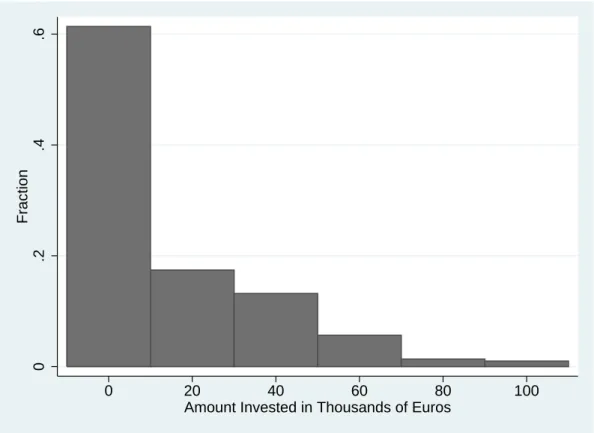
The last risk question is different, in that it corresponds more closely to the lottery measures used in previous studies. The question presents respondents with a hypothetical situation, in which they have just won 100 thousand Euros in the lottery. Immediately after collecting the winnings, a reputable bank contacts them and offers them the opportunity to invest some or all of the money in a risky asset, which doubles the amount invested, or returns only half, with equal probability in two years. Respondents are then asked what fraction of the 100,000 Euros they would choose to invest, and are allowed six possible responses: 0, 20,000, 40,000, 60,000 80,000, or 100,000 Euros.4 This measure is similar to other lottery measures typically used in the literature, in that it presents respondents with a gamble involving explicit stakes and probabilities, and thus holds risk perceptions constant across individuals. Because beliefs are held constant, differences in responses are attributable to risk preference alone, as compared to the six measures above, which potentially incorporate both risk preference and risk perceptions. One feature of the lottery question that deserves additional comment is the two-year lag between the time of investment and the hypothetical payoff. On the one hand this feature is necessary to create the context of a realistic investment. On the other hand there is a potential confound, if time preferences play a role in people’s answers to the investment question, and time preference is systematically related to risk preferences for an individual. In Dohmen
et al. (2005), however, we analyze data from a field experiment, in which we elicit time preferences as well as questionnaire answers to the general risk question discussed above. It turns out that the correlation between elicited time preferences and stated risk preferences is not significantly different from zero, ameliorating this concern. Assuming the existence means: ‘fully prepared to take risk’.” German versions of all risk questions are available online, at www.diw.de/deutsch/sop/service/fragen/personen/2004.pdf.
4
The exact wording (translated from German) is as follows: “Please consider what you would do in the following situation: Imagine that you had won 100,000 Euros in a lottery. Almost immediately after you collect the winnings, a reputable bank offers you the following investment opportunity, the conditions of which are as follows: You can invest money. There is the chance to double the invested money within two years. However, it is equally possible that you could lose half of the amount invested. You have the opportunity to invest the full amount, part of the amount or reject the offer. What share of your lottery winnings would you be prepared to invest in this financially risky, yet potentially lucrative investment?”
of a canonical utility function, it is also possible to use responses to the hypothetical lottery to infer a parameter describing the curvature of the individual’s utility function, corresponding to the theoretical notion of risk preference in expected utility theory.
3
Willingness to Take Risks in General
This section presents the distribution of willingness to take risks in the population, as measured by the general risk question, and then turns to the investigation of possible determinants of individual differences in risk attitudes.
3.1 Risk attitudes in a representative sample
Figure 1 describes the distribution of general risk attitudes in our sample. Each bar in the histogram indicates the fraction of individuals choosing a given number on the eleven point risk scale. The modal response is 5, but a substantial fraction of individuals answers in the range between 2 and 8. There is also a notable mass, roughly 7 percent of all individuals, who choose the extreme of 0, indicating a complete unwillingness to take risks. Only a very small fraction chooses the other extreme of 10.
3.2 Exogenous Factors: Gender, Age, Height and Parental Education
Given that risk attitudes are heterogeneous, it is important to understand the determinants of these individual differences. We investigate the impact of four personal characteristics on risk attitudes: gender, age, height, and parental background. We focus on these char-acteristics because they are plausibly exogenous to individual risk attitudes and behavior and thus allow us to give a causal interpretation to correlations and regression results.5
The lower panel of Figure 1 shows the difference between the fraction of women and the fraction of men choosing each value on the general risk scale. Clearly, women are more likely to choose low values on the scale and men are more likely to choose high values. The figure thus gives an initial indication that women are less willing to take risks than men.
5 Note, however, the caveat that age could potentially be endogenous, for example if people who are less
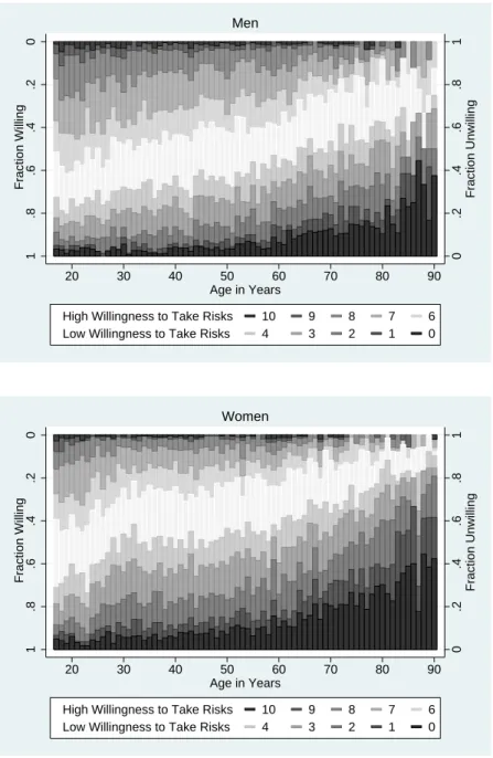
Figure 2 displays the relationship between age and risk attitudes, with separate panels for men and women. The shaded bands indicate the proportion of individuals at each age who choose a given value on the 11-point risk scale. Starting at the bottom, the darkest shade shows the proportion choosing 0, indicating a complete unwillingness to take risks. Progressively lighter shades correspond to choices 1 to 4, and the white band corresponds to 5. Above the white band, progressively darker shades indicate choices 6 to 10.
Clearly, the proportion of individuals who are relatively unwilling to take risks, i.e., choose low values on the scale, increases strongly with age. For men, age appears to cause a steady increase in the likelihood that an individual is unwilling to take risks. For women, there is some indication that unwillingness to take risks increases more rapidly from the late teens to age thirty, and then remains flat, until it begins to increase again from the mid-fifties onwards. It is important to note that this relationship could reflect a direct effect of age on risk preferences, but could also be driven by cohort effects, i.e., society-wide changes in risk preferences over time, perhaps due to major historical events. The difference in age patterns for men and women makes it less credible that the change in risk attitudes is attributable to cohort effects, because major historical events are likely to affect both men and women at the same time, but it is difficult to definitively disentangle the two explanations with the data available.
Comparing the panels for men and women, it appears that women are less willing to take risks than men at all ages, although the gap narrows somewhat among the elderly. Another noteworthy feature of Figure 2 is that the differently shaded bands track each other quite closely over the entire age range. This suggests that aggregating the risk measure from eleven categories to a smaller number of categories is likely to preserve most of the information in the risk measure. This observation will lead us to adopt a simple, binary classification of risk attitudes in parts of the analysis later on.
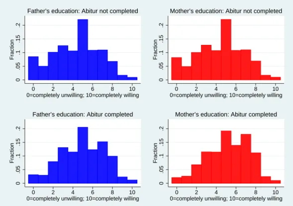
Figure 3 presents histograms of responses to the general risk question by parental education. Other aspects of family background could be relevant for risk attitudes, e.g., parental income, but only parental education is available in the data.6 As a proxy for highly-educated parents, we use information on whether or not a parent passed theAbitur, an exam that comes at the end of university-track high school in Germany and is a
site for attending university.7 The histograms in Figure 3 give some indication that family background does play a role in determining risk attitudes. The mass in the histograms for individuals with highly-educated parents, shown in the bottom panel, appears shifted to the right compared to histograms for individuals without highly-educated parents, shown in the upper panel, indicating a positive correlation between parental education and will-ingness to take risks.
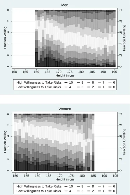
Figure 4 presents histograms of responses to the general risk question by self-reported height, again with separate panels for men and women. The figure shows that taller individuals are more willing to take risks. This relationship is unconditional, and thus could reflect correlation with other factors, in particular parental education. For example, highly-educated parents might have higher income, provide better nutrition, and thus have taller children.8 On the other hand, the result could reflect a direct effect of height on willingness to take risks, perhaps through a channel discussed recently in Persico et al.
(2004). They find that individuals who are tall in their teenage years earn higher wages later in life, even if they are the same height in adulthood. They hypothesize that this difference is due to the impact of height in adolescence on confidence and self-esteem. Our findings suggest one channel through which the greater confidence arising from height translates into positive economic outcomes: increased willingness to take risks.
3.3 The Joint Role of Exogenous Determinants
To determine whether these unconditional results are robust once we control for all four exogenous characteristics simultaneously, we turn to regression analysis. We estimate bi-nary Probit models, where the dependent variable is equal to 1 if individuals are relatively willing to take risks, i.e., choose a value greater than 5 on the risk scale. Likewise, a person is classified as relatively unwilling to take risks if he or she chooses a value of 5 or lower on the risk scale. We prefer using this binary measure, despite the fact that it neglects some information contained in the ordinal structure, because it generates results that are intuitive and simple to interpret, and minimizes problems arising from individual-specific
7
There are two types of high school in Germany, vocational and college-track. Only about 30 percent
of students attend college-track high schools, and pass their Abitur, allowing them to attend college.
Thus, completion of anAbitur exam is an indicator of relatively high academic achievement.
8
Height is frequently used as an instrument for child nutrition and health in the development literature see, e.g., Schultz (2002).
differences in the use of response scales.9 All estimation results report robust standard errors, corrected for possible correlation of the error term across individuals from the same household. The only sample restriction in the analysis is the omission of individuals who have missing values for any of the variables in the regression.
Table 1 summarizes our initial regressions. The baseline specification, presented in Column (1), uses the four exogenous characteristics discussed above as explanatory variables. The resulting coefficient estimates show that the unconditional results remain robust. Women are significantly less willing to take risks in general. The probability that someone is willing to take risks also decreases significantly with age. Unreported regressions that include age in splines with knots at 30 and 60 years reveal that the age effect is particularly strong for young and old ages, reflecting the patterns displayed in Figure 2.10 The inclusion of splines leaves the estimates of the other coefficients virtually unchanged. Taller people are more likely to report that they are willing to take risks. Finally, having a mother or father who is highly educated, in the sense of having completed theAbitur, significantly increases the probability that the individual is willing to take risks. All of these effects are individually and jointly significant at the 1-percent level.11
Columns (2) to (9) check the robustness of our findings by including other control variables. The most important economic variables that need to be controlled for are mea-sures for income and wealth. High income or wealth levels may increase the willingness to take risks because they cushion the impact of bad outcomes. Individual wealth infor-mation is taken from the 2002 wave of the SOEP, which contains detailed inforinfor-mation on different assets and property values.12 Household wealth is constructed by summing the
9
We find similar results if we estimate Ordered Probit, or interval regression models, using a dependent variable that reflects the full range of answers from 0 to 10. For example, if we use an Ordered Probit, the z-values for the exogenous factors in Column (1) of Table (1) are as follows: -13.74 for gender, -29.01 for age, 10.18 for height, 3.34 for mother’s education, and 5.05 for father’s education. Because the results in this and other columns are robust to this alternative estimation method, we feel confident reporting the simpler, more intuitive Probit results.
10
Results for spline regressions are available upon request.
11A likelihood-ratio test reveals that adding interaction terms between all independent variables improves
the fit. The coefficients of interest in the unrestricted specification, however, are very similar to those from the restricted model, both qualitatively and quantitatively. We prefer the model reported in Column 1 of Table 1 for ease of presentation and interpretation, because, e.g., the coefficient on the in-teraction term between age and parental education might be driven by trends in educational achievement over time.
12
The regression includes log individual wealth if wealth is positive (non-zero) and the absolute value of individual wealth logged if wealth is negative (non-zero).
wealth information of all individuals in the household.13 The yearly or monthly income measures ask about income from a variety of sources, including retirement pensions, social assistance, capital and labor income. We use income information from the 2003 as well as from the 2004 wave. The former provides data on annual net income, while the latter has data on current monthly gross income at the stage of the interview. A potential problem with adding these variables to the regression is that they may be endogenous, e.g., a high wealth level could lead to greater willingness to take risks, because it cushions the impact of bad outcomes, but a greater willingness to take risks could also lead to high wealth lev-els. Wealth and income are sufficiently important economic variables, however, that it is arguably important to know what happens to the baseline results when they are included in the regression.
A comparison of the results in Columns (2) to (7) to results in Column (1) shows that the coefficient estimates are very robust to including the additional income and wealth controls. The point estimates for gender, age, height and parental education are virtu-ally unchanged, and remain equvirtu-ally statisticvirtu-ally significant, regardless of which wealth or income measure is included in the regression. Although causal interpretations are inad-visable, it is noteworthy that the correlation between wealth or income and risk attitudes goes in the predicted direction, i.e., these coefficients are invariably positive and significant, indicating that wealthier individuals are more willing to take risks.
As an additional robustness check, Columns (8) and (9) control for wealth and income simultaneously, at the individual or household level, and also add a variety of other personal and household characteristics. These characteristics, which are all potentially endogenous, include among others: marital status, socialization in East or West Germany, nationality, employment status (white collar, blue collar, private or public sector, self-employed, non-participating), education, subjective health status, and religion. For the sake of brevity, the table does not report coefficient estimates for all of the additional controls. The precise specification and all coefficients are shown in Table A.1 in the Appendix. Once again, the point estimates and significance levels for gender, age, and height are virtually unchanged. The coefficients for parental education are less robust. Mother’s education is still significant in Column (8), but becomes insignificant in Column
13Adding household wealth increases the number of observations somewhat because of some missing values
(9) where household income and wealth are included simultaneously. Father’s education is not significant in either column. This could reflect the correlation between parental education and wealth, as well as the strong correlation between father’s education (and occupation) and children’s occupational choice.
In summary, we find that women are less willing to take risks than men,14 that increasing age leads to decreasing willingness to take risks, and that increasing height leads to a greater willingness to take risks. These findings are robust in all specifications. Having a mother who completed theAbitur increases the likelihood that an individual is willing to take risks, although in one specification this effect is insignificant. The impact of father’s education is less robust, with an insignificant effect in two specifications, but otherwise seems to cause an increased willingness to take risks.
4
Experimental Validation of Survey Measures
The previous section identified several exogenous factors that determine individual risk attitudes. Importantly, these conclusions were drawn from a very large and representative survey. The scope of the results is therefore considerably larger than that of economic experiments, which typically use a relatively small and often selective sample size. A serious concern with the use of hypothetical questions, however, is that responses are not incentive compatible (for a discussion see Camerer and Hogarth, 1999). It may well be that responders give inaccurate answers, perhaps due to strategic considerations, self-serving biases, or a lack of attention. As a result it is unclear to what extent the general risk question is a reliable indicator for real risk taking behavior. In a related paper on social preferences, Glaeser et al. (2000) have shown that attitudinal trust questions do not predict actual trusting behavior in controlled and paid experiments.
In light of this discussion, the researcher who is interested in the measurement of preferences faces a dilemma. Running an experiment with, say, 22,000 subjects is
14Gender differences have often been studied using Oaxaca-Blinder decomposition techniques, which are
more flexible than regression analysis because they allow gender to interact with all observable charac-teristics. Specifically, the technique decomposes the difference in risk attitudes across gender into two different components, one due to differences in observable characteristics and the other due to differ-ences in regression coefficients. Performing this decomposition we find that more than 60 percent of the gender gap is explained by differences in coefficients rather than characteristics, regardless of the specification or the reference group chosen. This provides a further confirmation that women are less willing to take risks, even if they have the same observable characteristics as men.
hardly a feasible option, given the substantial associated administrative and financial costs. Conducting experiments with affordable but relatively small sample sizes, on the other hand, leaves the researcher either with uncertainty about the reliability of the data or a relatively small sample with limited statistical power. In this paper we suggest a solution to this dilemma: running a very large survey and validating the survey questions with the help of field experiments. This procedure guarantees both statistical power and confidence in the reliability of the survey questions. In order to validate our survey risk measure, we ran a lottery experiment based on a representative sample of adult individuals living in Germany. Of course, it would also be possible to validate the measure in a lab experiment with undergraduates, a relatively easy and potentially less expensive option. Strictly speaking, however, this would only allow validation of the survey questions for this special subgroup of the total population, which is why we decided on our alternative design.
In our field experiment, the subjects are a random sample of the population drawn using the random walk method (Fowler, 1988).15 The survey-experiment was conducted by experienced and trained interviewers who interviewed subjects face-to-face at the subjects’ homes. Both answers to the questionnaire and the decisions in the lottery experiment were typed into a computer (Computer Assisted Personal Interview (CAPI)). The study was run between June 9th and July 4th, 2005, and a total of 450 participants took part.16
In our study, subjects first went through a detailed questionnaire, similar to the standard SOEP questionnaire. As part of the questionnaire we asked the general risk question analyzed in the previous section. After completion of the questionnaire, partici-pants took part in a paid lottery experiment. In the experiment participartici-pants were shown a table with 20 rows. In each row they had to decide whether they preferred a safe option or playing a lottery. In the lottery they could win either 300 Euros or 0 Euros with 50 percent probability (1 Euro∼$ US 1.2). In each row the lottery was exactly the same but the safe option increased from row to row. In the first row the safe option was 0 Euros, in 15
For each of 179 randomly chosen primary sampling units (voting districts), one trained interviewer was given a randomly chosen starting address. Starting at that specific local address, the interviewer contacted every third household and had to motivate one adult person aged 16 or older to participate.
16For an earlier field experiment eliciting risk preferences using lottery choices see Harrisonet al.(2004).
Our procedure differs for theirs in that we use a different sampling method to construct a representative sample. Also, in their design subjects participated in lottery experiments in groups of up to 10, in central locations, rather than in subjects’ homes.
the second it was 10 Euros, and so on up to 190 Euros in row 20. After a participant had made a decision for each row, it was randomly determined which row became relevant for the participant’s payoff. For example, if row 4 was randomly selected, the subject either received 40 Euros in case he had opted for the safe option in that row, or received the outcome from the lottery if he had chosen to play the lottery. This procedure guarantees that each decision was incentive compatible (see also Harrisonet al. (2003) and Holt and Laury, 2002, or Schubert et al. (1999) who have used a similar procedure). Once a re-spondent preferred the safe option to playing the lottery, the interviewer confirmed that he would also prefer even higher safe payments to playing the lottery. If subjects have monotonous preferences, they prefer the lottery up to a certain level of the safe option, and then switch to preferring the safe option in all subsequent rows of the choice table. The switching point informs us about a subject’s risk attitude. Since the expected value of the lottery is 150 Euros, weakly risk averse subjects should prefer safe options that are smaller than or equal to 150 Euros over the lottery. Only risk loving subjects should opt for the lottery when the offered safe option is greater than 150 Euros.
The stakes in this experiment are relatively high compared to typical lab experi-ments. However, not every subject in the experiment was paid. Subjects were informed that after the experiment a random device would determine whether they would be paid according to their decision, and that the chance of winning was 1/7. At the end of the experiment subjects were informed about the outcome of the chance move, and in the case that they won they were paid by check sent to them by mail.17
Ideally subjects who take part in the experiment should be as similar as possible to the SOEP respondents, in particular with respect to the exogenous factors that explain individual risk attitudes. As the upper panel of Table 2 shows, they are in fact very similar. The fraction of females is 52.7 percent in the experiment and 51.9 percent in the SOEP data. Also, both mean age and median age of the participants are extremely similar. The same holds for height. The similarity reflects the true representative character of the experimental subject pool. Table 2 also shows that the mean and median response to the 17
Sending checks is a particularly credible procedure in our case because the interviewers came from Germany’s leading and most distinguished institute in the field of social science survey research. Most people in Germany know this institute in particular because it conducts all major election polls reported on public broadcasting stations. It therefore enjoys a high reputation. In addition, it would have been easy for respondents to contact the institute, because interviewers left their contact details as part of the data protection protocol that household members signed and kept. Finally, none of the interviewers reported any credibility problems in their interviewer reports.
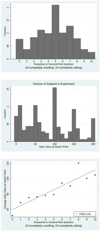
general risk question is very similar. While the mean (median) value in the experiment is 4.76 (5), it is 4.42 (5) for the people who are interviewed in the SOEP. In addition the answers to the general risk question are almost identically distributed (compare Figure 1 and Figure 5, upper panel).18
The middle panel of Figure 5 shows a histogram of subjects’ choices in the experi-ment. About 78 percent of the participants are risk averse, in the sense that they prefer not to play the lottery, which has an expected value of 150 Euros, when offered a safe payment smaller than 150 Euros. About 13 percent are arguably risk neutral: 9 percent prefer a safe payment of 150 Euros to the lottery, but play the lottery at smaller alternative options, and 4 percent play the lottery when offered a safe payment equal to the expected value of the lottery but do not play the lottery when the safe payment exceeds the ex-pected value of the lottery. About 9 percent of the subjects reveal risk loving preferences, preferring the lottery to safe amounts above 150 Euros.
Our main interest in this section is whether survey data can predict actual risk taking behavior in the lottery experiment. In other words, we want to study whether subjects who indicated a greater willingness to take risks in the general risk question also show a greater willingness to take risks in the lottery experiment. A first indication that this is indeed the case is given by the lower panel of Figure 5. The figure shows a scatter plot where the average certainty equivalents observed in the experiment, i.e. the average of the smallest safe options that the corresponding subjects preferred over the lottery, are plotted against the survey answers. The figure reveals a clearly positive relation.19 To test the predictive power of the general risk question more rigorously, we ran the regressions reported in the lower panel of Table 2. In the first model, we simply regress answers given to the general risk question on the value of the safe option at the switching point. The general risk coefficient is positive and significant at any conventional level indicating that the answers given in the survey do predict actual risk taking behavior. To check robustness, we add controls in Columns 2 and 3, which are essentially the same as the controls in Table 1. In Column 2 we add gender, age, and height as explanatory variables. In Column 3, we control for many additional individual characteristics, as in TableA.1 in 18
A Kolmogorov-Smirnov-test does not reject the null hypothesis that the answers to the survey risk questions in the two samples have the same distribution.
19
For the calculation of the average value of the switching point we set the value of the safe option equal to 200 for the 31 participants who always prefer the lottery.
the appendix. The general risk coefficient becomes somewhat smaller but stays significant at the one percent level. In sum, the answers to the general risk attitude question predict actual behavior in the lottery quite well, confirming the behavioral relevance of this survey measure.
5
A Lottery Measure of Risk Preference: The Hypothetical
Investment Question
It is important to compare our findings based on the general risk measure to a more standard lottery measure. In this section we return to the issues of heterogeneity and exogenous determinants of risk attitudes, but use investment choices in the hypothetical investment scenario as the measure of willingness to take risks. We also show how, under specific assumptions, responses to the investment question can be used to recover a pa-rameter value describing the curvature of the individual’s utility function, corresponding to the theoretical concept of risk preference in expected utility theory.
5.1 Risk Attitudes in a Hypothetical Lottery
Respondents in the SOEP were asked how much of 100,000 Euros in lottery winnings they would choose to invest, in a hypothetical asset promising, with equal probability, to either halve or double their investment in two years time. The question offered respondents six possible investment amounts: 0, 20,000, 40,000, 60,000, 80,000, or 100,000 Euros. Importantly, these stakes are large enough to have a potentially significant impact on lifetime utility; 100,000 Euros is roughly five times the average annual net individual income of respondents in the sample (21,524 Euros).
Figure 6 shows the distribution of responses to the investment question in the sample. The histogram indicates that roughly 60 percent of the survey respondents chose not to invest in the hypothetical asset.20 The remaining 40 percent did choose to invest, with substantial variation in terms of the amount, although the fraction of individuals investing decreases as the investment amount becomes larger. Thus, similar to the general risk question, the hypothetical investment measure reveals substantial heterogeneity. In fact,
20A similar share of the sample, roughly 68 percent, chose a value less than 6 on the general risk scale and
the correlation between investment choices and responses to the general risk question is fairly strong, about 0.26, indicating a significant overlap in terms of what these questions measure.
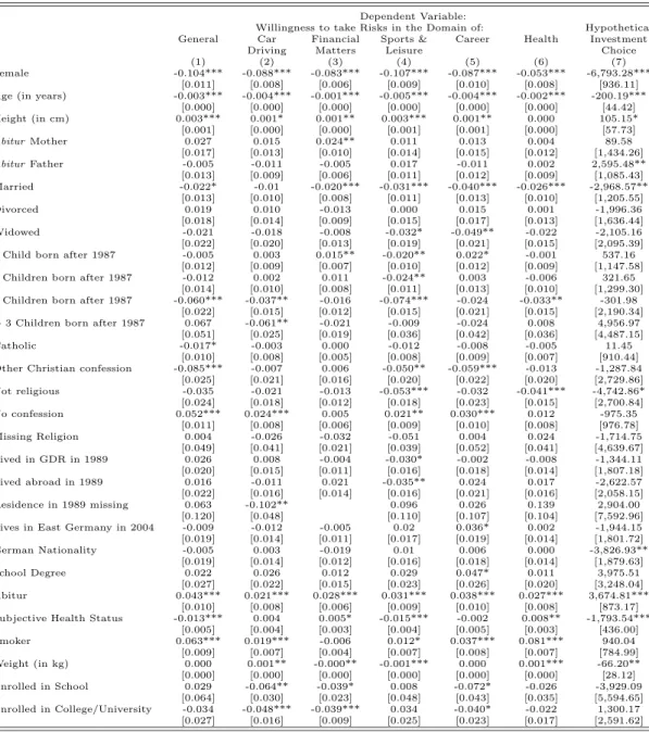
In order to explore the determinants of individual differences in willingness to invest, we regress the amount invested in the lottery on exogenous factors and other controls. The resulting coefficient estimates are presented in Table 3. We do not adopt a binary measure for the dependent variable, as we did in the case of the general risk question, because it is more difficult to choose a sensible division of the scale. Also, we want our coefficient estimates to reflect the impact of exogenous factors on the amount of Euros invested.21
We use an estimation procedure that accounts for the fact that the dependent variable is measured in intervals, and hence is left and right censored. A negative coefficient indicates a lower willingness to invest and therefore a lower willingness to take risks.
In Table 3, the right-hand side variables for Columns (1) to (9) correspond exactly to those used in the analysis of the general risk question, in Table 1. The baseline results, without income, wealth and additional controls, are shown in Column (1). The marginal effects indicate that women invest about 6000 Euros less in the risky asset than men. Each year of age tends to reduce the investment by about 350 Euros.22 Finally, each centimeter of height leads to about 200 Euros higher investment in the risky asset. These effects are substantial, and they are all highly significant. They are also qualitatively similar to the findings based on the general risk question. In contrast, the results for parental education are somewhat different. While father’s education exhibits a large and highly significant positive effect on willingness to invest, mother’s education has no explanatory power for investment choices. Adding additional controls in Columns (2) to (9) leaves these results qualitatively unchanged.
These findings are noteworthy given that the hypothetical investment question in-volves a relatively concrete context, in terms of a legitimate investment opportunity. For instance, the gender effect we find contrasts with Schubert et al. (1999), who conduct lottery experiments with undergraduates, and find that gender differences become in-21
As a robustness check, we estimated the regressions using a binary measure as the dependent variable, indicating whether an individual invests a positive amount. We found very similar results in this case.
22
A specification with three splines with knots at 30 and 60 years reveals that age has no significant effect on investment for the youngest age category, significant and large effects of 300 and 640 Euros per year of age, respectively, for the two older age categories.
significant when lotteries are framed as investment opportunities. In Section 6 we explore the issue of context in more detail.
5.2 Implied Coefficients of Risk Aversion
Responses to the hypothetical investment question provide cardinal information on in-dividuals’ relative willingness to take risks, i.e., differences in investment choices can be measured in Euros. Assuming the existence of a canonical utility function, this informa-tion can be combined with a measure of individual wealth and converted into a measure of the degree of curvature of the utility function.
Assume that the individual’s utility function is characterized by constant relative risk aversion, so that utility has the form u(x) = x11−−γγ, which is a function of a wealth endowment (or consumption possibilities)x. The CRRA parameterγdescribes the degree of relative risk aversion for an individual: the individual is risk loving ifγ <0, risk neutral ifγ = 0, and risk averse ifγ >0.23 Using an individual’s investment choice, and additional survey information on the individual’s wealth level before the investment, it is possible to compute an interval for the individual’s CRRA parameter.24 Intuitively, the choice of a given investment implies that the expected utility from this option must be greater than or equal to the utility derived from any other option, in particular the next largest, and next smallest possible investment choice. Expressing these two conditions in terms of the individual’s utility function, and substituting the wealth level as an argument, it is possible to solve for upper and lower bound values forγ >0 (see Barskyet al., 1997, and Holt and Laury, 2002, for a similar approach). Given that the stakes in our hypothetical investment scenario are large enough to be meaningful in terms of lifetime consumption, and given that the calculation incorporates information on current wealth, the resulting parameter ranges can be interpreted as referring to the curvature of the lifetime utility function.25
23Note that lim
γ→1u(x) = lnx.
24Note that heterogeneity in the initial wealth level implies that individuals with the same answer to the
investment question may have different CRRA intervals.
25
Unlike Barskyet al.(1997) or Holt and Laury (2002), our calculation takes into account current wealth
levels (including the 100,000 Euros of hypothetical endowment). Guiso and Paiella (2005) take a differ-ent approach altogether. They derive a point estimate for the degree of absolute risk aversion using a local approximation of the utility function around imputed lifetime wealth. As noted by the authors, this approximation is only reasonable for an investment with relatively small stakes, like the one in-cluded in their survey. The much larger stakes in our hypothetical investment question make such an
The top panel of Figure 7 shows the distribution of interval mid-points in the sample. The figure excludes individuals investing 0 Euros or 100,000 Euros. Individuals who invest nothing are clearly risk averse, but the interval for their CRRA coefficient cannot be displayed in the graph because it is not bounded from above. Conversely, individuals who invest 100,000 Euros are relatively risk-seeking, but the lower bound for their interval cannot be determined.26 In the literature, values for the CRRA coefficient between 1 and
5 are typically perceived as reasonable, and values above 10 are considered unrealistic (for discussions on this point see Kocherlakota, 1996; Cecchettiet al., 2000; Gollier, 2001, p. 31). The conditional distribution in Figure 7 is consistent with this perception: the bulk of the mass in the distribution is located between 1 and 10. There is, however, a non-negligible mass of midpoints in the range of higher values, up to about 20.27
The middle panel of Figure 7 provides a different perspective on the data. It shows the cumulative distributions of lower and upper bounds for γ in the population (the cu-mulative for upper bounds is the lower line in the figure), excluding individuals who invest 0 or 100,000 Euros. For any given value ofγ on the horizontal axis, the vertical difference between the two curves gives the fraction of individuals with an interval containing that value of γ. The figure confirms that most intervals contain a γ between 1 and 10. The bottom panel in the figure shows the cumulative distributions for upper and lower bounds ofγ using the whole sample including non-investors and individuals investing the the full amount of 100,000 Euros. Since γ cannot be bounded from a above for the 61 percent of individuals investing zero, the cumulative distribution converges to 39 percent in the range of values for γ on the horizontal axis. Likewise, γ cannot be bounded from below for those who invest the full amount.
In principle, it is also possible to construct a distribution of CRRA coefficients using the lottery choices in our field experiment, described in Section 4. An important caveat, approximation inadvisable. Indeed, computations of CRRA coefficients for the SOEP sample using a local approximation of the utility function yield exceedingly high levels of risk aversion compared to the
interval approach depicted in Figure 7. Donkerset al.(2001) also calculate preference parameters using
lottery responses, but in a model derived from cumulative prospect theory rather than in the expected utility framework.
26Thus the investment question does not allow us to say whether individuals investing 100,00 are mildly
risk averse, with aγclose to 0, or whether they are actually risk loving, withγ <0.
27
This is potentially explained by measurement error in wealth levels, the neglect of incomes in the computation, or the underestimation of the true expected value of the lottery because of probability-weighting.
however, is that the lottery measure in the field experiment is not as well-suited for this pur-pose as the hypothetical lottery in the SOEP, because the stakes are relatively small (300 Euros). As shown by Rabin (2000), the curvature of the lifetime utility function should be approximately linear for stakes in this range, assuming a typical wealth level.28 In order
to avoid inferring extreme parameter values from such lottery choices, it is typically nec-essary to assume an initial wealth level of zero, or equivalently that individuals ”ignore” current wealth when making their decision (Wattet al., 2002). Making this assumption, as is done in, e.g., Holt and Laury (2002), indifference between a lottery involving 300 Euros or 0 Euros with probabilityp= 0.5, and a safe option ofy, impliesp·3001−1γ−γ = y11−−γγ. Therefore, γ = 1−lny−lnln 300p , which gives us bounds for the interval containing γ. It is then possible to assign an interval to each of the switching points observed in the field experiment, displayed in the middle panel of Figure 5. In particular, the pairings of each switching point with the midpoint of the associated CRRA interval, (y, γ), are as follows: (0,∞), (10,0.796), (20,0.744), (30,0.699), (40,0.656), (50,0.613), (60,0.569), (70,0.524), (80,0.476), (90,0.424), (100,0.369), (110,0.309), (120,0.244), (130,0.171), (140,0.091), (150,0), (160,−0.103), (170,−0.220), (180,−0.357), (190,−0.518). Thus, looking at Fig-ure 5, roughly 10 percent of individuals in the field experiment have a CRRA interval midpoint of 0.796, 10 percent have a midpoint of 0.613, and so on.
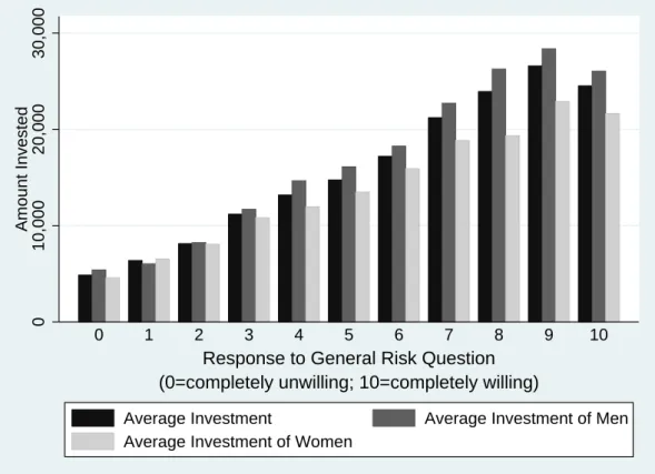
It would be valuable to be able to interpret responses to the general risk question in terms of coefficient intervals. In this case researchers could take advantage of the relatively simple and easy-to-ask format of the general risk question without sacrificing the ability to gather information on preference parameters. We conclude this section by showing how the SOEP data can be used to construct the necessary mapping. Figure 8 shows the average amount invested in the risky asset for each possible answer to the general risk question, among all individuals and also separately for men and women. This is the information necessary for the first step in imputing ranges for the CRRA coefficient based on responses to the general risk question. To see how the imputation works, suppose an individual reports a willingness to take risks of 4 on the general risk scale. According to the figure, individuals with such a response invest on average 13,184 Euros in the hypothetical investment. Combining this information with data on the individual’s wealth endowment, 28
In fact, if we use the information on wealth and income included in the field experiment and calculate CRRA intervals as in the SOEP, we obtain extreme coefficient estimates (available upon request) by this procedure.
say 25,000 Euros, straightforward computation leads to a CRRA coefficient for this person of around 4.5. Alternatively, suppose a man with a wealth endowment of 100,000 Euros reports a willingness to take risks of 7. On average, he would invest 22,716 Euros in the risky asset, implying a CRRA coefficient of about 4.1. Finally, the CRRA coefficient of a woman endowed with 30,000 Euros of wealth, choosing a value of 2 on the general risk scale, is predicted to be around around 7.55, using the information that women reporting a value of 2 invest on average 8,064 Euros into the hypothetical asset. The type of mapping illustrated in Figure 8 is thus a potentially useful tool, adding to the value of the general risk question for researchers who are interested in CRRA coefficients.
In summary, results on heterogeneity and determinants using the hypothetical lot-tery question are similar to those obtained using the general risk question. Given that the investment scenario holds risk perceptions constant, however, these effects are more clearly attributable to differences in risk preference.29 These findings are also noteworthy because they persist even though the question incorporates concrete context, in the form of an investment opportunity. The estimates for CRRA parameters provide information about the distribution of risk preferences in the population, assuming that a CRRA util-ity function exists for all individuals. The mapping provided at the end of the section potentially adds to the value of the general risk question.
6
Risk Attitudes and Context
This section investigates the role of context in shaping risk attitudes. In economics it is standard to assume the existence of a single risk trait governing risk taking in all contexts. In line with this assumption, economists typically use a lottery measure framed as a financial decision as an indicator of risk attitudes in all other contexts. By contrast, there is considerable controversy on this point in psychology. Based on laboratory experiments in which self-reported risk taking is only weakly correlated across different contexts, some studies conclude that a stable risk trait does not exist at all (see Slovic, 1972a and 1972b for a review). We contribute to this discussion in several ways. First, we study the impact 29
Note, however, previous evidence on gender differences in probability-weighting. For example, Fehr-Dudaet al. (2004) conduct an experiment on risky choice, involving explicit stakes and probabilities, and find evidence for a gender difference in willingness to take risks that is due to different perceptions
of how “large” or “small” the probabilities are. Donkerset al.(2001) also find evidence that individual
of context on a much larger scale using a representative sample. Second, we measure the correlation of willingness to take risks across the different contexts identified in the SOEP: general, car driving, financial matters, sports and leisure, health, and career. Little or no correlation would provide evidence against the standard assumption; a strong correlation would suggest the existence of a stable risk trait. We then explore the determinants of willingness to take risks in specific contexts. Evidence that the same factors determine risk attitudes across contexts, in a similar way, would also lend support to the notion of a stable risk trait.
6.1 Correlation Across Domains
The first section of Table 4 reports mean responses for each domain-specific question and the general risk question.30 Context appears to matter for self-reported willingness to take risks. The ranking in willingness to take risks, from greatest to least, is as follows: general, career, sports and leisure, car driving, health, and financial matters. The same ranking holds for both men and women. Notably, women are less willing to take risks than men in every domain.
The next section in the table shows simple pairwise correlations between individuals’ risk attitudes in different contexts. Risk attitudes are not perfectly correlated across domains, but the correlations are large, typically in the neighborhood of 0.5, and all are highly significant. Another way of assessing the stability of risk attitudes is to check what fraction of individuals is relatively willing to take risks (choose a value greater than 5) for all of the six different measures. It turns out that 51 percent of individuals are relatively willing to take risks in all six domains, by this definition, and more than one third are relatively willing in at least five domains. The strong correlation across contexts, and the stability of an individual’s disposition towards risk across domains, strongly suggest the presence of a stable, underlying risk trait. The consistency across domains is not perfect, and could indicate some malleability of risk preferences, but it seems more likely that this reflects variation in the risk perception component of the measures across domains, e.g., a tendency for most people to view the typical risk in car driving as more dangerous than 30
The different numbers of observations across domains reflects different non-response rates. These dif-ferences may arise because individuals feel certain questions do not apply to them, e.g., a 90-year-old without a driver’s license is free to leave blank the question about taking risks while driving a car.
the typical risk in sports and thus to state a relatively lower willingness to take risks in car driving.
The lower portion of Table 4 reports similar statistics, but using binary versions of each question. These are constructed in the same way as the binary version of the general risk question used in Section 3: for each domain, the indicator is equal to 1 for responses higher than 5 on the question scale and 0 otherwise. The means of these binary risk measures can be interpreted as the fraction of individuals in each domain who are relatively willing to take risks. The correlations across domains using the binary measures range from 0.24 to 0.47 and are highly significant.
Principal components analysis using the general risk question and the five domain-specific questions tells a similar story. About 60 percent of the variation in individual risk attitudes is explained by one principal component, consistent with the existence of a single underlying trait determining willingness to take risks.31 Nevertheless, each of the other five components explains at least five percent of the variation, which again suggests that there is some additional content captured by the domain-specific measures.
6.2 Determinants of Risk Attitudes in Different Domains
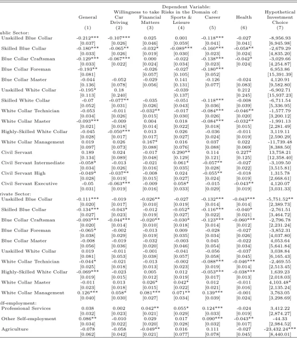
Table 5 explores the determinants of individual risk attitudes in each of the five domains identified in the SOEP. For ease of comparison, the first column reports results for the general risk domain, shown previously in Table 1. The remaining columns report marginal effect estimates from Probit regressions, where the dependent variables are the binary versions of each domain-specific question.32 These binary measures are the same as the ones reported in the lower section of Table 4 above, with a 1 indicating that an individual is relatively willing to take risks (i.e., chooses a value greater than 5 on the response scale). From Columns (2) to (9) it is apparent that the impact of the exogenous factors is, for the most part, qualitatively similar across contexts. Women are significantly less willing to take risks than men in all domains.33 Gender differences are most pronounced 31
The eigenvalue associated with this component equals 3.61 while the eigenvalues associated with all other components are smaller than 0.57. When only one component is retained, none of the off-diagonal
elements of the residual correlation matrix exceeds|0.11|.
32
The results are robust if we instead run linear probability models (OLS) or ordered probits, using the 11-point scale measures rather than binary measures as dependent variables.
33A Oaxaca-Blinder decomposition reveals that across domains, more than 60 to 70 percent of this