DYNAMIC STRUCTURAL MODELS OF RETIREMENT AND DISABILITY

DYNAMIC STRUCTURAL MODELS OF RETIREMENT AND DISABILITY

John Rust, University of Maryland and NBER Moshe Buchinsky, UCLA and NBER Hugo Benítez-Silva, SUNY--Stony Brook

February 2003

SUMMARY

We propose to use all available waves of the Health and Retirement Survey (HRS) and AHEAD Survey to estimate a comprehensive dynamic programming (DP) model of behavior at the end of the life cycle that provides a detailed treatment of the Social Security Administration's (SSA) Old Age and Survivors (OASI), Supplemental Security Income (SSI) and Disability Insurance (DI) programs. Major changes to these

programs are being contemplated. Yet, we currently lack a unified model of social insurance at the end of the life cycle that can help us evaluate the behavioral and distributional impacts of these policies. Particular attention is paid to developing, estimating, and testing a multi-stage dynamic programming (DP) model of the SSI and DI application, appeal, and award process, for (possibly) heterogeneous agents.

We are developing a tractable empirical model that captures an individual's decisions regarding (1) labor supply and retirement (2) application for OA, DI and SSI benefits, and (3) consumption and savings.

The resulting model will allow us to derive predictions of the behavioral and welfare implications of policy changes. While there is a large literature using reduced-form and static structural models that has investigated some of these issues, it suffers from two major shortcomings. First, reduced-form models cannot be used for welfare analysis or to predict behavior responses to policy changes. Second, static structural models do not accurately reflect the level of complexity and uncertainty facing individual decision makers, nor do they capture the important dynamic elements of the decision processes. The DP model we are developing will circumvent these shortcomings, providing a tractable framework for analyzing individual behavior and well-being, and forecasting their response to a wide range of policy changes.

Our model could provide new insights into a number of puzzling aspects about disability in the U.S. One puzzle is to determine the factors responsible for the pronounced swings in DI incidence rates in recent years. Another puzzle is to determine why the fraction of Americans receiving SSI and DI benefits continues to increase despite overwhelming epidemiological evidence of steady improvements in various objective indicators of health status. The SSA is currently contemplating significant changes to the disability award process, in order to reduce delays, and reduce large unexplained state-level differences in award rates.

We will use detailed health and functional status indicators from the HRS to evaluate whether or not there are alternative screening rules that can reduce the level of classification errors in the DI award process. Our estimated DP model will produce detailed predictions of the behavioral and welfare effects of changes in benefit levels, delays, the probability of being awarded benefits, and the probability that a DI beneficiary will be audited. This framework will allow us to develop methodologies for characterizing efficient policies, i.e., those that minimize the expected discounted cost of providing a stream of social insurance benefits subject to the constraint that individuals' expected discounted utilities are at least as high as under the status quo.

1. INTRODUCTION AND SPECIFIC AIMS

The life-cycle model has been a cornerstone of economics for over 50 years, yet surprisingly only within the last few years have economists begun to consider how to estimate and test it. Although economists such as Bernheim (1993, 1994, 1995, 1996, and 1997) have claimed that observed behavior is inconsistent with the predictions of the life-cycle model since “These studies consistently find that baby boomers are saving at 33 to 38 percent of the rate required to cover their expected costs of retirement.” (Bernheim 1997, p. 43). We argue that most economists do not really understand the implications and richness of the full life cycle model because they have been unable to solve realistic versions of it. Instead they have relied on limited, often incorrect intuitions obtained from overly simplified deterministic/stochastic specifications that yield analytic solutions. Virtually all empirical work has avoided solving the full life-cycle model by

estimating and testing essentially static partial characterizations of optimality such as the Euler necessary condition that implies that (for interior solutions) the marginal rate of substitution between consumption and labor supply equals the current wage rate.

Recently, the advent of improved algorithms and computer hardware have allowed economists to solve more realistic specifications of the life cycle model, resulting in a much deeper understanding of its

implications and the realization that versions of the life-cycle model might be capable of explaining observed behavior. For example, Engen, Gale, and Uccello (1999) solved and simulated a calibrated version of the life-cycle model and compared the predicted levels of saving and wealth accumulation to levels observed in the Health and Retirement Survey (HRS) and the Survey of Consumer Finances. They conclude that, contrary to Bernheim, observed saving behavior appears to be adequate in the sense that the predicted levels of saving and wealth accumulation in their calibrated life-cycle model appear to be roughly consistent with observed levels. They find that “Because of the uncertainty of earnings, the model generates a distribution of optimal wealth-earnings ratios among households that are observationally equivalent. This distribution implies that some households that have very low wealth-earnings ratios are nonetheless saving optimally for retirement.” (p. 141).

A limitation of Engen et al. (1999) is that labor earnings are treated as an exogenous stochastic process. In reality it is mostly an endogenous process resulting from an individual's labor supply decision. As we show below, once we model labor supply and consumption jointly, the predictions of the life-cycle become much richer. Surprisingly low levels of wealth accumulation can be optimal if an individual expects to retire later than “normal”, an expectation that surveys have found to be common among baby boomers. The close interaction between retirement expectations and preretirement savings was noted as far back as Feldstein (1974), but to our knowledge the magnitude of the effect of retirement age expectations on the level of preretirement savings has not been empirically demonstrated. It is one of the questions we will attempt to answer in this research.

Finally, it has also been known that low levels of saving can be optimal in the presence of Social Security and other forms of social insurance. For example Hubbard, Skinner and Zeldes (1995) showed that it can be optimal for individuals with the lowest earnings capacities to hold almost no wealth when asset testing is a precondition for the receipt of Medicaid and welfare benefits. All these considerations suggest that a considerably richer version of the life-cycle model --- with joint treatment of consumption and labor supply and a realistic treatment of social insurance institutions --- will be necessary before we can judge whether or not individuals are behaving optimally and in accordance with the predictions of the life-cycle model.

To date, most empirical work on the life-cycle model has been based on relatively informal comparisons of observed behavior with the simulated behavior from calibrated versions of the life-cycle model.

Calibration style methods specify values for the parameters of the model, partly because it is too hard to write down a formal likelihood function for the model, and partly because it is too computationally

demanding to repeatedly resolve the life-cycle model in a formal search for best fitting values of the model's unknown parameters.

Recently pioneering work by French (2001), building on previous methods developed by Rust and Phelan (1997), has provided the first econometric estimates of life-cycle models where consumption and labor supply are jointly endogenous and social insurance institutions are carefully modeled (although econometric methods for estimating the life-cycle model can be traced as far back as Heckman 1974, Heckman's early work was based on deterministic models of the life-cycle and abstracted from social insurance institutions). We are not aware of any readily available econometric methods that economists can use to compute, simulate, estimate, and test the life-cycle model that incorporates a continuous decision over consumption and a discrete or continuous decision over labor supply. The purpose of this proposal is to develop new, computationally efficient methods for doing this, and to apply these techniques to the study of behavior in the last half of the life-cycle, paying particularly close attention to how consumption and labor supply behavior are affected by social insurance, pension, and private insurance institutions.

Specifically, we propose to develop a unified empirical model of social insurance at the end of the life-cycle using data from the HRS and the AHEAD Survey. Our model will include a detailed treatment of the following components of the U.S. Social Security system: (1) Old Age and Survivors Insurance (OASI); (2) Disability Insurance (DI) and Supplemental Security Income (SSI) benefits; (3) Medicare and Medicaid, and (4) Unemployment Insurance (UI). We will also pay close attention to modeling taxes including: (1) the Federal income tax and Earned Income Tax Credit (EITC); (2) the estate tax; and (3) state and local income taxes, sales taxes, and property taxes. The result will be a model that will enable us to analyze a wide variety of tax and transfer policies, particularly those associated with Social Security reform.

Because of the aging of the U.S. society, the Social Security program is not in long run actuarial balance. Eventually, Congress will have to decide on whether significant tax increases, benefit cuts, or even more drastic changes, will be needed. A number of important changes will begin to take effect in coming years as a result of the 1983 Social Security amendments, which was intended to create incentives for delayed retirement in order to restore the long run balance in the OASI program. In addition to increasing contribution rates, the 1983 amendments increased the normal retirement age (NRA) from 65 to 67, increased the delayed retirement credit (DRC) from 1% to 8%, and decreased the “retirement test” tax on post-retirement earnings, first from 50% to 33%, and in the last year of the Clinton Administration, all the way to 0% for people over 65. In recent years much more radical changes to the Social Security program have been proposed, including the introduction of individual accounts, and major changes in the way the DI program is administered. These, and other policy measures, can be examined in our framework.

Our research will place particularly high priority on developing a fully dynamic model of the SSI and DI programs. We do this in part because the DI program has never been previously modeled in a fully dynamic context, and also because the DI program provides a unique opportunity to subject the estimated life-cycle model to a strong experimental test. The Project Leader, John Rust, has been appointed as an advisor to the Social Security Administration (SSA) to assist in the implementation of a large scale “demonstration project” mandated under the 1999 Ticket to Work Act and Work Incentives Improvement Act (TWWIIA). The demonstration project will essentially be a huge controlled experiment in which certain DI recipients will be randomly assigned alternative benefit formulae. A particular alternative was specified in the TWWIIA Act: it is known internally at the SSA as the “2 for 1 benefit offset”. Under the current rules, a DI recipient who returns to work and earns more than a set-aside amount known as the substantial gainful activity level (SGA) (currently equal to $700 per month), loses all of her DI benefits if she continues to earn more than the SGA level beyond a 9 month trial work period. The 2 for 1 offset proposal would reduce the effective 100% tax on earnings in excess of the SGA to 50%. The SSA also has the authority to change the SGA level, i.e., to change the disregard level at which this 50% tax kicks in. The demonstration project

provides a unique opportunity to put the life-cycle model to a rigorous test: we propose to estimate a life-cycle model using the HRS and AHEAD data and use the estimated model to generate predictions of the behavioral response of the DI recipients who are assigned the “treatment” in the TWWIIA demonstration project. If our life-cycle model is able to accurately predict the “actual response” of the DI recipients who are randomly assigned the 2 for 1 offset, it will have much more credibility for use in a variety of other important policy forecasting tasks confronting the SSA in coming years.

Ever since the work of Lalonde (1986) and Lalonde and Maynard (1987) there has been some skepticism about the reliability of complicated econometric models for use in policy forecasting. The skepticism is part of the reason why the Congress has mandated the use of experimental methods for policy evaluation. However, Heckman, Hotz and Dabos (1987) pointed out a number of severe limitations of the experimental approach to policy evaluation, not the least of which are the huge costs and delays involved in implementing large scale social experiments. An example of a serious limitation that the SSA is confronting in its mandate to carry out the TWWIIA project is related to a phenomenon known as the induced entry effect. This effect arises because the 2 for 1 offset proposal amounts to a liberalization of the DI benefit rules: more benefits will be paid to DI recipients if the 2 for 1 offset plan is in place if they should choose to return to work. Ex ante, a more liberal DI program should induce additional entry by individuals who are

considering whether or not to apply to the program. A number of initial intelligent “guesstimates” produced by the SSA Office of the Actuary have suggested that the 2 for 1 offset policy could significantly increase the cost of the DI program because the additional benefits paid to new recipients due to induced entry would exceed the reduction in benefits to DI recipients who would leave the roles as a consequence of “induced exit”. Although the change in the probability of applying for DI benefits is thought to be very small, a small increase in the probability of entry spread out over a large population of potential entrants can result in a substantial increase in DI roles and costs in the long run. For similar reasons, statisticians advising the SSA have estimated that it would take extremely large sample sizes --- on the order of hundreds of thousands or even millions of subjects --- to generate statistically reliable estimates of the induced entry effect. Due to the huge cost of such a study, it is very unlikely that the SSA will be able to use experimental methods to measure the full budgetary impact of the 2 for 1 offset policy. This is a case where a credible behavioral life-cycle model may be one of the only ways for the SSA to provide predictions of the total impact of the policy change.

Our life-cycle model will also be useful for analyzing a number of other changes to the DI program that have recently been contemplated. Many of the proposed changes resulted from the huge increases in

processing delays and backlogs following the rapid growth in applications and appeals during the early 1990s. As part of its “Disability Process Redesign” (DPR) plan, the SSA has considered implementing major changes in the multi stage application and appeal process in order to reduce the long delays between an initial application and an ultimate award, including possibly multiple levels of appeals if the initial application is rejected by one of the 54 state-run disability determination services (DDS). The SSA is also considering the use of standardized functional impairment indices in order to reduce the large state-to-state variations in award rates. All of these proposed policy changes will have significant effects on the structure of the Social Security program that cannot be accurately predicted and examined using reduced-form methods that are only able to estimate behavioral relationships that hold under the status quo but which may not continue to be valid after a significant policy change. Currently, there is no unified behavioral model that the SSA can rely on to forecast the behavioral and welfare implications of any of these policy changes. The only comprehensive way to deal with these multitude of questions is by modeling explicitly the decision processes by both the individuals and the SSA, under realistic assumptions governing their behavior.

Fortunately, in recent years increasingly realistic dynamic structural models have been formulated and estimated. These models include Rust and Phelan (1997), which estimated a detailed dynamic programming

model of the OASI and Medicare program. In contrast to reduced-form papers in the literature, the innovation of their work is that they showed that a number of previously puzzling aspects of retirement behavior are simply artifacts of particular details of the Social Security rules. In particular, they showed that OASI and Medicare benefits have complex interacting incentive effects, and that seriously misleading policy conclusions can be drawn from studies that attempt to study OASI and Medicare in isolation from each other. The Rust-Phelan model was able to provide coherent economic explanations for a wide variety of

phenomena observed in the data, including the pronounced peaks in the distribution of retirement ages at 62 and 65. These results illustrate the potential payoffs to developing an integrated dynamic model of social insurance at the end of the life-cycle. We will relax some of the key limitations of the Rust-Phelan model (particularly their assumption that consumption equals income) and use this more general life-cycle model to analyze a number of important policy-related questions and issues including:

1) Why does the fraction of Americans on the DI and SSI roles continue to increase when

epidemiological studies find that health of older Americans has improved over time? 2) What is the relative importance of changes in award rates, unemployment rates, welfare reform, and social factors in the large swings in DI incidence rates in recent years? 3) What impact do delays in the DI award process have on incentives to apply or appeal? Will proposals to speed up this process increase the number of applications and awards? 4) How would retirement incentives and individual welfare be affected by an introduction of “individual accounts” similar to President Bush's proposed plan? 5) Will the 1983 Social Security

Amendments, particularly the increase in the NRA and DRC, cause individuals to significantly delay the age at which they apply for OA benefits? How would individuals' be affected if the Medicare eligibility age (MEA) were also increased? 6) Will the increase in the normal retirement age (NRA) increase the incentive to apply for SSI and DI benefits prior to the NRA? If so, to what extent will any reduction in the costs of the OA program due to the increased NRA be offset by an increase in the cost of the SSI/DI program?

Our model can also address a wide range of policy issues connected with taxation, such as predicting the impact of the recent changes in the estate tax on savings and bequest decisions. However, we will devote most of our attention to modeling the dynamics of disability, mortality, and health, and the factors

influencing decisions to apply for SSI and DI benefits, since these are relatively volatile programs that have grown at unsustainable rates in recent years.

2. BACKGROUND AND SIGNIFICANCE

There is a large empirical literature studying the factors affecting DI applications and awards, and a somewhat smaller literature on the SSI program. This literature, (e.g. Rupp and Stapleton, 1996, or Stapleton et al. 1994) has identified a number of important factors: (1) benefit levels; (2) program leniency as measured by award probabilities and audit rates; (3) strength of the demand for labor; (4) the availability of alternative sources of support; and (5) social attitudes and stigma associated with receiving DI benefits. However, the relative importance of these factors is still not well understood, hampering the SSA's ability to do policy analysis and short and long term forecasting. Figures 1 and 2 illustrate some of the key historical and forecasted trends in the DI program.

Figure 1 summarizes the historical and projected trends in the size and cost of the DI program, measured by the DI prevalence rate and by the ratio of DI expenditures to GDP. The right hand side of Figure 1 shows a rapid rise in the cost of the DI program since its inception in 1956 until the mid 1970s, interrupted only by a decrease in the cost of the program during a period of retrenchment from 1977 to 1990, and a decrease during the economic boom of recent years. The Actuary forecasts continued growth in the program over the next 75 years, topping out at roughly 0.9% of GDP by 2075. The left hand panel of Figure 1 plots historical and projected prevalence of DI over the period 1988 to 2075. We see that prevalence rates have increased steadily over the period 1988 to 1996, pausing briefly in 1997 and 1998. The Actuary forecasts a particularly

rapid increase in DI prevalence until 2030, by which time most of the baby boom generation will have reached normal retirement age. Thereafter prevalence continues to grow at a more moderate rate reaching 7% of the insured population by 2075. The “adjusted” prevalence curve is based on the assumption that the age distribution of the U.S. remains at its 1998 values. While the unadjusted prevalence rates increase from 4% to 7% between 1999 and 2075, the adjusted prevalence rate increases to only 5%. Thus, population aging accounts for only about one third of the projected increase in prevalence of DI in the next 75 years.

Figure 1: Historical and Forecasted Growth in SSDI Roles and Costs

Figure 2 illustrates some of the historical volatility in application and award rates. The left hand panel plots the trend in the “crude” acceptance rate---the ratio of the number of new DI awards to the total number of applications and appeals files in a given year. The right hand panel plots the ratio of DI applications and awards to the DI insured population. The award rate reached its lowest level in 1982 during the Reagan Administration, during a clamp-down on the DI and SSI programs. There was a large increase in audits, also known as “Continuing Disability Reviews” (CDR), during this period. The combined effect was to strongly discourage individuals from applying for DI benefits. On the other hand, DI applications and awards peak in 1974 due to several factors: (1) a recession in the early 1970s; (2) a rapid increase in benefit levels due to an error in the 1972 Social Security amendments which resulted in an inadvertent double indexing of Social Security benefits to inflation; and (3) a lenient policy towards DI applicants. SSI was also introduced in 1974, so the public may have actually perceived the SSA as encouraging applicants, reducing perceived “hassle costs” to applying for DI or the stigma associated with receiving benefits. DI application rates began growing rapidly again in the early 1990s following a sustained period of growth in award rates. The causes of this rapid burst of growth are not fully understood, but high unemployment rates in the early 1990s, and a cutback in state General Assistance (GA) programs are thought to be important contributing factors. The passage of the Americans with Disabilities Act in 1990 was designed to force employers to accommodate workers with disabilities and thus reduce the incidence and prevalence of individuals receiving DI benefits.

Figure 2: History of SSDI Application and Award Rates, Roles, and Costs

Application rates declined equally quickly after 1993. This was also the peak year for enrollments in the AFDC program, and a period of high social stigma towards welfare recipients may have been one of the most important factors motivating the tough 1996 Welfare Reform Act. While part of the decline in application rates might be ascribed to an increase in real or perceived stigma towards AFDC and SSI recipients, the years after 1993 have also constituted the longest peacetime economic boom in recorded history. Only within a structural model can one make an attempt to disentangle the relative contributions of these two possible explanations.

The paradox that DI prevalence rates have grown while the objective health status of Americans has improved, suggests that the concept of “disability” used by the SSA is not based on an absolute objectively determinable measure of physical status, but is rather more akin to a socially defined concept whose absolute standards may change over time with changes in the political, social, and technological climate. Clearly, the nature of physical/mental conditions that are regarded as disabling is very different in today's “information economy” than they were in an industrial/agrarian economy early in the century. It is not surprising therefore that the SSA documents significant changes in the distribution of impairments that are listed as the primary reasons being awarded DI benefits.1

We believe that the way the SSA administers the DI award process can help to create a “social standard” that has a powerful impact on the public's perception of the thresholds for mental and physical impairments that are sufficiently severe to constitute “disability”. Indeed, we have shown (see Benítez-Silva et al. 2001) that self-reported disability status is an unbiased indicator of the SSA's ultimate award decision. This finding suggests the possibility that tightening or loosening of DI award rates may have a double effect. Its direct effect is on the individuals' incentives for applying for benefits since it affects their chances of success. The indirect effect is through the individuals' self-perceptions of whether or not they believe they are, in fact, disabled. Our current version of the model incorporates the direct effect and allows “disability” to be a social standard that evolves slowly over time, but not the indirect effect, which requires we plan to analyze and if feasible incorporate in our model.

The DI and SSI programs can be viewed as a game between applicants and the government. The outcome of this game depends on the objectives of the government, and the preferences of the individuals. An additional complication is that the “government” is not a single decision maker, but rather a hierarchical

bureaucracy. The DI system of the SSA is divided among 54 state Disability Determination Services (DDS's) that process the initial applications and reconsiderations. There are also more than 1,000 Administrative Law Judges (ALJ's) and Appeals Board that process appeals. The complete DI process has been modeled, in Hu et al. (2001) and Lahiri et al. (1995), using the SIPP panel data, and in Benítez-Silva et al. (1999) using the HRS. The latter paper estimated a detailed reduced-form multi-stage model of an individual's decision to apply and appeal for SSDI and SSI benefits, and the multi-stage award decision by the DDS, ALJ, and Appeals Board. The paper finds that the “ultimate award rate” rises from about 46%, at the first stage decision made by the DDS, to about 73% when the option to appeal is considered. However, this increased award rate comes at the cost of substantial delays that dissuade opportunistic behavior.2

However, these reduced-form results cannot be used to forecast the effects of policy changes, such as changes in award rates, audit rates, or benefit levels. This must be incorporated in a structural econometric approach that models the individual's application decision. There are a number of static structural models of the DI application process, such as Halpern and Hausman (1978), Kreider (1999), and Kreider and Riphan (2000). The problem with these models is that they are incapable of capturing the dynamic aspects of the application and appeal process. This motivates the model introduced in the next section. This model will be capable of addressing a host of dynamic policy issues regarding the DI program, including predicting the behavior impact of: (a) changing benefit levels; (b) changing award rates; (c) changing rates at which DI beneficiaries are “audited” in so-called “continuing disability reviews” (CDRs); and (d) changing the delays between application and award decisions.

Economic analysis suggests that changes in these parameters will induce complicated patterns of self-selection that will affect who chooses to apply for DI benefits, who chooses to appeal, and so forth. Our model can be used to address the extent to which the current system is incentive compatible, i.e., the extent to which those who have the most disabling conditions are the ones who actually apply for and receive

disability benefits.

3. PRELIMINARY RESULTS, RESEARCH DESIGN, AND METHODS

3.1. Solving the Life-Cycle Model with OASI, SSI, DI, and Medicare

This section outlines our plans to estimate a dynamic programming (DP) model of male and female labor supply and social insurance application decisions at the end of the life-cycle. The following key aspects of the U.S. Social Security program and private insurance and pensions will be modeled: (1) Old Age and Survivors (OASI); (2) Disability, including Supplemental Security Income (SSDI, SSI); (3)

Medicare/Medicaid; (4) private health insurance; (5) private pensions and annuities; (6) Unemployment and Worker's Compensation (UI, WC); and (7) joint decisions of couples in a household. We first will focus on items (1) to (4), and in future work will incorporate items (5) to (7). Our ultimate goal is to develop a DP model where decisions are made on a monthly basis. A monthly decision interval may be necessary to accurately model certain details of the DI application and appeal process. Our initial work will focus on building a DP model where decisions are taken at annual intervals. However, an extended model will eventually be developed that will incorporate month by month decisions on all seven items mentioned above.3

2 _{The Benítez-Silva et al. (1999) study also revealed the importance of opportunistic economic factors and policy incentives affecting} an individual's decision to apply for DI benefits. For example, only very few individuals who are over 62 apply for DI benefits, specifically because they can get early Social Security retirement benefits at this age. Even though DI pays a benefit equal to the full Primary Insurance Amount (PIA) payable at normal retirement age, in contrast to the early retirement benefits, the costs associated with long delays outweigh the difference in benefits.

3 _{The DP model has been programmed in C, and using the Parallel Virtual Machine (PVM) library we can distribute the computation} over several networked Unix workstations located at Maryland, UCLA, and SUNY. We also plan to apply for supercomputer time.

At this point the best way to describe the DP model and illustrate the feasibility of our approach is to formulate, solve, and simulate a specific prototype of the DP model that we are planning to estimate and test using econometric methods described in section 5. Since we strongly advocate the “full solution” approach to structural estimation, the majority of the proposal will focus on demonstrating that it really is feasible to solve and estimate models of the type we are describing. Although simplified in several respects, our illustrative model already constitutes one of the most ambitious and detailed computational models of life-cycle behavior that has ever been formulated and solved. We pay special attention to providing a fairly realistic treatment of the main features of the U.S. Social Security system, including the Disability Insurance program. However, we emphasize that our simplified prototype model is preliminary and is presented mainly to provide a concrete illustration of how a relatively simple and parsimoniously parameterized life-cycle model can yield richly detailed, intuitively plausible solutions. We think these initial results are extremely promising both computationally and empirically, since even this relatively simple initial prototype model appears consistent with most of the broad stylized facts of behavior at the end of the life-cycle that we observe in the HRS/AHEAD data sets. These results make us optimistic that it will indeed be possible to develop models that will actually result in improved understanding of a variety of behaviors, and will provide a credible framework for conducting a wide array of policy analyses. However, before this can be done we will need to develop more sophisticated econometric methods to estimate and test our models. We emphasize that we will be subjecting our models to very rigorous in-sample and out-of-sample statistical tests and would not consider relying on the rather crude initial calibration results that we present below in any formal policy forecasting exercise.

We solve the life-cycle model by backward induction, starting from the terminal age of 100 and

working backward until age 21, when we assume individuals enter the labor force. Agents in our model make three decisions at the start of each period, denoted by

l

_t,

c

_t,

ssd

_t. Here,

l

_t denotes leisure, that is, the amount of waking time devoted to non-work activities, normalized to 1. Thus we define,

l

t

=

1

to denote not

working at all,

l

t

=

.

543

corresponds to full time work, while

l

t

=

.

817

corresponds to part time work.

These latter quantities correspond to the amount of waking time spent in leisure, assuming that a full time job requires 2000 hours per year and a part-time job requires 800 hours per year (this is how we get the leisure values l=.543=(12*365−2000)/(12*365) and l=.817=(12*365−800)/(12*365) corresponding to full and part time-work respectively). The quantity

c

_t denotes consumption expenditures, which is treated as a continuous decision variable. The quantity

ssd

_t denotes the individual's Social Security decision, and assumes three possible values where

ssd

t

=

1

denotes the decision to apply for Old Age benefits,

ssd

t

=

2

denotes the decision to apply for DI benefits, and

ssd

t

=

0

denotes the decision not to apply for benefits.

Some of these choices may be infeasible under certain circumstances. For example, individuals who are below the early retirement age (denoted by ERA, currently set at 62) are not allowed to receive OA benefits. Hence, their choice set reduces to

ssd

t

∈

{

0

,

2

}

. Also if a person is already receiving OA benefits they

cannot re-apply for additional benefits, so they face no further choices unless their age

t

satisfies

NRA t

ERA≤ < , in which case they still have the option to apply for DI benefits, even while receiving OA benefits.

The state of an individual at any point in time can be summarized by four variables: Current age

t

, net (tangible) wealth

w

_t, the individual's Social Security state

ss

_t, and the individual's average wage,

aw

_t. The

t

ss

variable can assume up to ten mutually exclusive values:

ss

t

=

0

(not entitled to benefits),

ss

t

=

62

(entitled to OA benefits at the early retirement age), and

ss

t

=

63

,

K

70

represent the remaining 8 Social

Security states corresponding to first becoming entitled for benefits at each of the ages 63,_K,70, respectively. The reason these states are required is that under the SSA benefit formula, the individual's All computer code that is developed in this project will be made freely available to other researchers via our web site by the end of the grant period.

monthly old age benefit is based on their primary insurance amount (PIA) (a piece-wise linear concave function of average indexed earnings) and a permanent actuarial adjustment factor that depends on the age at which the person was first entitled to OA benefits. If the age of first entitlement is before the normal

retirement age (NRA) there is a permanent actuarial reduction: if it occurs after the NRA there is a permanent increase in benefits due to the delayed retirement credit (DRC).

Note that a person must be at least 62 in order to be entitled to OA benefits. Therefore it is impossible for

ss

t

>

0

if t <62 unless the person is awarded DI benefits. We let

ss

t

=

NRA

denote the event that a

person is entitled to DI benefits. The reason for this notation is that under the SSA rules, if a person is younger than the NRA and is awarded DI benefits, they receive the same cash benefit as they would get if they had already reached the NRA and applied for OA benefits, with the exception that Medicare benefits are only payable after a two year delay. Once a DI recipient reaches the NRA, their DI benefits automatically convert to OA benefits. Thus, we can differentiate between someone who is on the DI program and someone who applied for OA benefits at the NRA by considering their age: if they are younger than the NRA but

NRA

ss

_t

=

, then the person is on DI, otherwise they are receiving OA benefits. We set the upper bound on the Social Security states to age 70 due to the fact that there are no further increases in retirement benefits under the current delayed retirement credit for delaying retirement past age 70. Also, due to the SSA provision for automatic recomputation of benefits and the fact that there is no earnings test for individuals who are over 70 years old (and effective 2000, for individuals over 65 years old), it can be shown that it would never be optimal to delay applying for retirement benefits beyond age 70.

The average wage,

aw

_t, is a key variable in the DP model, serving two roles: (1) it acts as a measure of “permanent income” that serves as convenient “sufficient statistic” for predicting the evolution of annual wage earnings; and (2) it is key to accurately modeling the rules governing payment of Social Security benefits. An individual's highest 35 years of earnings are averaged (or if there is less than 35 years of earnings when the person first becomes eligible, then the 5 lowest years of earnings are dropped and the remaining wages are averaged) and the resulting Average Indexed Earnings is what we refer as average wage and denote as

aw

_t. The potential Social Security benefit rate for retiring at the normal retirement age (NRA), the so-called Primary Insurance Amount (PIA), is a piece-wise linear, concave function of

aw

_t, whose value is denoted by

pia

(

aw

_t

)

.

In order not to carry as state variables the entire past earnings history, we approximate the evolution of average wages in a Markovian fashion, i.e., next period average wage

aw

_t+1 is predicted using only age,

t

, current average wage,

aw

_t, and current period earnings,

y

_t. Specifically, we use the observed sequence of average wages as regressors to estimate the following (“misspecified”) log-normal regression model of an individual's annual earnings:

2

1 2 3 4

log( )y_t = +

α α

log(aw_t)+

α

t+

α

t +

η

_t. (1)

While this regression need not correspond to the true process governing

y

_t, using the history of

earnings from the restricted HRS data set we obtained an

R

2_{above 0.9. Also, a log-normal regression model} for average wages takes the form:

2

1 1 2 3 4 5

log(awt+)= +

γ γ

log( )yt +

γ

log(awt)+

γ

t+

γ

t +

ε

t. (2) The

R

2for this type of regression is also close to 0.9, with an extremely small estimated standard error,

resulting from the low variability of the

{

aw

_t

}

sequences. This finding is highly encouraging, since it is a key result for an important computational simplification that allows us to accurately model the Social Security rules in our DP model with minimal number of state variables.

Our DP model also accounts for the other key details of the Social Security rules. For example, there is a penalty for retiring prior to the normal retirement age. That is, an individual's PIA is permanently reduced by an actuarial reduction factor of

exp(

−

g

₁

k

)

, where k is the number of years prior to the NRA (to a maximum of NRA-ERA) that the individual first starts receiving OA benefits. Our DP model uses the actuarial reduction rate

g

₁

=

.

0713

that is currently in effect in the U.S. If a person is accepted into the DI program, he/she receives the full PIA regardless of his/her age. To increase the incentives to delay

retirement, the 1983 Social Security reforms gradually increased the NRA from 65 to 67 and increased the delayed retirement credit. This is a permanent increase in the PIA by a factor of

exp(

g

₂

k

)

, where k

denotes the number of years after the NRA that the individual delays receiving OA benefits. The rate

g

₂ is being gradually increased over time. In the simulations below we use the current value of

g

₂

=

.

077

. The maximum value of k is MRA-NRA, where MRA denotes a “maximum retirement age” (currently 70), beyond which further delays in retirement yield no further increases in PIA. As noted above it is not optimal to delay applying for OA benefits beyond the MRA, because due to mortality further delays generally reduce the present value of OA benefits the person will collect over their remaining lifetime.

The final aspect of the Social Security rules concerns taxation of benefits. Individuals whose combined income (including Social Security benefit) exceeds a given threshold must pay Federal Income taxes on a portion of their Social Security benefits. We incorporate these rules in our model as well as the 15.75% Social Security payroll tax, in addition to the Federal income tax, on wage earnings. In addition to these taxes, we account for the Social Security earnings test.4 _{Our model also incorporates a detailed model of} taxation of other income, including the progressive Federal income tax schedule (including the negative tax known as the EITC -- Earned Income Tax Credit), and state and local income, sales and property taxes.

Finally, our model provides a simplified account of the DI award/appeal process. We assume that, even if a person is not working, there is only a probability

p

₁

(

t

,

h

t

,

w

t

)

∈

[

0

,

1

]

that a person of age

t

, health

h

t

and wealth

w

_t will be awarded benefits. Even if benefits are awarded there is a six month waiting period before they can be paid. Adding on the typical delays in the application and appeal process, we assume that if a person applies for DI at the beginning of year

t

that they will only be notified whether they will start receiving benefits at year t+1. We do not model the trial work period at this stage. We assume that the SSA also randomly audits DI recipients who are not working, and with probability

p

₂

(

t

,

h

_t

,

w

_t

)

a DI recipient can be removed from the rolls. We have estimated these probabilities using the HRS microdata.

To complete the specification of the DP model, we need to make some assumptions about individuals' health, mortality, and preferences for leisure and consumption. We assume that the maximum possible age for any individual is 100. Currently we use age specific death rates from the U.S. Decennial Life Tables (1997).5 _{We introduce health as an exogenous state variable (denoted by h=0,1 or 2) that takes on three} values: good, poor, and disabled. The transition probabilities for health are estimated from the HRS. Our estimation results were constrained so that mortality, weighted by the various proportions of individuals in each of the 3 health states at each age, equals the aggregate U.S. mortality rates from the Decennial life tables. This ensures that the estimated survival curve from our simulations always provides a very close estimate of the population average survival curve implied by the Decennial life tables.

We assume that the individual's utility is given by

4 _{If a person retires between the ERA and NRA, each dollar of earnings above a certain threshold (currently $10,800) results in a 50} cent reduction in Social Security benefits. Between the NRA and MRA the implicit earnings test tax rate falls to 33% for earnings above a higher threshold (currently $17,000). For individuals who are above the MRA, there is no earnings test. The earnings test provision has been recently eliminated for individuals 65 and over. However, it was still in place during the time the HRS data was collected and therefore we include it in our model.

5 _{We are also well under way in pursuing estimation of mortality probabilities using the HRS/AHEAD data. These probabilities} depend on health, wealth, marital status, education, etc.

( , ,

, ,

) log( )

(

, ,

) log( ) 2

t

u c l ssd h age

=

c

+

φ

age h aw

∗

l

−

h K

−

(3) if ssd =2, otherwise

( , ,

, ,

) log( )

(

, ,

) log( ) 2

t

u c l ssd h age

=

c

+

φ

age h aw

l

−

h

(4)

where

φ

(age,h,aw) is a weight that can be interpreted as the relative disutility of work. We assume that

φ

an increasing function of age and health status (i.e., individuals in worse health have a higher disutility of work) and is a decreasing function of

aw

, reflecting the fact that individuals with higher permanent income typically have more interesting and physically less demanding jobs, and thus a lower disutility of work than a “blue collar” worker who typically performs more physically demanding.6 _{The final} parameter k represents the “hassle” and “stigma” costs involved in applying for DI benefits. The k

parameter can actually be a function of unobserved heterogeneity and other observed covariates such as age, average wage, and so forth. We assume there are no time or financial costs to applying for OA benefits. In subsequent work we will include these costs as additional parameters to be estimated, as well as allowing for “stigma costs” to being on the DI roles (as opposed to simply applying). Figure 3 plots the

φ

function that we used in the simulations below. The left panel shows how

φ

varies as a function of age and health the right panel show how it varies with

aw

.

Figure 3: Relative Weight on Leisure as a Function of Age, Health and Average Wage

Regarding wage earnings, we model the stochastic evolution of full-time wages, for full-time workers, via the regression model in equation (1). These wages are based on 2,000 hours of work per year. Part-time workers are assumed to work 800 hours per year, and at a wage rate that is a fraction, .8375/(1+h/4), of the full-time wage rate. We let health status enter the realized wage rate (and also the full time wage rate) to reflect the likelihood that individuals who are in poor health or who are disabled will expect to earn a lower wage rate than individuals who are in good health. In future work we will estimate a more realistic

specification of the wage rate relationship using the HRS and AHEAD microdata.

6 _{In the subsequent econometric analysis we will allow the disutility to contain parameters reflecting unobserved heterogeneity for} leisure, and let the data tell the distribution of the disutility of work conditional on the average wage and other observable variables.

Let

V

_t

(

w

,

aw

,

ss

,

h

)

denote the individual's value function, the expected present discounted value of utility from age

t

onward for an individual with current wealth

w

, average wage

aw

, in Social Security state

ss

and health state h. We solved the DP problem via numerical computation of the Bellman recursion for

V

_t given by 0 {.54,.81,1} ( )

( ,

, , )

max

( ,

, , , ,

, ),

t t _{c w} t l ssd A ss

V w aw ss h

V w aw ss c l ssd h

≤ ≤ ∈ ∈

=

where (5)

[

]

1

( ,

, , , ,

, )

( , ,

, )

1

( )

( ,

, , , ,

, ),

t t t t

V w aw ss c l ssd h

=

u c l ssd h

+

β

−

d h EV

₊

w aw ss c l ssd h

(6)

( )

( ,

, , , ,

, ).

t

d h EB w aw ss c l ssd h

+

(7)

where

A

_t

(

ss

)

denotes the set of feasible Social Security choices for a person of age

t

in Social Security state

ss

and

d

_t

(

h

)

denotes the age and health-specific death rate, B(w) is the bequest function, and EB denotes its conditional expectation. The bequest function is simple, it only depends on the absolute size of the wealth left at the end of the period in which the individual dies, which follows what has been called the “egoistic” model of bequest. As we noted before, we used the HRS and AHEAD data to estimate age and health-specific death rates, but since there is little data on individuals over 80 years old we make parametric smoothness assumptions on the

d

_t

(

h

)

function (basically a logit functional form that is polynomial in

t

and has dummy variables for the various health states h) and subject the estimates to the further restriction that for each

t

the expected hazard over h should equal the unconditional age-specific death rates given in the 1997 edition of the U.S. Decennial life tables. The function

EV

_t+1 denotes the conditional expectation of next period's value function, given the individual's current state (w,aw,ss,h) and decision (c,l,ssd). Specifically, we have

2 2 1 1 0 0

( ,

, , , ,

, )

t

(

( ,

, , ,

),

(

, ),

)

t t t t t t _y t t t h ss

EV

₊

w aw ss c l ssd h

V

₊

wp w aw y ss ssd awp aw y ss

= =

=

∫

∑ ∑

( |t ) ( | ) (t t| , , , ) t t t t f y aw k h h g ss aw w ss ssd dy × , (8)

where

awp

_t

(

aw

,

y

)

is the Markovian updating rule that approximates Social Security's exact formula for updating an individual's average wage, and

wp

_t summarizes the law of motion for next period's wealth, that is,

( , , , , ) ( , , ,t ) t ( , )t

t t

wp w aw y ss ssd =R w ssb aw y ss ssd_ + + −y

τ

y w −c_, (9) where R is the return on saving, and

τ

(y,w) is the tax function, which includes income taxes such as

Federal income taxes and Social Security taxes and potentially other types of state/local income and property/wealth taxes. The

awp

_t function, derived from (2), is given by

{

2 2

}

1 2 3 4 5

( , ) exp log( ) log( ) / 2

t

awp aw y =

γ γ

+ y +

γ

aw +

γ

t+

γ

t +

σ

(10)

where

σ

is the estimated standard error in the regression (2). Note there is a potential “Jensen's

inequality” problem here due to the fact that we have substituted the conditional expectation of

w

_t+1 into the next period value function

V

_t+1 over

w

_t+1 and

aw

_t+1 jointly. However, as noted above, the

R

2 _{for the}

regression of

aw

_t+1 on

aw

_t and

w

_t+1 is almost 1 with an extremely small estimated standard error. In this case there is virtually no error resulting from substituting what is an essentially deterministic mapping determining

aw

_t+1 from

w

_t+1 and

aw

_t.7 _Finally,

f

(

y

|

aw

)

t is a log-normal distribution of current earnings,

given current age

t

and average wealth

aw

, that is implied by (1) under the additional assumption of normality of errors

η

_t. The discrete conditional probability distributions _g (_ss' |_aw,_w,_ss,_ssd)

t and

) | (_h' _h

k_t reflect the transition probabilities in the Social Security and health states, respectively.

At each time period the explicit optimizations in equation (5) were performed over a grid of 375 points in the (w,aw) state space (25 grid points for

w

and 15 grid points for

aw

), where

w

ranges from $1 to $1,000,000, and

aw

ranges from $3,000 to $72,600. Two-dimensional interpolation was used to compute approximate values for

V

_t

(

w

,

aw

,

ss

,

h

)

at (w,aw) points that are not on the predefined grid. A total of more than 15 million evaluations of the expected value function

EV

_t+1 were required to compute the optimal decision rule for consumption, labor supply, and the Social Security pension decision for all the

(

w

_t

,

aw

_t

)

grid points, and all 10 Social Security states and the 3 health states and the 80 ages between 21 and 100. The DP problem solves in approximately 5 minutes on a 2.4Ghz Pentium IV computer. We are currently implementing changes in the solution algorithm and computer code that should bring this time down to less than 1 minute for a single solution of the life-cycle problem. Although we do not have space to go into details about our plans in this area, suffice it to say that we will be using polynomial approximation methods and Monte Carlo integration techniques that will convert the backward induction problem into a sequence of linear regression problems, where the coefficients in these regressions represent the projection of the value function

V

_t (evaluated at a random grid of points in the state space) on a suitably chosen set of “basis functions.”

Figures 4 to 9 illustrate the rich types of behavior that the DP model predicts. Each of the curves is an average of 300 IID simulations, with each simulation corresponding to a separate “person” followed from age 21 until their death. The averages were computed at each age, for the subpopulation of survivors who lived until at least that age. The left hand panel of Figure 4 shows the employment status from the

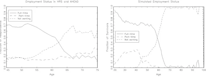
HRS/AHEAD data as a function of age. There is a clear decline in labor force participation starting at about the age of 54. There is also significant increase in part-time work after the age of 60. The simulation results shown on the right hand panel of Figure 1 exhibits a very similar pattern, except that the DP model predicts far less part time work at older ages than is observed in the data. Part of this is an artifact of our classification of part time work in the HRS: we classified individuals who worked between 100 and 1400 hours in a given year as part time workers. Many individuals in this category may be individuals who retired from a full time job part way into a calendar year. It would make more sense to classify such individuals as full time workers: once we adjust for this we expect the observed rates of part-time work will be far less than those shown on the left panel of Figure 1. At the same time we will be adjusting our specification of the DP model to increase the rates of part time work among older individual to better match the (corrected) rates observed in the HRS and AHEAD.

Figure 5 depicts actual and simulated health status. Again, the simulated health status on the right panel of the figure is extremely close to the actual pattern on the left panel of the figure. This is an encouraging result, since health is a vital variable in our model.

Figure 6 provides the results for Social Security status. On the left panel of the figure we present the actual HRS data from the first two waves of the survey, while on the right panel we depict the simulation results. The model captures the main features of the data with reasonable accuracy. The percentage of

7 _{Note we are unable to report the parameter estimates in this proposal since they are based on confidential restricted data on Social} Security earnings records. We are currently seeking approval from the NIH human subjects committee to report these estimates in published articles since there is virtually no way any confidential individual-level information can be inferred from our regression estimates.

population on disability is around 10%. Furthermore, in both panels almost all individuals start receiving OA benefits starting at age 62.

Figure 4: Actual vs. Simulated Labor Force Participation

Figure 5: Actual vs. Simulated Health Status

Figure 7 shows actual and simulated trajectories for wages, and wealth. On the right panel of the figure we also provide the simulated trajectories of Social Security benefits and consumption over the life-cycle. First, we see that wages increased over the first part of the individuals' life-cycle and start dropping in their late 50's in both panels of the figure. During the first 30 years, individuals consumed only about 70% of their wage earnings, resulting in a rapid buildup of net worth that peaks at age 60 in our simulations, and slightly later in the actual data. The maximum level of wealth accumulation is about the same in the data and the simulations, but the life-cycle model predicts a more peaked trajectory for wealth: building up much faster than we observe in the HRS before age 60 and decumulating at a faster rate than we observe after age 60 for older individuals in the HRS and AHEAD. Also the actual distribution of wealth is more skewed than we

observe in the simulations, so that the mean levels of wealth at age 60 is more than twice as high as the median wealth at age 60. The life-cycle model does not result in such a skewed distribution of wealth. We think part of the reason for this discrepancy is that we have ignored income from other sources in the life cycle model, such as spousal income and inheritances. We think that a more realistic version of the model, which would take into account these other sources of income will produce more skewed distributions of wealth as observed in the data. We also believe that account for other risks such as the risk of job loss (involuntary unemployment) and uninsured medical costs, the life-cycle model will predict substantially higher precautionary savings rates than we observe in the current model where the main risks are loss of job due to health problems, mortality, and uncertainty about future wage rates. We also think that more careful treatment of asset illiquidity and transactions costs associated with many durable goods such as housing will also result in larger, more skewed wealth distributions. Also, modeling liquidity constraints and transactions costs associated with housing will probably lead to much slower rates of decumulation of wealth after retirement.8

Figure 6: Actual vs. Simulated Social Security Status

Figure 7: Wealth, Earnings, Social Security Benefits, and Consumption

8 _{Fernández-Villaverde and Krueger (2001), and Bertola, Guiso, and Pistaferri (2001) present models that include durable goods in} life cycle models with uncertainty.

Overall we think the simulation results provide a very good first approximation to the data. Similar to the Engen et al. (1999) simulation findings, we see little evidence that individuals in the HRS cohorts are undersaving for retirement, a conclusion supported by direct empirical analyses of wealth and pension accumulations in the HRS by Gustman and Steinmeier (1999).

The life-cycle model does show how wealth accumulation plays an important role in life-cycle

consumption smoothing. In particular, the rapid decumulation of wealth after retirement allows individuals to maintain a relatively smooth pattern of consumption over their life cycle (with a drop around the age of retirement counterbalanced in utility terms by a substantial increase in leisure), even when major changes in labor supply, and available resources, occur.

Figure 8 compares simulated and actual distributions of age of first entitlement to OA benefits. Again, both the actual and the predicted data have the same main feature: most individuals start receiving benefits at age 62. In the actual data there also a second, much smaller, peak at age 65, which the life-cycle model overpredicts. Notice the clear trend toward early retirement compared with the evidence from the 1970s, analyzed for example in Rust and Phelan (1997). This change has also been mentioned by Gustman and Steinmeier (2002), however, they do not use entitlement rates but a measure of retirement from the labor force, which do not necessarily coincide.

Figure 8: Actual vs. Simulated Distribution of Age of First Entitlement to OA Benefits

Note that there is no heterogeneity in the life-cycle model other than that which is produced by randomly evolving incomes, average wages, and health. We feel that our life cycle model matches the observed distribution of retirement ages quite well given the limited amount of heterogeneity currently in the model. In future work we expect that inclusion of additional sources of observed and unobserved

heterogeneity will enable us to match the observed distribution of retirement ages more precisely. Figure 9 compares the distribution of ages of first entitlement for DI benefits. In this case our

simulations are qualitatively similar to the actual distribution, except that the life-cycle model underpredicts the mean age of first receipt of DI benefits by 3 years. We believe that with additional experimentation on the form of the time and “hassle/stigma” costs associated with applying for DI benefits we will be able to provide a much more accurate approximation to the distribution of ages of eligibility for DI benefits.

Figure 9: Distribution of Age of First Entitlement to DI Benefits

We conclude with Figure 10, which shows two more interesting implications of the life-cycle model. The left panel shows the distributions of bequests. It is highly skewed, with a small number of relatively large bequests. However, none of the bequests in our simulation of 300 relatively lower income individuals exceeded the $600,000 exemption that would have subjected them to Federal estate taxes. Although there is no direct data on the size of bequests in the HRS, there has been some work using the first two waves of the AHEAD by Hurd and Smith (2001), which indicates that our simulations are not unreasonable, and that the distribution of bequests is indeed skewed, but seem to understate the level of bequests. We plan to update part of their work in order to be able to appropriately characterize this aspect of the model. If necessary, we also plan to seek out other sources of data (including probate records) to check the predictions of our model.

Figure 10: Implied Distributions of Bequests and IRRs on Social Security Contributions

The right panel of Figure 10 plots the distribution of internal rates of return (IRR) on Social Security contributions implied by our model. For each of the 300 people in our simulation, we computed the IRR on Social Security contributions---i.e., the interest rate which equates the discounted value of Social Security

taxes (including the employer share) to the present value of Social Security benefits (including disability benefits). We can see that consistent with other studies using actual Social Security benefits, the average internal rate of return on Social Security is quite low---less than 2%. This low internal rate of return is the main cost of continuing to operate a fundamentally pay-as-you-go Social Security system in a rapidly aging society. It is quite easy to re-solve the life-cycle model without any Social Security at all. Individuals lose the valuable risk-sharing features of the current Social Security program but are freed from the restriction of having to make forced contributions to a program that offers very poor rates of return. It is not difficult to compute compensating variations as a function of an individual's current state: this is the amount a person would pay (or need to be paid) as a “bribe” to be released from the current Social Security system. Due to space constraints we do not show these calculations here, but note that our preliminary calculations show just the pattern we would expect: young people (i.e., those younger than age 50) would pay a substantial fraction of their wealth to be released from Social Security. However, old people, having already paid most of their Social Security contributions and who are looking forward to receiving their Social Security benefits would pay an even larger share of their wealth in order to keep the status quo. We can average these person-specific bribes over the population distribution of consumers and determine whether the young in aggregate are willing to pay enough to the old to compensate them for abandoning the system and moving to a fully privatized system. We are not suggesting here that a fully privatized social security is the best possible alternative to the status quo. Our point here is simply to illustrate how the life-cycle model can be used to conduct welfare analyses and analyze the distributional consequences and relative efficiency of alternative proposed policies (assuming lump sum transfers are possible) in a way that is not heavily dependent on subjective interpersonal utility comparisons. We go into further detail about this issue in section 6.

We believe these results show the richness and the insights that can be obtained by taking the effort to formulate and solve a reasonably realistic version of the life-cycle model. We also believe these results show that the model is already empirically promising. If we define an “empirically realistic” model as one that is consistent with the main “stylized facts” of observed behavior, then our model seems at the very least to be the ballpark. We intend to subject our model to much more rigorous tests that can be viewed as the statistical equivalents of the “Turing test”: i.e., will an average researcher be able to distinguish “artificial data” generated from stochastic simulations of our life-cycle model from real data such as we have in the

HRS/AHEAD? We have a lot of work to do before we can think of posing such tests, since we have noted a number of aspects where this simple model appears to be inconsistent with the data. Much of the focus of the first year of our research will be on extending the model in order to relax some of the restrictive predictions of this prototype model.

We bear in mind a result of Rust (1994) that the dynamic programming model is non-parametrically unidentified. That is, if we are free to choose any specification for individual's preferences and beliefs we will always be able to construct a sufficiently complicated life-cycle model that can “rationalize” any observed pattern of behavior. Moreover there will generally be infinitely many distinct combinations of preferences and beliefs that will succeed in rationalizing observed behavior. We are not deterred by this theoretical argument about possible lack of identification for two reasons. First, although it is in principle possible to rationalize any observed set of data using a sufficiently complicated life-cycle model, in practice computational constraints do not afford us the luxury of being able to formulate, solve, and estimate

arbitrarily complicated models. Although our research represents a big step forward, our models will still remain highly simplified and unrealistic in many respects, therefore, subject to standard goodness of fit tests that compare the predictions of the model with in-sample and out of sample data.

Those standard tests often indicate that we have solved misspecified models, this is not too surprising, since the models under consideration are just simplified representations of a very complex reality. We do not view the extended life-cycle model as an exact literal description of an individual's true behavior, but only as

a convenient approximation. The relevant question is whether the life-cycle model provides a parsimonious representation of behavior that results in better predictions than other competing statistical models: we believe that the extended life-cycle framework represents the best current framework for modeling the wide range of behaviors we observe in the data.

Because we are aware of the identification problem, in the process of undertaking our planned extensions of our model we will be concerned about the possibility of “overfitting”, i.e., of selecting particular functional forms that enable us to fit the data well in-sample. The concern is that such

“specification searching” will not result in a model that forecasts well out-of-sample. As we noted in the introduction, we plan to subject our model to perhaps one of the most demanding possible types of out-of-sample predictive tests, namely, using the DP model to predict the response of the subjects receiving the 2 for 1 treatment in the TWWIIA demonstration project. If our models fit well both in-sample and in out-off-sample predictive tests, this is about the most that we can hope for. However, the fact that our models may fit and predict well does not “prove” that people are actually behaving “as if” they had solved the life-cycle problem, but it does give us more confidence that the models can be given more weight in policy forecasting exercises. Ultimately the model that predicts the best and is easiest to use will be the “winner”. By coming forward and submitting this proposal we are betting that the life-cycle model will emerge as the winner --- at least for the foreseeable future.

3.2. Econometric Implementation

We briefly describe how our DP models will be estimated and tested econometrically. We partition an individual's state at time

t

,

s

_t, into observed,

x

_t, unobserved,

ε

_t, components, that is

s

_t

=

(

x

_t

,

ε

_t

)

. The individual observes the full state

s

_t, but the econometrician only observes

x

_t. One must account for unobserved states mainly because a model without unobserved state variables would be statistically

degenerate, i.e., it would predict that certain observed combinations of states and decisions would have zero likelihood of occurring. Assume, for the moment, that all choices are discrete, i.e., the individual chooses a decision

d

_t from a finite set of alternatives

C

_t

(

x

_t

)

. Then, there is a well-developed tractable econometric approach (summarized in Rust 1994) for incorporating unobserved states and estimating the unknown parameters of the DP model. Let the number of components of

ε

_t be the same as the number of choices in the choice set

C

(

x

_t

)

. Then

ε

_t

(

d

)

can be interpreted as a component of utility that depends on the decision

d and other unobserved states of the agent. For reasons of computational tractability, we impose the assumption that

x

_t and

ε

_t are conditionally independent

1 1 1 1

(

t

,

t

| , , )

t t t

(

t

| , ) (

t t t

)

p x

₊

ε

₊

x

ε

d

=

p x

₊

x d q

ε

₊ . (11)

We also assume that

ε

_t