EARLY ONLINE RELEASE
This is a PDF preprint of the manuscript that has been
peer-reviewed and accepted for publication.
This pre-publication manuscript may be downloaded,
distributed, and cited. Since it has not yet been formatted,
copyedited, or proofread, there will be a lot of differences
between this version and the final published version.
The DOI for this manuscript is
DOI:10.2151/jmsj.2015-048
The final manuscript after publication will replace the
preliminary version at the above DOI once it is available.
1
Clouds and the Earth’s Radiant Energy System (CERES) data products for climate
2
research
3 4 5
Seiji Kato1, Norman G. Loeb1, David A. Rutan2, and Fred G. Rose2 6
7
1 Climate Science Branch 8
NASA Langley Research Center 9
10
2 Science System & Applications Inc. 11
12 13
Corresponding author address: 14 15 Seiji Kato 16 Mail Stop 420 17
NASA Langley Research Center 18
Hampton, Virginia 23681-2199 19
e-mail: [email protected]
20
Submitted to Journal of the Meteorological Society of Japan.February 2015 21 22 23 24 25 26
Abstract 27
NASA’s Clouds and the Earth’s Radiant Energy System (CERES) project integrates, 28
CERES, Moderate Resolution Imaging Spectroradiometer (MODIS) and geostationary 29
satellite observations to provide top-of-atmosphere (TOA) irradiances derived from 30
broadband radiance observations by CERES instruments. It also uses snow cover and sea 31
ice extent retrieved from microwave instruments, as well as thermodynamic variables 32
from reanalysis. In addition, these variables are used for surface and atmospheric 33
irradiance computations. The CERES project provides TOA, surface and atmospheric 34
irradiances in various spatial and temporal resolutions. These data sets are for climate 35
research and evaluation of climate models. Long-term observations are needed to 36
understand how the earth system responds to radiative forcing. A simple model is used to 37
estimate the time to detect a trend in TOA reflected shortwave and emitted longwave 38 irradiances. 39 40 41 42 43
1. Introduction
44
The earth receives energy from the sun by radiation and emits the energy to space. Non-45
uniform energy distribution over the globe received from the sun is the driver of 46
dynamics and hydrological cycle that redistribute the energy. Understanding spatial and 47
temporal distributions of radiation or the irradiance is critical to understand how energy 48
flows within the earth system. NASA’s Clouds and the Earth’s Radiant Energy System 49
(CERES, Wielicki et al. 1996) project provides top-of-atmosphere (TOA), surface and in 50
atmosphere irradiances. This paper provides descriptions of CERES data products, 51
irradiance uncertainty, and how algorithms used in the CERES process are improved 52
from those used in earlier projects such as Earth Radiation Budget Experiment (ERBE, 53
Barkstrom et al. 1984). By providing improvements by the CERES project, this paper 54
describes the advance in estimating radiation budget from observations after CERES 55
instruments started measurements in 2000. It also provides complementary information to 56
a review paper by Ohmura (2014) published in this journal. In addition, a simple model is 57
introduced to understand the climate feedback and the time to detect TOA irradiance 58
change. 59
To those who are interested in radiation budget before CERES, excellent reviews 60
of history of earth radiation budget estimates are given by Hunt et al. (1986) for pre 61
satellite era, by House et al. (1986) and by Hartmann et al. (1986) for satellite era before 62
ERBE, and by Kandel and Viollier (2005, 2010) after the ERBE era. An overview of the 63
CERES project is given in Wielicki et al. (1996, 1998). The primary objective of the 64
CERES project is to examine the role of cloud and radiation interaction in the Earth’s 65
climate system (Wielicki et al. 1996) although data products produced by the project have 66
been used for a variety of climate research. 67
Currently, two CERES instruments are operated on Terra, two instruments are on 68
Aqua, and one instrument is on Suomi-NPP. CERES instruments on Terra started 69
measurements in March 2000, and those on Aqua started in July 2002. The CERES 70
instrument on Suomi-NPP started measurement in February 2012. All three satellites are 71
on sun-synchronized orbits. Terra and Aqua’s equator crossing time is, respectively, 72
10:30 and 1:30. CERES instruments can scan along and cross track directions (Fixed 73
Azimuth Plane mode). In addition they can scan with rotating azimuth angle (Rotating 74
Azimuth Plane mode) with unrestricted or restricted the azimuth angle. CERES 75
instruments are currently operated in a cross-track scan Fixed Azimuth Plane mode. In 76
this mode, one instrument observes the entire earth daily. Instrument’s footprint size is 77
approximately 20 km. These CERES instruments provide continuous global radiation 78
data for more than a decade for the first time in satellite radiation budget observation 79
history. 80
In the following, we describe the accuracy of CERES instruments in Section 2, 81
CERES data products and the uncertainty in top-of-atmosphere (TOA) and surface 82
irradiances in Section 3, and the variability of TOA and surface radiation budget in 83
Section 4. In section 5, we discuss the value of long-term radiation budget data in 84
evaluating climate models. A simple analytical model is introduced in Section 6 to help 85
in understanding the climate system that CERES instruments are observing. We estimate 86
the time to detect a trend in the top-of-atmosphere shortwave irradiance using the simple 87
model. 88
89
2. Accuracy and stability of CERES instruments
90
CERES instruments have a shortwave channel, a total channel, and a window channel. 91
The accuracy of shortwave CERES instruments is 1% (1σ or k=1) (Wielicki et al. 1995; 92
Loeb et al. 2009a). The accuracy of the longwave radiance derived from the total channel 93
(i.e. nighttime) is 0.5% (k=1) and that derived from total minus shortwave radiances (i.e 94
daytime) is 1% (Loeb et al. 2009a). The accuracy is improved by a factor of two from 95
ERBE instruments (Wielicki et al. 1995). The estimated stability of the shortwave 96
irradiance derived from observations by a CERES instrument is 0.3 Wm-2 per decade 97
(Loeb et al. 2007a). The better accuracy and stability (repeatability and reproducibility, 98
Taylor and Kuyatt 1994) improves the ability of detecting trends although natural 99
variability greatly affects the trend detection uncertainty and the time to detect a trend 100
(Loeb et al. 2007a; Wielicki et al. 2013). Even for a perfect instrument, there is 101
uncertainty associated with a trend estimate because of natural variability or noise, 102
(Leroy et al. 2008; Wielicki et al. 2013). An additional requirement is that long-term 103
measurements need to be without a gap for passive instruments because they do not carry 104
an absolute calibration system on board (Loeb et al. 2009b; Wielicki et al. 2013). 105
106
3. Top-of-atmosphere (TOA) and surface irradiance data products
107
The CERES science team provides instantaneous (Level 2) top-of-atmosphere and 108
surface irradiances by, respectively, the Single Scanner Footprint (SSF) and Clouds and 109
Radiative Swath (CRS) (Rose et al. 2013) data products for every CERES footprint. 110
Gridded (level-3) data products are provided in various temporal scales, 3-hourly 111
(SYNoptic radiative fluxes and clouds, SYN1deg), daily (SYN1deg), and monthly 112
(SSF1deg and SYN1deg). The CRS and SYN data products also include atmospheric 113
irradiances at three pressure levels, 70 hPa, 200 hPa, and 500 hPa. One more higher level 114
product (Level-3B), the CERES-Energy Balanced and Filled (EBAF) products, provides 115
TOA (Loeb et al 2009a, 2012) and surface (Kato et al. 2013) all-sky and clear-sky 116
irradiances. The EBAF-TOA product uses Argo in-situ ocean heat storage measurements 117
to constrain the TOA net irradiance (Loeb et al. 2009a). The EBAF-surface product uses 118
CALIPSO, CloudSat and AIRS observations to correct bias errors in the cloud and 119
temperature and humidity profiles used in the surface irradiance computations by 120
matching computed TOA irradiances with CERES-derived TOA irradiances provided in 121
EBAF-TOA (Kato et al. 2013). 122
123
3.1. CERES algorithms advanced from ERBE algorithm
124
Angular distribution models, which provide anisotropic factors, are needed to derive 125
irradiance from scanner radiance measurements. The anisotropic factor depends on the 126
scene viewed, such as surface type, cloud fraction, optical thickness, cloud top height, 127
and cloud phase, within the field-of-view, in addition to the viewing geometry of the 128
CERES instrument. ERBE relied solely on shortwave and longwave radiances observed 129
by ERBE scanners to identify the scene type (Wielicki and Green 1989). The CERES 130
project collocates MODIS radiances with a 1 km resolution to identify the scene type 131
(Wielicki et al. 1998). CERES angular distribution models use cloud and surface 132
properties derived from MODIS as well as vertical temperature profiles from reanalysis 133
to convert the radiance to irradiance (Loeb et al. 2005). As a result, CERES algorithms 134
can use more precise scene dependent anisotropic factors (Loeb et al. 2003, 2005; Kato 135
and Loeb 2005, Su et al. 2015) compared to the ERBE algorithm that uses only 12 scene 136
types (Green and Avis 1996). Therefore irradiances are improved, especially for clear-137
sky and regional all-sky irradiances (Loeb et al. 2007b). Other subtle differences between 138
ERBE and CERES algorithms include; 1) CERES adopts a more rigorous unfiltering 139
process and scene dependent unfiltering coefficients (Loeb et al. 2001). The unfiltering 140
process corrects instrument spectral response and converts filtered radiances to unfiltered 141
radiances. As a result of the unfiltering process, the unfiltered shortwave irradiance 142
includes all wavelengths reflected by the earth. Similarly the unfiltered longwave 143
irradiance includes all wavelengths emitted by the earth. 2) The CERES team defines the 144
irradiance reference height as 20 km (Loeb et al. 2002). Because of the spherical 145
geometry of the earth, TOA irradiances depend on the altitude where the irradiance is 146
defined. The 20 km reference altitude is determined by computing the effective radius 147
(radius of the earth plus altitude) of the solid disc that intercepts the equivalent amount of 148
solar energy by the earth. The spectral dependent transmission of the atmosphere needs to 149
be considered to compute solar energy intercepted by the earth. Once the irradiance is 150
defined at 20 km, irradiances included in CERES data products are comparable to those 151
computed with a 1D radiative transfer model. Note that the reference level differs from 152
the height where the radiance is observed. The observation altitude is the satellite altitude 153
so that all absorption and scattering below the altitude is included in observed radiances. 154
3) TOA shortwave irradiances include the irradiance reflected through twilight regions 155
where the solar zenith angle is greater than 90° (Kato and Loeb 2003). As a consequence, 156
the reflected irradiance exceeds the TOA downward solar irradiance over the twilight 157
regions. 158
159
3.2. TOA irradiances and their uncertainty
160
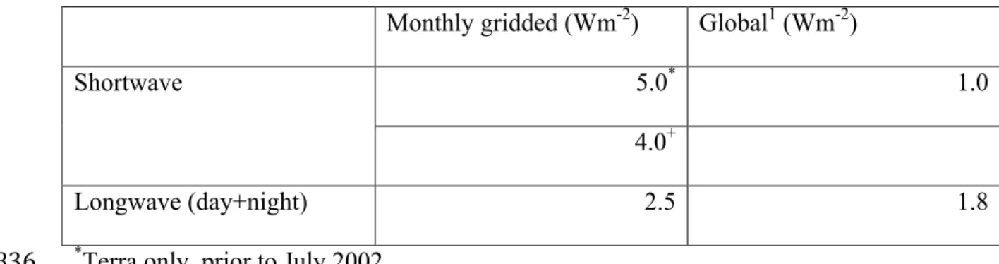
The estimated uncertainty in the monthly 1°×1° latitude-longitude gridded TOA 161
shortwave irradiance is 4 Wm-2 when the irradiance is derived using both Terra and Aqua 162
(i.e. 4 times a day observations for a given location). Prior to July 2002 when only Terra 163
observations are available, the estimated uncertainty in the TOA gridded monthly mean 164
shortwave irradiance is 5 Wm-2. The estimated uncertainty in the TOA gridded monthly 165
mean day plus nighttime longwave irradiance is 2.5 Wm-2 for both Terra only and Terra 166
plus Aqua observations (Doelling et al. 2013). Uncertainties in global monthly and 167
annual mean shortwave and longwave (day+nighttime) irradiance are, respectively, 1.0 168
and 1.8 Wm-2 (Loeb et al. 2009a). Uncertainties in TOA irradiances are summarized in 169
Table 1. 170
As mentioned earlier, the highest level data product is the EBAFTOA and -171
surface products. Because the net TOA irradiance nearly matches ocean heating for a 172
global spatial scale and longer than an annual temporal scale (Loeb et al. 2009a; Loeb et 173
al. 2012), the EBAF-TOA data product uses ocean temperature measurements to adjust 174
TOA-net irradiance to 0.58 Wm-2 (Loeb et al. 2012). To compute the absorbed shortwave 175
irradiance, incoming solar irradiance observed by the Total Irradiance Monitor (TIM) 176
instrument aboard the Solar Radiation and Climate Experiment (SORCE) is used (Loeb et 177
al. 2012). The uncertainty in the net irradiance at a 90% confidence level is ±0.38 Wm-2. 178
For the net irradiance of 0.58 Wm-2, 0.47 Wm-2 is due to heating up to the depth of 1800 179
m, 0.07 Wm-2 is below 2000 m, and 0.04 Wm-2 is due to ice warming and melt (Loeb et 180
al. 2009a). 181
Observing clear-sky radiances by CERES instruments requires cloud free 182
footprints. If only cloud free CERES footprints are taken as clear-sky, the clear-sky 183
irradiance estimate excludes smaller clear-sky area for which the linear dimension is less 184
than about 20 km at nadir. As a result in an extreme case, no monthly mean clear-sky 185
irradiance is provided over a 1°×1° grid where no clear-sky CERES footprints occur over 186
the course of a month. To reduce this sampling problem of TOA clear-sky irradiances, 187
the EBAF product includes clear-sky irradiances derived from MODIS radiances 188
averaged over partly cloudy CERES footprints (Loeb et al. 2009a) in addition to the 189
clear-sky irradiance derived from clear-sky CERES footprints. In addition, the product 190
uses geostationary satellite data to include the diurnal cycle of cloud properties by a 191
similar method described in Doelling et al. (2013). 192
193
3.3. Surface irradiances and their uncertainty
194
The CERES science team also provides surface irradiances in various temporal and 195
spatial scales. We use MODIS derived cloud properties (Minnis et al. 2011), including 196
cloud fraction, cloud top height, optical thickness, particles size, and phase, as inputs for 197
a two-stream radiative transfer model. We also use geostationary satellite-derived cloud 198
properties (fraction, optical thickness, and height) to account for the diurnal cycle of 199
clouds (Rutan et al. 2014). Atmospheric thermodynamic state variables used for 200
computations are from NASA Global Modeling and Assimilation Office (GMAO) 201
reanalysis. Because MODIS-derived aerosol optical thickness is only available for clear-202
sky but the aerosol optical thickness is also needed under cloudy conditions, we use an 203
aerosol transport model (MATCH, Collins et al. 2001) that assimilates MODIS-derived 204
optical thickness. The aerosol transport model also provides aerosol types, which 205
determine the single scattering albedo and asymmetry parameter used in the radiative 206
transfer model. 207
Ocean surface albedo is based on measurements at the Chesapeake lighthouse (Jin 208
et al. 2004). Surface albedos over land are constrained by clear-sky CERES observations 209
(Rutan et al. 2009). The emissivity of land and ocean surfaces is from Wilber et al. 210
(1999). The uncertainty of surface irradiances is given in Table 2. 211
The surface radiation budget and its changes as response to radiative forcing are 212
important for several reasons. First, climate models indicate that the change of 213
precipitation as a response to radiative forcing is driven by surface radiation budget 214
change (Stephens and Ellis 2008). Second, for a global annual scale, the net surface 215
irradiance matches with the sum of surface latent and sensible heat fluxes and ocean 216
heating. Because the latent and sensible heat fluxes are difficult to observe globally, the 217
net surface irradiance might be used to constrain these fluxes. A recent satellite estimate 218
of surface fluxes is given in Stephens et al. (2012). Although, global annual mean net 219
surface irradiance, latent and sensible heat and ocean heating can be forced to balance 220
when all components are altered up to the corresponding 1-sigma uncertainty (L’Ecuyer 221
et al. 2014), a significant discrepancy of approximately 15 Wm-2 exists when all satellite 222
estimates are combined (e.g. Kato et al. 2011). Because the sensible heat is small (23 223
Wm-2, Stephens et al. 2012), the discrepancy is considered to be caused by either the net 224
surface irradiance or latent heat flux, which must balance with precipitation, or both. 225
When CERES EBAF-surface product and Global Precipitation Climatology Project 226
(GPCP, Huffman et al 1997) product are combined with the surface sensible heat flux of 227
17 Wm-2 (Trenberth et al. 2009), the discrepancy is 16 Wm-2 where the net surface 228
irradiance is higher. 229
230
3.4. Evaluation of Surface Irradiance
231
We evaluate computed surface irradiances with observed irradiances at many surface 232
sites. Currently, we use 37 land sites and 49 ocean buoys. Land sites that are used in the 233
evaluation are among the Baseline Surface Radiation Network (BSRN, Ohmura et al. 234
1998) operated by NOAA’s Global Monitoring Division (GMD, Augustine et al. 2000), 235
the US Dept. of Energy’s Atmospheric Radiation Measurement (ARM, Ackerman and 236
Stokes 2003) program, and NOAA’s Global Monitoring Division (GMD) whose data are 237
made available through the NOAA/GMD Solar and Thermal Radiation (STAR) group. In 238
addition, SURFRAD data are made available through NOAA's Air Resources 239
Laboratory/Surface Radiation Research Branch (Rutan et al. 2014). Buoy observations 240
are available from two sources. The Upper Ocean Processes group at Woods Hole 241
Oceanographic Institute has maintained the Stratus, North Tropical Atlantic Site (NTAS) 242
and Hawaii Ocean Time Series (HOTS) buoys. Project Office of NOAA’s Pacific Marine 243
Environmental Labs (PMEL) provides the Tropical Atmosphere Ocean/Triangle Trans-244
Ocean Buoy Network (TAO/TRITON) (McPhaden, 2002), the Prediction and Research 245
Moored Array in the Tropical Atlantic (PIRATA) (Servain et al. 1998), and the Research 246
Moored Array for African - Asian - Australian Monsoon Analysis and Prediction 247
(RAMA) (McPhaden et al., 2009). Detailed descriptions about these validation sites are 248
given in Rutan et al. (2014). 249
When computed monthly 1°×1° gridded mean downward irradiances from EBAF-250
surface Edition 2.8 are compared with 10 years of observed irradiances, the bias averaged 251
over all land and ocean sites are, respectively, -0.9 Wm-2 and 4.0 Wm-2 for surface 252
downward shortwave irradiance and -1.2 Wm-2 and -1.6 Wm-2 for surface downward 253
longwave irradiance (Figure 1). These are well within the estimated uncertainty of daily 254
or annual mean of surface downward of 5 to 6 Wm-2 and downward longwave irradiance 255
of 5 Wm-2 (Ohmura et al. 1998; Colbo and Weller 2009). 256
In addition to the monthly mean irradiance, Figure 2 shows that computed and 257
observed deseasonalized anomalies averaged all sites agree well when time series of 258
irradiance deseasonalized anomalies are compared using data from March 2000 through 259
December 2007 (Rutan et al. 2014). Monthly deseasonalized anomalies are computed by 260
subtracting climatological monthly mean computed for each canonical month using the 261
entire period from the corresponding month. For computed irradiances from EBAF-262
surface Ed. 2.8, 1°×1° grids that contain surface sites are averaged. The correlation 263
coefficient of deseasonalized anomaly time series is 0.95 for both the downward 264
shortwave and longwave irradiances. 265
266
4. Variability of TOA and surface irradiances
267
Researchers recognized that clouds largely influence the albedo of the earth from the 268
beginning of global albedo estimates. Abbot and Fowle (1908a, b) included two types 269
(high and low) of clouds in estimating the global albedo. Regional TOA albedos and 270
cloud radiative effects were estimated by Stephens and Greenwald (1991a, b) from 271
Nimbos-7 Earth radiation budget instruments. Clouds increase the TOA albedo while 272
decreasing outgoing longwave irradiance. One of the ERBE objectives was to investigate 273
which effect is larger and to understand whether clouds warm or cool the planet. A study 274
by Ramanathan et al. (1989) that used April 1985 ERBE data and by Harrison et al. 275
(1990) that used ERBE data from April 1985 through January 1986 concluded that clouds 276
cool the planet, i.e. the cloud radiative effect on TOA albedo is larger than the effect on 277
TOA longwave irradiance. 278
Because cloud radiative effect is defined as the irradiance observed under all-sky 279
condition minus irradiance observed under clear-sly condition, observationally derived 280
cloud radiative effect depends on both cloud properties and clear-sky irradiances (Cess et 281
al. 1987, 1992; Soden 2008, Stevens and Schwartz 2012). Observed mean clear-sky 282
irradiance is weighted by clear-fraction, unlike clear-sky TOA irradiance computed by 283
removing clouds, which samples uniformly. Raschke at al. (2005) and Zhang et al. (1995, 284
2004) use cloud properties from ISCCP (Rossow and Schiffer1991, 1999) and compute 285
TOA irradiances. In their approach, the cloud radiative effect can be computed by 286
removing clouds in the same way that the cloud radiative effect is computed in climate 287
models. CERES also provides computed clear-sky irradiances by removing clouds in 288
SYN1deg and CRS. The difference of the regional shortwave cloud radiative effects by 289
observation and removing clouds is not as large as the difference of longwave cloud 290
radiative effects (Allan and Ringer 2003; Sohn and Bennarts 2008; Sohn et al. 2010; Kato 291
et al. 2013), but large shortwave cloud radiative effect differences occur at high-latitudes 292
(Kato et al. 2013). The difference is caused by clear-sky irradiance difference due to an 293
anti-correlation between sea ice and clouds. Observed clear-sky during sea ice melting 294
season tends to be high because clear-sky tends to occur over sea ice. 295
296
4.1. Albedo variability
297
Because of short lifetime of ERBE scanner instruments and ERBS nonscanners cover 298
only over tropics, only Nimbus-6 and 7 ERB instruments provide observations to analyze 299
interannual variability of global TOA albedo (Smith and Smith 1987; Randel and Vonder 300
Haar, 1990; Smith et al. 1990, Ringer 1997) before observations by CERES instruments 301
on Terra and Aqua. Several studies, however, address the variability of TOA irradiance 302
before CERES. Ringer (1997) used Nimbus-7 data to show that tropical albedo 303
variability is largely caused by ENSO. Wielicki et al. (2002) and Wong et al. (2006) 304
analyzed interannual variability of TOA albedo and emitted longwave irradiance between 305
20°S to 20°N using an ERBE non-scanner on the ERBS satellite. Interannual variability 306
of TOA albedo from 60°N to 60°S derived from Nimbus-7 ERB instruments and its 307
sensitivity to the cloud amount is investigated by Ringer and Shine (1997). 308
Regional cloud amounts over the tropics depend on ENSO (e.g. Klein et al. 1999) 309
and TOA albedo variability over the tropics is highly correlated with cloud amount (Loeb 310
et al. 2007c; Kato 2009). The albedo is also influenced by cloud vertical structure (Cess 311
et al. 2001; Allan et al. 2002; Loeb et al 2012b). 312
313
4.2. Diurnal cycle of albedo
314
Diurnal variability of albedo over the southern Pacific ocean where the diurnal cycle of 315
low-level cloud fraction exists was investigated by Minnis and Harrison (1984). While 316
the cloud amount of marine stratocumulus reaches a maximum in the morning (e.g. 317
Rozendaal et al. 1995), low-level cloud amount over land reaches a maximum in early 318
afternoon (Cairns 1995). Mid and high-clouds reaches maxima in nighttime and early 319
morning (Cairns 1995). The effect of diurnal cycle of cloud properties on albedo was 320
investigated by Hartmann et al. (1991) and Haeffelin et al. (1999). Potter et al. (1988) and 321
Young et al. (1998) discuss the method to include diurnal cycle of albedo in radiation 322
budget estimates from satellite observations. Zhang and Rossow (1995) and Rossow and 323
Zhang (1995) use ISCCP-derived clouds and compute irradiance 3 hourly to include 324
diurnal cycle in radiation budget estimate. The result of Doelling et al. (2013) shows that 325
regional monthly mean reflected TOA shortwave irradiance is influenced by the diurnal 326
cycle of marine stratus and land convective clouds. The global annual mean reflected 327
shortwave irradiance increases by 1% when their diurnal cycle is considered in the 328
estimate (Doelling et al. 2013). However, the effect of the diurnal cycle on the albedo 329
trend and variability over tropics appears to be negligible (Taylor and Loeb 2013). 330
331
5. Using CERES data for climate model validation
332
Mean states form CERES data are used for climate model validations in many studies 333
(e.g. Su et al. 2010; Cheng and Xu, 2011; Cole et al. 2011; Dessler 2013; Xu and Chen 334
2013a, 2013b; Tsushima and Manabe 2013, Painemal et al. 2014). Evaluations by mean 335
states do not necessarily require long-term observations. Long-term radiation budget 336
observations are needed, for example, in evaluating low-level cloud feedback. Prediction 337
of Low-level cloud feedback causes a large uncertainty in predicting climate change. 338
Although recent studies indicate that the cloud feedback is probably a positive feedback 339
(Soden et al. 2008), the cloud feedback parameter estimated from climate models shows a 340
wide spread (Flato et al. 2013; Sherwood et al. 2014). Qu et al. (2014) argue that low-341
level cloud feedback is primarily controlled by two variable changes, the strength of the 342
inversion and sea surface temperature. Most climate models show that the low-level 343
cloud cover increases with inversion strength while it decreases with sea surface 344
temperature (Qu et al. 2014). The ensemble-mean of the estimated inversion strength and 345
sea surface temperature change from CMIP3 and CMIP5 models are both positive. These 346
suggest the sign of the actual cloud feedback depends on the magnitude of the inversion 347
strength, sea surface temperature change and cloud fraction response to them. Most 348
models predict a larger sea surface temperature change than the inversion strength 349
change. Qu et al. (2014) argue that a larger sea surface temperature is physically plausible 350
because surface and 700 hPa air temperature changes are coupled. Their study, however, 351
also reveals that the low-level cloud cover change predicted by climate models depends 352
on parameterization (Qu et a. 2014). Even though cloud parameterization can be 353
evaluated with short term data by comparing, for example, low-level cloud fraction 354
change with sea surface temperature or inversion strength, the cloud feedback is 355
determined by the subtle balance among cloud responses to stability and sea surface 356
temperature, and their change. In addition, other meteorological and cloud property 357
changes might alter the cloud response and stability and sea surface temperature change. 358
These suggest that long-term observations are indispensable in evaluating feedbacks in 359
climate models. 360
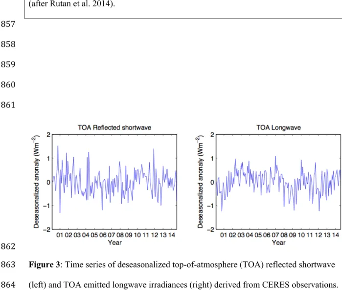
We have nearly 15 years of CERES data (Figure 3). As demonstrated in the next 361
section, fifteen years are too short to determine cloud feedback because of natural 362
variability of TOA irradiances and the signal is too small (Wielicki et al. 2013). Wielicki 363
et al. (2013) estimate that more than 40 years are needed to observe cloud feedback at a 364
95% confidence level with CERES instruments if the cloud radiative effect trend is 5% 365
per decade, which is within a spread of CMIP3 model predictions. 366
It does not mean that, however, efforts to use satellite data to estimate cloud 367
feedback are absent. Dessler (2010, 2013) uses CERES-derived TOA cloud radiative 368
effect with global mean surface temperature to derive cloud feedback parameter, although 369
he recognizes that the feedback parameter derived from a longer record is different from 370
that derived from a shorter time record. In addition, CERES and ISCCP data have been 371
used to estimate TOA irradiance changes responding to sea surface temperature and 372
inversion stability (Eitzen et al. 2011; Qu et al. 2014). In a shorter time scale, dominant 373
causes affecting TOA irradiances are the atmospheric response to ENSO and synoptic 374
systems instead of the response to the radiative forcing due to increasing CO2. TOA 375
irradiance change due to atmospheric response to ENSO or synoptic system is, however, 376
noise to the climate change signal. Then, do we have to wait for multi-decades or even a 377
century of TOA irradiance measurements to evaluate feedbacks in climate models? We 378
argue that the atmospheric response to ENSO or TOA irradiance variability over a shorter 379
time scale provide a useful evaluation for climate models. Because the system generating 380
noise is the same system that responds to the radiative forcing, the variability of TOA 381
shortwave and longwave irradiances contains the information of the response to the 382
radiative forcing although extracting the information is difficult. 383
384
6. Simple analytical model
To demonstrate how the climate change signal appears in the TOA reflected shortwave 386
and emitted longwave irradiances, we constructed a simple model. We also found that 387
such a heuristic 1D ocean and atmosphere model is useful to understand a radiatively 388
forced climate system and the time to detect climate change signals. Note that Hansen et 389
al. (1985) indicate that simple models with an aqua planet tend to underestimate the 390
feedback parameter because ocean heating of an aqua planet is smaller than that of a 391
planet with lands and oceans. In this work, feedback parameters are taken from Table 9.5 392
of IPCC report Chapter 9 (Flato et al. 2013) and the model is used to understand the 393
climate system instead of estimating feedback parameters. 394
The system consists of an ocean effective layer of the depth l of which 395
temperature change ΔT drives the feedback of the system. The feedback parameter is λ-β, 396
where β is the Planck feedback parameter and λ is the sum of all other feedback 397
parameters. We further assume that radiative forcing to the system is a combination of 398
linearly increasing forcing with time with the rate of f and a constant forcing Fa. 399
Radiative forcing increasing with time is due to increasing concentration of carbon 400
dioxide and constant forcing is, for example, due to aerosols. The ocean effective layer 401
transports energy to a deeper layer with a rate h proportional to time (Gregory 2000). The 402
rate of the temperature change of the ocean effective layer is then 403
. (1) 404
To solve Eq. (1), we take a derivative with respect to time, 405 . (2) 406 cpρl dΔT dt =(f −h)t+(λ−β)ΔT+Fa cpρl d2 ΔT dt2 =(f−h)+(λ−β) dΔT dt
The initial condition is ΔT = 0 when t = 0. The solution satisfies both equations and the 407 initial condition is 408 . (3) 409 For β > λ and t>>1, 410 ΔT ≈ Fa λ−β + cpρl(f−h) λ−β
(
)
2 $ % & & ' ( ) )t − Fa f −h+ cpρl β−λ * + , -. / −1 . (4) 411Terms in the square bracket on the right side of Eq. (4) are temperature increase at the 412
time equal to time constants. The first term is the temperature increase needed to offset 413
the aerosol forcing by feedback processes. The second term can be separated into a 414
product of two terms, 415
. (5) 416
The first term on the right side is a time constant and the second term is the rate of the 417
temperature increase. Terms in the parenthesis on the right side of Eq. (4) are also time 418
constants. The first constant Fa
f −his the time when the sum of CO2 forcing and vertical 419
ocean heat transport is equal to the aerosol radiative effect. The second time constant 420
cpρl
β−λ is the time to change the ocean effective layer temperature by 1K by feedback. The 421
second time constant is equivalent to the fast relaxation time scale given by Held et al. 422
(2010) with no vertical energy transport in the ocean. 423 ΔT = Fa λ−β+ cplρ(f −h) (λ−β)2 # $ % & ' ( e λ−β cpρl t − (f −h)t Fa+ cplρ(f −h) λ−β −1 ) * + + + + , -. . . . cpρl(f −h) (λ−β)2 = cpρl β−λ f −h β−λ
The time constant in the parentheses of Eq. (4) that divides time depends on Fa; 424
when Fa<0, the time constant is larger by − Fa
f −hso that it takes longer to reach ΔT than 425
the time when Fa = 0. When the temperature change by Fa is small compared to the 426
second term, the steady state solution is 427
, (6) 428
and the transient climate response is 1/(β-λ) multiplied by the TOA radiative forcing by 429
doubling CO2. 430
We can rewrite Eq. (1) to express the net TOA irradiance. Because the global 431
mean net TOA irradiance agrees with the ocean heating rate for a time scale longer than 432
annual (Loeb et al. 2009a), 433
, (7) 434
where Fsw is the absorbed shortwave irradiance by the system (i.e. the net shortwave 435
irradiance at TOA) and Flw is the upward longwave irradiance at TOA. 436
437
6.1. TOA Shortwave and longwave irradiance trend
438
When radiative forcing and vertical energy transport within the ocean are not time 439
dependent, the TOA net irradiance trend decays with time with the time constant of 440 λ−β cpρl ⎛ ⎝⎜ ⎞ ⎠⎟ −1
. When they are time dependent as expressed in Eq. (7), taking the derivative 441
of Eq. (7) with respect to time, we can compute the trend of the net TOA irradiance. As 442 ΔT ≈ f −h β−λt cpρl dΔT dt +ht= ft+(λ−β)ΔT+Fa =Fsw−Flw
the system approaches a steady state, ΔT linearly increases and the trend of TOA net 443
irradiance decreases approaching . 444
When feedback processes primarily affecting TOA shortwave λsw and longwave 445
λlw irradiances are separated, the net TOA shortwave irradiance change is the rate of 446
temperature change multiplied by the shortwave feedback parameter, 447
. (8) 448
Here, we assume that the radiative forcing does not affect the net TOA shortwave 449
irradiance directly. Similarly, the TOA emitted longwave irradiance change is the sum of 450
the rate of temperature change multiplied by (λlw - β) and the rate of forcing change 451
. (9) 452
Figure 4 shows the trend of the net TOA shortwave irradiance and emitted longwave 453
irradiance. The rate of changing radiative forcing f = 0.049 Wm-2 yr-1 (3.4 Wm-2 divided 454
by 70 years), h = 0.002 Wm-2 yr-1 (0.14 Wm-2 divided by 70 years), Fa = -1.17 Wm-2, and 455
the depth of the ocean effective layer l =150 m are used. The net shortwave trend changes 456
with time and approaches a constant value corresponding to with a time 457
constant of . Similarly, the longwave trend changes with time and approaches a 458
constant value corresponding to with a time constant of . The 459
trend of the net TOA irradiance is f +
(
λ−β)
dΔTdt , which is equal to the trend of ocean
460 f +(λ−β)dΔT dt cpρl d2 ΔT dt2 +h=λsw dΔT dt = λsw cpρl
[
(f −h)t+(λ−β)ΔT+Fa]
cpρl d2ΔT dt2 +h= f +(λlw−β) dΔT dt = f + (λlw−β) cpρl (f −h)t+(λ−β)ΔT+Fa[
]
λsw dΔT dt cpρl λsw f +(λlw−β) dΔT dt cpρl λlw−βheating cpρld 2
ΔT
dt2 +h by Eq. (7). In the following section, a rough estimate of the time 461
to detect the trend of TOA reflected shortwave irradiance is provided. 462
463
6.2. Time to detect a trend
464
The net TOA shortwave and longwave irradiance trends estimated in the previous section 465
can be used to estimate the time to detect trends by a perfect instrument. The effect of 466
instrument calibration uncertainty and sampling uncertainty is discussed in Wielicki et al. 467
(2013). We use the TOA shortwave irradiance trend computed by the simple model as 468
example to estimate the time to detect trend. When the trend of TOA downward 469
shortwave irradiance is negligible, the net shortwave irradiance trend is equal to the 470
reflected shortwave trend and is the shortwave feedback parameter that is due to low-471
level cloud and albedo feedback multiplied by the rate of surface temperature change (Eq. 472
8). We use a formula given by Weatherhead et al. (1998) to estimate of the time to detect 473
the trend of reflected shortwave irradiance because the time series of deseasonalized 474
reflected shortwave irradiances follows a first-order autoregressive model 475
(Phojanamongkolkij et al. 2014). The number of years n* to detect a trend from time 476
series of monthly deseasonalized anomalies is approximated by 477 n* ≈ 2+zβ ω0 σN 1+φ 1−φ # $ % % & ' ( ( 2/3 , (10) 478
where ω0 is the rate of change per year, σN is the standard deviation of deseasonalized 479
anomalies, and φ is the autocorrelation coefficient with lag 1. Using zβ = 0 or 1.3 provides
480
the number of years to detect a trend of magnitude ω0 at the 95% significance level with a 481
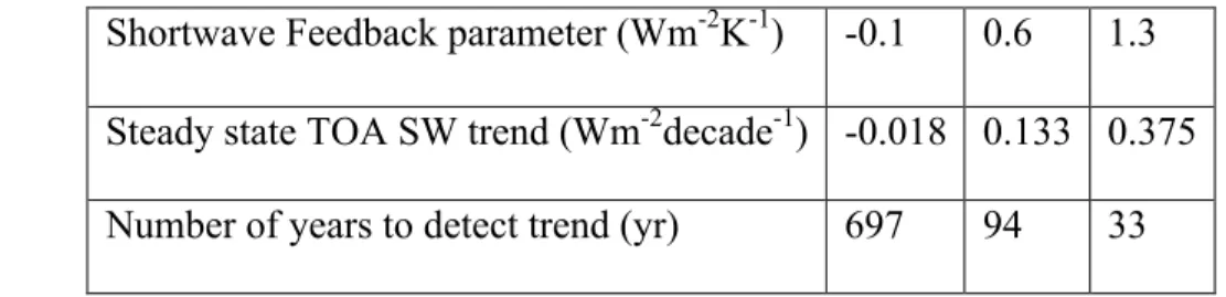
Based on CERES EBAF data, the standard deviation and autocorrelation coefficient of 483
monthly deseasonalized TOA shortwave irradiances are, respectively, 0.545 Wm-2 and 484
0.114. Based on these values and Eq. (25), the number of years to detect a trend of 485
reflected shortwave irradiance with a perfect instrument with a probability of 90% is 486
listed in Table 3. 487
488
7. Summary and conclusions
489
This paper describes TOA and surface irradiance data products produced by the CERES 490
project for climate research. Algorithms used for the process are greatly improved from 491
those used in the ERBE project. The CERES project integrates MODIS and geostationary 492
satellite observations and snow cover and sea ice extent derived from microwave 493
instruments, as well as thermodynamic variables from reanalysis to improve TOA and 494
surface irradiance estimates. It also uses an aerosol transport model that assimilates 495
MODIS-derived aerosol optical thickness. In addition, it uses ocean temperature 496
measurements to constrain the global mean net TOA irradiance for the Level 3B data 497
product. Furthermore, CALIPSO and CloudSat and AIRS observations are used to 498
correct bias error in the cloud, temperature and humidity profiles. The CERES project 499
provides global and regional mean radiation budget at various temporal scales. 500
The length of observations currently available in CERES data products is too 501
short to detect climate feedback and to evaluate feedback processes in climate models. 502
Because the system generating noise is the same system that responds to the radiative 503
forcing, however, the variability of TOA shortwave and longwave irradiances contains 504
the information of the response to the radiative forcing, although the signal may not be 505
easy to extract. The atmospheric response to ENSO or TOA irradiance variability over a 506
shorter time scale, therefore, provides a useful evaluation for climate models. As the 507
observation period extends, radiation budget change might emerge, which can then be 508
used directly to constrain climate models. Earth radation budget observations are 509
therefore indispensable especially when the Earth is changing due to radiative forcing. 510
511 512
References
513
Abbot, C. G., and F. E. Fowle, 1908a: Determination of the intensity of the solar 514
radiation outside the earth’s atmosphere, otherwise termed “the Solar Constant 515
Radiation”, in Annals of the Astrophysical Observatory of the Smithonian 516
Institute, vol2, Chp I, Smithonian Institute, Washington, D. C. 517
Abbot, C. G., and F. E. Fowle, 1908b: Radiatin and terrestrial temperature, in Annals of 518
the Astrophysical Observatory of the Smithonian Institute, vol2, Chp I, 519
Smithonian Institute, Washington, D. C. 520
Ackerman, T. P., and G. M. Stokes, 2003: The atmospheric radiation measurement 521
program, Physics Today, 56, doi:10.1063/1.1554135. 522
Allan, R. P., and M. A. Ringer, 2003: Inconsistencies between satellite estimates of 523
longwave cloud forcing and dynamical fields from reanalyses, Geophys. Res. 524
Lett., 30(9), 1491, doi:10.1029/2003GL017019. 525
Allan, R. P., A. Slingo, and M. A. Ringer, 2002: Influence of dynamics on the changes in 526
tropical cloud radiative forcing during the 1998 El Nino, J. Climate, 15, 1979-527
1986. 528
Augustine, J. A., J. J. DeLuisi, and C. N. Long, 2000: SURFRAD – A national surface 529
radiation budget network for atmospheric research, Bull. Amer. Met. Soc. 81, 530
2341-‐2358. 531
Barkstrom B. R., 1984: The Earth Radiation Budget Experiment (ERBE), Bull. Amer. 532
Meteorol. Soc., 65,, 1170-1185 533
Cairns, B., 1995: Diurnal variation of cloud from ISCCP, Atmospheric Res. 37, 133-146. 534
Cess, R. D. G. L. Potter, W. L. Gates, J.-J. Morcrette, and L. Corsetti, 1992: Comparison 535
of general circulation models to earth radiation budget experiment data: 536
Comparison of clear-sky fluxes, J. Geophys. Res. 97, D18, 20421-20426. 537
Cess, R. D., M. Zhang, P. H. Wang, B. A. Wielicki, 2001: Cloud structure anomalies 538
over the tropical Pacific during the 1997/98 El Nino, Geophy. Res. Lett. 28, 4547-539
4550. 540
Cess, R. D. and G. L. Potter, 1987: Exploratory studies of cloud radiative forcing with a 541
general circulation model, Tellus, 39A, 460-473. 542
Cheng, A., and K.-M. Xu, 2011: Improved low-cloud simulation from a multiscale 543
modeling framework with a third-order turbulence closure in its cloud-resolving 544
model component. J. Geophys. Res., 116, D14101, doi:10.1029/2010JD015362. 545
Colbo, K., and R. A. Weller, 2009; Accuracy of the IMET sensor package in the 546
subtropics, J. Atmos. Oceanic Technol, 26, 1867-1890. 547
Cole, J., H. W. Barker, N. G. Loeb, K. V. Salzen, 2011: Assessing simulated clouds and 548
radiative fluxes using properties of clouds whose tops are exposed to space, J. 549
Climate, 24,2715-2727, DOI: 10.1175/2011JCLI3652.1. 550
Collins, W. D., P. J. Rasch, B. E. Eaton, B. V. Khattatov, J-‐F. Lamarque, and C. S. Zender, 551
2001: Simulating aerosols using a chemical transport model with 552
assimilation of satellite aerosol retrievals: Methodology for INDOEX. J.
553
Geophys. Res., 106 (D7), 7313–7336. 554
Doelling, D. R., N Loeb, D. F. Keyes, M. L. Nordeen, D. Morstad, B. A. Wielicki, D. F. 555
Young, M. Sun, 2013: Geostationary Enhanced Temporal Interpolation for 556
CERES flux products, J. Atmos. Ocean. Tech., DOI: 10.1175/JTECH-D-12-557
00136.1. 558
Dessler, A. E., 2013: Observations of climate feedbacks over 2000-10 and comparisons 559
to climate models, J. Climate, 26, DIO: 10.1175/JCLI-D-11-00640.1. 560
Dessler, A. E., 2013: A determination of the cloud feedback from climate variations over 561
the past decade, Science, 330, 1523, DOI: 10.1126/science.1192546. 562
Eitzen, Z. A., K. M. Xu, T. Wong, 2011: An estimate of low-cloud feedbacks from 563
variations of cloud radiative and physical properties with sea surface temperature 564
on interannual time scales, J. Climate, 24, 1106-1121, doi: 565
10.1175/2010JCLI3670.1. 566
Flato, G., J. Marotzke, B. Abiodun, P. Braconnot, S.C. Chou, W. Collins, P. Cox, F. 567
Driouech, S. Emori, V. Eyring, C. Forest, P. Gleckler, E. Guilyardi, C. Jakob, V. 568
Kattsov, C. Reason and M. Rummukainen, 2013: Evaluation of Climate Models. 569
In: Climate Change 2013: The Physical Science Basis. Contribution of Working 570
Group I to the Fifth Assessment Report of the Intergovernmental Panel on 571
Climate Change [Stocker, T.F., D. Qin, G.-K. Plattner, M. Tignor, S.K. Allen, J. 572
Boschung, A. Nauels, Y. Xia, V. Bex and P.M. Midgley (eds.)]. Cambridge 573
University Press, Cambridge, United Kingdom and New York, NY, USA. 574
Green, R. N., and L. M. Avis, 1996: Validation of ERBS scanner radiances, J. Atmos. 575
Oceanic. Technol. 13, 851-862. 576
Gregory, J. M., 2000: Vertical heat transports in the ocean and their effect on time-577
dependent climate change, Climate Dynamics, 16, 501-515. 578
Haeffelin, M., R. Kandel, and C. Stubenrauch, 1999: Improved diurnal interpolation of 579
reflected broadband shortwave observations using ISCCP data, J. Atmos. 580
Oceanic. Technol. 16, 38-54. 581
Hansen, J., G. Russell, A. Lacis, I. Fung, D. Rind, 1985: Climate response time: 582
Dependence on climate sensitivity and ocean mixing, Science, 229, 857-859. 583
Harrison, E. F. P. Minnis, B. R. Barkstrom, V. Ramanathan, R. D. Cess, G. G. Gibson, 584
1990: Seasonal variation of cloud radiative forcing derived from the Earth 585
Radiation Budget Experiment, J. Geophys. Res., 95, D11, 18687-18730. 586
Hartmann, D., K. J. Kowalewsky, and M. Michelsen, 1991: Diurnal variation of outgoing 587
longwave radiation and albedo from ERBE scanner data, J. Climate, 4, 598-617. 588
Hartmann, D. L., V. Ramanathan, A. Berroir, and G. E. Hunt, 1986: Earth radiation 589
budget data and climate research, Rev. Geophys. 24, 2, 439-468. 590
Held, I. M., M. Winton, K. Takahashi, T. Delworth, F. Zeng, and G. K. Vallis, 2010: 591
Probing the fast and slow components of global warming by returning abruptly to 592
preindustrial forcing, J. Climate, 23, DOI: 10.1175/2009JCLI13466.1. 593
House, F. B., A. Gruber, G. E. Hunt, and A. T. Mecherikunnel, 1986: History of satellite 594
mission and measurements of the Earth radiation budget (1957-1984), Rev. 595
Geophys.., 24, 357-377. 596
Huffman, G. J., and co-authors, 1997: The global precipitation climatology project 597
(GPCP) combined precipitation dataset, Bull. Am. Meteorol. Soc., 78, 5–20. 598
Hunt, G. E., R. Kandel, and A. T. Mecherikunnel, 1986: A history of presatellite 599
investigation of the Earth’s radiation budget, Rev. Geophys. 24, 2, 351-356. 600
Jin, Z., T. P. Charlock, W. L. Smith, Jr., and K. Rutledge, 2004: A parameterization 601
ocean surface albedo. Geophys. Res. Lett., 31, L22301. 602
Kandel, R., M. Viollier, 2010: Observation of the Earth’s radiation budget from space, C. 603
R. Geoscience, 342 286-300, DOI: 10.1016/j.crte.2010.01.005. 604
Kandel, R., M. Viollier, 2005: Planetary radiation budget, Space Science Rev., DOI: 605
10.1007/s11214-005-6482-6. 606
Kato, S., N. G. Loeb, F. G. Rose, D. R. Doelling, D. A. Rutan, T. E. Caldwell, L. Yu, and 607
R. A. Weller, 2013: Surface irradiances consistent with CERES-derived top-of-608
atmosphere shortwave and longwave irradiances, J. Climate, 26, 2719-2740, 609
doi:10.1175/JCLI-D-12-00436.1. 610
Kato, S., N. G. Loeb, D. A. Rutan, F. G. Rose, S. Sun-Mack, W. F. Miller, and Y. Chen, 611
2012; Uncertainty estimate of surface irradiances computed with MODIS-, 612
CALIPSO-, and CloudSat-derived cloud and aerosol properties, Surv. Geophys., 613
Doi 10.1007/s10712-012-9179-x. 614
Kato, S., F. G. Rose, S. Sun-Mack, W. F. Miller, Y. Chen, D. A. Rutan, G. L. Stephens, 615
N. G. Loeb, P. Minnis, B. A. Wielicki, D. M. Winker, T. P. Charlock, P. W. 616
Stackhouse, K.-M. Xu, and W. Collins, 2011, Improvements of top-of-atmosphere 617
and surface irradiance computations with CALIPSO, CloudSat, and MODIS 618
derived cloud and aerosol properties, J. Geophys. Res., 116, D19209, 619
doi:10.1029/2011JD16050. 620
Kato, S., 2009: Interannual variability of global radiation budget, J. Climate, 22, 4893-621
4907, doi: 10.1175/2009JCLI2795.1. 622
Kato, S. and N. G. Loeb, 2005: Top-of-atmosphere shortwave broadband observed 623
radiance and estimated irradiance over polar regions from clouds and the Earth’s 624
Radiant Energy System (CERES) instruments on Terra, J. Geophys. Res. 110, 625
D07202, DOI:10.1029/2004JD005308. 626
Kato, S. and N. G. Loeb, 2003: Twilight irradiance reflected by the Earth estimated from 627
Clouds and the earth’s Radiant Energy System (CERES) measurements, J. 628
Climate, 16, 2646-2650. 629
Klein, S. A., B. J. Soden, N.-C. Lau, 1999: Remote sea surface temperature variation 630
during ENSO: Evidence for a tropical atmospheric bridge, J. Climate, 12, 917-631
932. 632
L’Ecuyer, T., H. K. Beaudoing, M. Rodell, W. Olson, B. Lin, S. Kato, C. A. Clayson, E. 633
Wood, J. Sheffield, R. Adler, G. Huffman, M. Bosilovich, G. Gu, F. Robertson, P. 634
R. Houser, D. Chambers, J. S. Famiglietti, E. Fetzer, W. T. Liu, X. Gao, C. A. 635
Schlosser, E. Clark, D. P. Letternmaier, K. Hilburn, 2015: The observed state of 636
the energy budget in the early 21st century, J. Climate, in press. 637
Leroy, S. S., J. G. Anderson and G. Ohring, 2008: Climate signal detection times and 638
constraints on climate benchmark accuracy requirements. J. Climate, 21, 841-846. 639
Loeb, N. G., J. M. Lyman, G. C. Johnson, R. P. Allan, D. R. Doelling, T. Wong, B. J. 640
Soden, and G. L. Stephens 2012b; Observed changes in top-of-the-atmosphere 641
radiation and upperocean heating consistent within uncertainty, Nature 642
Geosciences, 5, 110-113. doi:10.1038/ngeo1375. 643
Loeb, G. N, B. A. Wielicki, D. R. Doelling, G. L. Smith, D. F. Keyes, S. Kato, N. 644
Manalo-Smith, and T. Wong, 2009a; Toward optimal closure of the Earth’s top-645
of-atmosphere radiation budget, J. Climate, 22, 748-766. 646
Loeb, G. N., B. A. Wielicki, T. Wong, P. A. Parker, 2009b; Impact of data gaps on 647
satellite broadband radiation records, J. Geophys. Res., 114, D11109, 648
doi:10.1029/2008JD011183. 649
Loeb, N. G. and Coauthors, 2007a: Multi-instrument comparison of top-of-atmosphere 650
reflected solar radiation. J. Climate, 20, 575–591. 651
Loeb, N. G., S. Kato, K. Loukachine, M. N. Natividad, and D. R. Doelling, 2007b: 652
Angular distribution models for top-of-atmosphere radiative flux estimation from 653
the Clouds and the Earth’s Radiant Energy System instrument on the Terra 654
Satellite. Part II: Validation, J. of Appl. Meteorol., 24, 564-584. 655
Loeb, N. G., B. A. Wielicki, F. G. Rose, and D. R. Doelling, 2007c: Variability in global 656
top-of-atmosphere shortwave radiation between 2000 and 2005, Geophys. Res. 657
Lett. 34, L03704, DOI:10.1029/2006GL028196. 658
Loeb, N. G., S. Kato, K. Loukachine, and M. N. Natividad, 2005: Angular distribution 659
models for top-of-atmosphere radiative flux estimation from the Clouds and the 660
Earth’s Radiant Energy System instrument on the Terra Satellite. Part I: 661
Methodology, J. of Appl. Meteorol., 22, 338-351. 662
Loeb, N. G., N. Manalo-Smith, S. Kato, W. F. Miller, S. K. Gupta, P. Minnis, and B. A. 663
Wielicki, 2003: Angular distribution models for top-of-atmosphere radiatie flux 664
estimation from the Clouds and the Earth’s Radiant Energy System instrument on 665
the Tropical Rainfall Measureing Mission satellite. Part I: Methodology, J. Appl. 666
Meteorol. 42, 240-265. 667
Loeb, N. G., S. Kato, B. A. Wielicki, 2002: Defining top-of-atmosphere flux reference 668
level for earth radiation budget studies, J. Climate, 15, 3301-3309. 669
Loeb N. G, K. J. Priestly, D. P. Kratz, E. B. Geier, R. N. Green, and B. A. Wielicki, 670
2001: Determination of unfiltered radiances from the Clouds and the Earth’s 671
Radiant Energy System instrument, J. of Appl. Meterol., 40, 822-825. 672
McPhaden, M. J., G. Meyers, K. Ando, Y. Masumoto, V. S. N. Murty, M. Ravichandran, F. 673
Syamsudin, J. Vialard, L. Yu, and W. Yu, 2009: RAMA: The Research Moored 674
Array for African–Asian–Australian Monsoon Analysis and Prediction. Bull.
675
Amer. Meteor. Soc., 90, 459–480. 676
McPhaden, M. J., 2002: TAO/TRITON tracks Pacific Ocean warming in early 2002. 677
CLIVAR Exchanges -‐ eprints.soton.ac.uk, Volume 7, No. 2, pages 7-‐8. 678
Minnis, P. and coauthors, 2011: CERES Edition-2 cloud property retrievals using TRMM 679
VIRS and Terra and Aqua MODIS data, Part I: Algorithms. IEEE Trans. Geosci. 680
Remote Sens. 49, 11, doi: 10.1109/TGRS.2011.2144601. 681
Minnis, P., and E. F. Harrison, 1984: Diurnal variability of regional cloud and clear-sky 682
radiative parameters derived from GOES data. Part III: November 1978 radiative 683
parameters, J. Climate Appl. Meteorol. 23, 1032-1051. 684
Ohmura, 2014: The development and the present status of energy balance climatology, J. 685
Meteor. Soc. Japan, 92, 245-285. 686
Ohmura A., E. Dutton, B. Forgan, C. Frohlich, H. Gilgen, H. Hegne, A., Heimo, G., Konig-‐ 687
Langlo, B. McArthur, G. Muller, R. Philipona, C. Whitlock, K. Dehne, and M. 688
Wild, (1998): Baseline Surface Radiation Network (BSRN/WCRP): New 689
precision radiometry for climate change research. Bull. Amer. Meteor. Soc., 690
79, No. 10, 2115-‐2136. 691
Phojanamongkolkij, N., S. Kato, B. A. Wielicki, P. C. Taylor, M. G. Mlynczak, 2014: A 692
comparison of climate signal trend detection uncertainty analysis methods, J. 693
Climate, DOI: 10.1175/JCLI-D-13-00400.1. 694
Painemal, D., K.-M. Xu, and Anning Cheng, P. Minnis, and R. Palikonda, 2014: Mean 695
Structure and diurnal cycle of Southeast Atlantic boundary layer clouds: Insights 696
from satellite observations and multiscale modeling framework simulations. J. 697
Climate, 28, 324-341. Doi: 10.1175/JCLI-D-14-00368.1 698
Potter, G. L., R. D. Cess, P. Minnis, E. F. Harrison, and V. Ramanathan, 1988: Diurnal 699
variability of the planetary albdo: an appraisal with satellite measurements and 700
general circulation models, J. Climate, 1, 233-239. 701
Qu, X., A. Hall, S. A. Klein, P/ M. Caldwell, 2014: On the spread of changes in marine 702
low cloud cover in climate model simulations of 21st century, Clim. Dyn, 703
42:2603-2626, DOI: 10.1007/s00382-013-1945-z. 704
Ramanathan, V., R. D. Cess, E. F. Harrison, P. Minnis, B. R. Barkstrom, E. Ahmad, D. 705
Hartmann, 1989: Cloud-radiative forcing and climate: Results from the Earth 706
Radiation Budget Experiment, Science, 243, 4487, 57-63. 707
Randel, D. L., and T. H. Vander Haar, 1990: On the interannual variation of the Earth 708
radiation budget, J. Climate, 3, 1168-1173. 709
Raschke, E., A. Ohmura, W. R. Rossow, B. E. Carlson, Y.-C. Zhang, C. Stubenrauch, M. 710
Kottek, and M. Wild, 2005: Cloud effect on the radiation budget based on ISCCP 711
data (1991 to 1995), Int. J. Climatol., 25, 1103-1125. 712
Ringer, M. A., 1997: Interannual variability of the earth’s radiation budget: Some 713
regional studies, Int. J. Climatology, 17, 929-951. 714
Ringer, M. A., and K. P. Shine, 1997: Sensitivity of the Earth’s radiation budget to 715
interannual variations in cloud amount, Climate Dynamics, 13, 213-222. 716
Rose, F. G, D. A. Rutan, T. Charlock, G. L. Smith and S. Kato, 2013: An Algorithm for 717
the Constraining of Radiative Transfer Calculations to CERES-Observed 718
Broadband Top-of-Atmosphere Irradiance. J. Atmos. and Ocean. Tech. 30, 1091-719
1106. DOI: 10.1175/JTECH-D-12-00058.1 720
Rossow, W. B., and R. A. Schiffer, 1999: Advances in understanding clouds from 721
ISCCP, Bull. Amer. Meteor. Soc., 80, 2261-2287. 722
Rossow, W. B., and Y.-C. Zhang, 1995: Calculation of surface and top of atmosphere 723
radiative fluxes from physical quantities based on ISCCP data set 2. Validation 724
and first results, J. Geophys. Res. 100, D1, 1167-1197. 725
Rossow, W. B., and R. A. Schiffer, 1991: ISCCP cloud data products, Bull. Amer. 726
Meteor. Soc., 72, 1-20. 727
Rozendaal, M. A., C. B. Leovy, and S. A. Klein, 1995: An observational study of diurnal 728
cycle variations of marine stratiform cloud, J. Climate, 8, 1795-1809. 729
Rutan, D. A., S. Kato, D. R. Doelling, F. G. Rose, L. T. Nguyen, T. E. Caldwell, and N. 730
G. Loeb, 2014: CERES synoptic product: Methodology and validation of surface 731
radiant flux, Submitted to J. Atmos. Ocean. Tech. 732
Rutan, D., F. Rose, M. Roman, N. Manalo-Smith, C. Schaaf, and T. Charlock, 2009: 733
Development and assessment of broadband surface albedo from Clouds and the 734
Earth’s Radiant Energy System clouds and radiation swath data product. J.
735
Geophys. Res., 114, D08125. doi:10.1029/2008JD010669. 736
Servain, J., A. J. Busalacchi, M. J. McPhaden, A. D. Moura, G. Reverdin, M. Vianna, and 737
S. E. Zebiak, 1998: A Pilot Research Moored Array in the Tropical Atlantic 738
(PIRATA). Bull. Amer. Meteor. Soc., 79, 2019–2031. 739
Sherwood, S. C., S. Bony, and J.-L. Dufresne, 2014: Spread in model climate sensitivity 740
traced to atmospheric convective mixing, Nature, 505, doi:10.1038/nature12829. 741
Smith, E. A., and M. R. Smith, 1987: Interannual variability of the tropical radiation 742
balance and the role of extended cloud system, J. Atmos. Science. 44, 3210-3234. 743
Smith, G. L., D. Rutan, T. P. Charlock, and T. D. Bess, 1990: Annual and interannual 744
variations of absorbed solar radiation based on a 10-year data set, J. Geophys. 745
Res. 95 D10, 16639-16652. 746
Soden, B. J., I. M. Held, R. Colman, K. M. Shell, J. T. Kiehl, and C. A. Shield, 2008: 747
Quantifying climate feedbacks using radiative kernels, J. Climate, 21, 748
doi:10.1175/2007JCLI2110.1. 749
Sohn, B. J., R. Bennartz, 2008: Contribution of water vapor to observational estimates in 750
longwave cloud radiative forcing, J. Geophys Res., 113, doi: 751
10.1029/2008JD010053. 752
Sohn, B. J., T. Nakajima, M. Satoh, and H.-S. Jang, 2010: Impact of different difinitions 753
of clear-sky flux on the determination of longwave cloud radiative forsing: 754
NICAM simulation results, Atmos. Chem. Phys. 10, 11641-11646, 755
doi:105194/acp-10-11641-2010. 756
Stephens, G. L., J. Li, M. Wild, C. A. Clayson, N. Loeb, S. Kato, T. L’Ecuyer, P. W. 757
Stackhouse, M. Lebsock, and T, Andrews, 2012: An update on Earth’s energy 758
balance in light of the latest global observations, Nature Geoscience, 5, DOI: 759
10.1038/NGEO1580. 760
Stephens, G. L. and T. D. Ellis, 2008: Controls of global mean precipitation increases in 761
global warming GCM experiments, J. Climate, 6141-6155. 762
Stephens, G. L., and T. J. Greenwald, 1991a: The Earth’s radiation budget and its relation 763
to atmospheric hydrology 1. Observations of the clear sky greenhouse effect, J. 764
Geophys. Res. 96, D8, 15311-15324. 765
Stephens, G. L., and T. J. Greenwald, 1991b: The Earth’s radiation budget and its relation 766
to atmospheric hydrology 1. Observations of cloud effect, J. Geophys. Res. 96, 767
D8, 15325-15340. 768
Stevens, B., S. E. Schwartz, 2012: Observing and modeling Earth’s energy flows, Surv. 769
Geophys. 33, doi: 10.1007/s10712-012-9184.0. 770
Su, W., J. Corbett, Z. Eitzen, and L. Liang, 2015: Next-generation angular distribution 771
models for top-of-atmosphere radiative flux calculation from the CERES 772
instruments: methodology, Atmos. Meas. Tech. doi: 10.5149/amtd-8-611-2015. 773
Su, W., A. Bodas-Salcedo, K.-M. Xu, and T. Charlock, 2010: Evaluation of the radiative 774
flux and cloud effect profiles in a climate model with the Clouds and the Earth’s 775
Radiant Energy System (CERES) data. J. Geophys. Res., 115, D01105, 776
doi:10.1029/2009JD012490. 777
Taylor, B. N., and C. E. Kuyatt, 1994: Guidelines for evaluating and expressing the 778
uncertainty of NIST measurement results, NIST technical note 1994 edition. 779
Taylor, P. C., N. G. Loeb, 2013: Impact of sun-synchronous diurnal sampling on Tropical 780
TOA flux interannual variability and trend, J. Climate, 26, DOI: 10.1175/JCLI-D-781
12-00416.1. 782
Trenberth, K. E., J. T. Fasullo, and J. Kiehl, 2009: Earth’s global energy budget, Bull. 783
Amer. Meteor. Soc., doi:10.1175/2008BAMS2634.1. 784
Tsushima, Y., and S. Manabe, 2013: Assessment of radiative feedback in climate models 785
using satellite observations of annual flux variation, Proceedings of the National 786
Academy of Sciences 110.19 (2013): 7568-7573. 787
Weatherhead, E. C. and coauthors, 1998: Factors affecting the detection of trends: 788
Statistical considerations and applications to environmental data. J. Geophys. Res., 789
103, 17149-17161. 790
Wielicki, Bruce A., and Coauthors, 2013: Achieving Climate Change Absolute Accuracy 791
in Orbit. Bull. Amer. Meteor. Soc., 94, 1519–1539. 792
Wielicki, B. A., and coauthors, 2002: Evidence for large decadal variability in the 793
tropical mean radiative energy budget, Science, 295, 841-844. 794
Wielicki, B. A. and co-authors, 1998: Clouds and the Earth’s Radiant Energy System 795
(CERES): Algorithm overview, IEEE Trans. Geoscience Remote Sens. 36, 4, 796
1127-1141. 797
Wielicki, B. A., B. R. Barkstrom, E. F. Harrison, R. B. Lee III, G. L. Smith, and J. E. 798
Cooper, 1996: Clouds and the Earth’s Radiant Energy System (CERES): An earth 799
observing system, Bull. Am. Meteorol. Soc., 72, 853–868. 800
Wielicki, B. A., R. D. Cess, M. D. King, D. A. Randall, and E. F. Harrison, 1995: 801
Mission to planet earth: Role of clouds and radiation in climate, Bull. Am. 802
Meteorol. Soc., 71, 2125–2153. 803
Wielicki, B. A. and R. N. Green, 1989: Cloud identification for ERBE radiative flux 804
retrieval. J. of Appl. Meteorol., 28, 11, 1133-1146. 805
Wilber, A. C., D. P. Kratz, and S. K. Gupta, 1999: Surface emissivity maps for use in 806
satellite retrievals of longwave radiation, NASA Tech. Meno., TP-1999-209362, 807
30pp. 808
Wong T., B. A. Wielicki, R. B Lee III, G. L. Smith, K. A. Bush, and J. K. Willis, 2006: 809
Reexamination of the observed decadal variability of the Earth radiation budget 810
using altitude-corrected ERBE/ERBS Nonscanner WFOV Data, J. Climate, 19,
811
4028-4040. 812
Xu, K.-M., and A. Cheng, 2013a: Evaluating low cloud simulation from an upgraded 813
multiscale modeling framework. Part I: Sensitivity to spatial resolution and 814
climatology. J. Climate, 26, 5717-5740. doi:10.1175/JCLI-D-12-00200.1. 815
816
Xu, K.-M., and A. Cheng, 2013b: Evaluating low cloud simulation from an upgraded 817
multiscale modeling framework. Part II: Seasonal variations over the Eastern 818
Pacific, J. Climate, 26, 5741-5760. doi:10.1175/JCLI-D-12-00276.1. 819
Young, D. F., P. Minnis, D. R. Doelling, G. G. Gibson, and T. Wong, 1998: Temporal 820
interpolation methods for the clouds and the Earth’s radiant energy system 821
(CERES) experiment, J. Appl. Meteorol. 37, 572-590. 822