A Solver for the Network Testbed Mapping Problem
Robert Ricci Chris Alfeld∗ Jay LepreauSchool of Computing, University of Utah Salt Lake City, UT 84112, USA {ricci,calfeld,lepreau}@cs.utah.edu
www.flux.utah.edu www.netbed.org
Network experiments of many types, especially em-ulation, require the ability to map virtual resources requested by an experimenter onto available physi-cal resources. These resources include hosts, routers, switches, and the links that connect them. Experi-menter requests, such as nodes with special hardware or software, must be satisfied, and bottleneck links and other scarce resources in the physical topology should be conserved when physical resources are shared. In the face of these constraints, this mapping becomes an NP-hard problem. Yet, in order to prevent map-ping time from becoming a serious hindrance to exper-imentation, this process cannot consume an excessive amount of time.
In this paper, we explore this problem, which we call the network testbed mapping problem. We describe the interesting challenges that characterize it, and explore its application to emulation and other spaces, such as distributed simulation. We present the design, imple-mentation, and evaluation of a solver for this problem, which is in production use on the Netbed shared net-work testbed. Our solver builds on simulated anneal-ing to find very good solutions in a few seconds for our historical workload, and scales gracefully on large well-connected synthetic topologies.
1
Introduction
To conduct a network experiment, the experimenter typically designs the environment in which it will be performed, then instantiates that environment by con-figuring some set of hardware to match it. The primi-tives that describe this environment are nodes and links. For nodes, such as hosts and routers, the experimenter may need specific hardware or software. On links, pa-rameters such as bandwidth and latency are important. For anything larger than a trivial experiment, the pro-cess of selecting and configuring hardware to instanti-ate the desired topology can be tedious and error-prone. The emulation portion of Netbed [22], Emulab, au-tomates this instantiation by taking as input an experi-menter’s topology specification, and configuring it in ∗Now at the University of Wisconsin-Madison, Mathematics
De-partment
real hardware. As part of this automation, Netbed must select appropriate physical resources from those available. This mapping from an experimenter’s vir-tual topology to a physical topology, however, is diffi-cult; it must take into account both the experimenter’s requirements and the physical layout of the testbed. It must give the experimenter appropriate nodes and links, while conserving for other experimenters, scarce physical resources such as bandwidth on network bot-tlenecks. Poor mapping can degrade performance of the emulator or introduce artifacts into an experiment.
We call this problem of selecting hardware on which to instantiate network experiments the network testbed mapping problem. It shares some characteristics with graph partitioning [10] and graph embedding [15], but has domain-specific goals and constraints that make it a different problem and interesting unto itself; these as-pects are the major focus of this paper. We first encoun-tered this mapping problem in our emulation testbed, but it also appears in similar forms in other network experimentation environments.
In formulating and solving this problem, we aim to:
• Make the problem specification broad enough to be applicable to a wide range of network experi-mentation environments;
• Develop abstractions that through their descrip-tion of virtual and physical resources yield power and flexibility; and
• Produce a solver that is able to find near-optimal solutions in a modest amount of time.
In pursuit of these goals, this paper makes the fol-lowing contributions: First, in Sections 2 and 3, it de-fines the network testbed mapping problem, and exam-ines the challenges that make it interesting. Second, in Section 4, it describes our solver for this problem,
assign, which we have been evolving since January
2000, and presents an evaluation of its performance in Section 5. Third, throughout, it presents lessons from our solver’s implementation and its use in Emulab [22], a production network testbed. Fourth, it identifies open issues for future work in Section 7.
2
Environment and Motivation
In order to motivate the network testbed mapping prob-lem, we begin by describing some of the environments to which it is relevant, and identify the characteristics of these environments that make good mapping neces-sary, but difficult.
2.1
Netbed and Emulab
Netbed [22] is a shared public facility for research and education in networking and distributed systems. Ver-sions of it have been in production use since April 2000. One of its goals is to transparently integrate a variety of different experimental environments. Cur-rently, Netbed supports three such environments: em-ulation, simem-ulation, and live-Internet experimentation. Netbed is descended from, and incorporates, Emulab, a time- and space-shared “cluster testbed” whose main goals are to provide artifact-free network emulation for arbitrary experiments, while making that as easy and quick as simulation. Emulab manages a cluster of com-modity PC “nodes” with configurable network inter-connectivity. The facility is space-shared: it can be ar-bitrarily partitioned for use by multiple experimenters simultaneously. Some resources in the system, such as nodes, can only be used in one experiment at a time, although an experiment can be “swapped out” to free resources while it is idle. In that sense, Emulab is also time-shared.
To run an experiment on Emulab, an experimenter submits a network topology. This virtual topology can include links and LANs, with associated characteristics such as bandwidth, latency, and packet loss. Limiting and shaping the traffic on a link, if requested, is done by interposing “delay nodes” between the endpoints of the link. Specifications for hardware and software re-sources can also be included for nodes in the virtual topology.
Once it receives this specification, Emulab must se-lect the hardware that will be used to create the em-ulation. Since Emulab is space-shared, hardware re-sources are constantly changing; only those rere-sources that have not already been allocated are available for use. Currently, the Emulab portion of Netbed tains 168 PCs of varying hardware configurations, con-nected, via four interfaces each, to three switches. In general, large scale emulators require multiple switches, because the number of ports on each switch is limited. Emulab’s switches are connected via inter-switch links; at the present time, these links are 2Gbps. Since multiple experimenters, or even many links from a single experiment, may be sharing these inter-switch links, they become a bottleneck, and overcommitting them could lead to artifacts in experimental results. Be-cause Emulab aims to avoid introducing artifacts due
to its space-shared nature, conservative resource allo-cation is a guiding principle.
In this environment, the mapping algorithm has a number of simultaneous goals. First, it must econ-omize inter-switch bandwidth by minimizing the to-tal bandwidth of virtual links mapped across physical inter-switch links. Second, since not all nodes are iden-tical, the mapping algorithm must take into account the experimenter’s requirements regarding the nodes they are assigned. Furthermore, the mapping must be done in such a way as to maximize the possibility for future mappings; this means not using scarce resources, such as special hardware, that have not been requested by the experimenter. Finally, this mapping must be done quickly. Current experiment creation times in Emulab range from three minutes for a single-node topology, to six and a half minutes for an 80-node topology, though we hope to decrease this time dramatically in the fu-ture. Our goal is to keep the time used by the mapping process much lower than experiment creation time, so that it does not hamper interactive use.
2.2
Simulation: Integrated and Distributed
Netbed integrates simulation with the emulation sys-tem described above. It uses nse [6] to allow the pop-ular ns [5] network simulator to generate and interact with live traffic. This also allows packets generated in the simulator to cross between machines to effect trans-parent distributed simulation. When simulated traffic interacts with real traffic, however, it must keep up with real time. For large simulations, this makes it necessary to distribute the simulation across many nodes. In or-der to do this effectively, the mapping must avoid over-loading any node in the system, and must minimize the links in the simulated topology that cross real physical links.“Pure” distributed simulation also requires similar mapping. In this case, rather than keeping up with real time, the goal is to speed up long-running simu-lations by distributing the computation across multiple machines [4]. However, communication between the machines can become a bottleneck, so a “good” map-ping of simulated nodes onto physical nodes is impor-tant to overall performance. PDNS [17], a parallelized and distributed version of ns, is an example of such a distributed simulator. However, except for certain re-stricted tree topologies, PDNS requires manual parti-tioning onto physical machines.
2.3
ModelNet
Mapping issues also arise in ModelNet [18], a large-scale network emulator which aims at accurate emu-lation of the Internet core through simulating a large number of router queues on a small number of physical
machines. Thus, virtual router queues must be mapped onto physical emulation nodes, known as “core” nodes. In order to minimize artifacts in the emulation, Mod-elNet’s mapping phase, known as “assignment,” must spread queues between the core nodes, to avoid over-loading any one node by giving it a disproportionate share of the traffic. At the same time, it must minimize the bandwidth passing between the core nodes, to avoid overloading their links.
Some aspects of ModelNet mapping are different from those outlined above for Emulab. A major differ-ence is that ModelNet’s is not conservative. To reach its goal of supporting large emulated topologies, Model-Net takes advantage of the fact that not all links will be used to capacity, and allows them to be over-allocated. The goal of ModelNet mapping, then, is minimization of the potential for artifacts, rather than constraint sat-isfaction. Artifacts introduced by over-taxed CPUs or over-used links can be detected by ModelNet, and the emulation topology can be modified to reduce these ar-tifacts in exchange for less accurate emulation of the core.
ModelNet, as currently designed, is not space-shared, meaning that all available resources are used for a single experiment. The goal is to load-balance among these resources, rather than use the least num-ber. ModelNet also has a second phase that includes mapping challenges, called “binding,” in which virtual edges nodes are assigned to physical ones. If the map-ping portions of the ModelNet assignment and binding phases are done in a single pass, as may be necessary in an integrated ModelNet/Emulab environment, there are additional constraints on acceptable solutions intro-duced by IP routing semantics.
We plan to integrate ModelNet into Netbed as an-other emulation mechanism; for this to be seamless, mapping will have to take into account both environ-ments’ goals and resources.
2.4
Similarities
Emulab was the first environment that presented us with the testbed mapping problem. Over several years we developed and improved our solver, targeted exclusively at the Emulab domain. More recently, as we have integrated other network experimentation mechanisms—geographically distributed nodes, simu-lated nodes, and soon ModelNet—to form the general Netbed platform, we immediately faced the mapping issue in each of them.
In the geographically distributed wide-area case, we chose to develop a separate solver [22], based on a ge-netic algorithm; this solver is outlined in Section 7. This was partly due to the degree to which the wide-area problem differed from the Emulab problem, and
partly due to the exigencies of software development. However, the simulated and ModelNet environments are more similar in their mapping needs to Emulab. For example, minimizing inter-switch bandwidth in Emu-lab is similar to minimizing communication between simulator nodes in distributed simulation, and to min-imizing communication between cores in ModelNet. All three environments share a need for mapping that completes quickly. In Emulab and ModelNet, lengthy mapping times discourage experimenters from trying experiments on a variety of configurations, nullifying one of the major strengths of these platforms. In dis-tributed simulation, little benefit is gained from distri-bution of work if the mapping time is a significant frac-tion of the simulafrac-tion runtime.
Therefore, we have extended our solver to handle simulation and ModelNet. The algorithms and pro-gram proved general enough that the extension was not difficult. As reported later in this paper, our initial ex-perience with simulation and ModelNet is promising, although not yet tuned to the degree we have achieved for Emulab. It appears that more environments could be accommodated. Indeed, as outlined in Section 7, with modest work our general solver might handle the wide-area case, should that be desirable.
3
Mapping Challenges
In the context of the environments outlined in the last section, the network testbed mapping problem be-comes the following:
• As input, take a virtual topology and a description of physical resources.
• Map the virtual nodes to physical nodes, ensur-ing that the hardware requirements of the virtual nodes are met.
• Map virtual links to physical links, minimizing the use of bottlenecks in the physical topology.
• In shared environments, maximize the chance of future mappings by avoiding the use of scarce re-sources when possible.
Flexibility in specifying these resources is essential, both for describing available physical resources and re-questing desired virtual topologies.
In this section, we describe the interesting map-ping challenges in more detail. While doing so, we also discuss the abstractions we have designed into our solver, assign, to deal with them, and the ways in which they relate to Emulab and our other target en-vironments. These challenges can be divided into two classes: link mapping and node mapping. We begin by
A Nodes Switches 100Mbit links B C D E F E F D A B C Physical Topology Virtual topology
Figure 1: A trivial six-node mapping problem
describing link mapping, which is applicable across all three target environments. We then address interesting aspects of node mapping, which are of greater specific interest when mapping for Emulab.
3.1
Network Links
One of the key parts of the the network testbed mapping problem is the task of mapping nodes in such a way that a minimal amount of traffic passes through bottleneck links in the physical topology.
The problem can be seen to be NP-hard by reducing the traveling salesman problem to it. Given cities and distances forming an undirected graph G(V, E)with positive integral edge costs, we can create a physical testbed topologyT that corresponds toGby replacing each edge of costc > 1withcedges through chains of switches. We also create a virtual network topology that is a loop of|V|nodes. A solution to the assignment problem will map the virtual loop intoT, minimizing the number of switches. This would then be a solution to the traveling salesman problem. Andersen has also shown the testbed mapping problem to be NP-hard [2], by reducing the multiway separator problem.
Figure 1 shows a trivial example of the mapping problem. The virtual topology on the left is to be mapped onto the physical topology shown to its right. The bandwidths of all virtual and physical links in this example are 100Mbps. To avoid over-burdening the link between the two switches, the sets of nodes
{A,B,C} and{D,E,F} should be assigned to physical nodes that are connected to the same switch. This way, the only virtual link that crosses between switches is the one betweenCandE.
In the virtual topology,assignaccepts two types of network connections: links and LANs. A link is simply a point-to-point connection between two virtual nodes, and includes information such as the bandwidth that it requires. A LAN is specified by creating a vir-tual “LAN node” in the topology, and connecting all members of the LAN to the LAN node using standard links.
At present,assignrecognizes four different types of physical links onto which these virtual links can be mapped. Direct links connect two nodes, without an
intermediary switch. Intra-switch links are those that can be satisfied on a single switch. Inter-switch links must cross between switches. Intra-node links connect nodes run on the same physical node; these links do not need to traverse any network hardware at all, and are used to represent links in distributed simulation or ModelNet that remain on one machine.
When mapping topologies to physical resources, the key limitation is that switch nodes are of finite degree; only a finite number of physical nodes can be attached to a given switch. Neighboring virtual nodes that are attached to the same switch can connect via intra-switch links which traverse only that intra-switch’s back-plane. (This backplane, by design in Emulab, has suf-ficient bandwidth to handle all nodes connected to it, and can thus be considered to have infinite resources.)
To allow topologies that cannot be fulfilled using the nodes of a single switch, Emulab employs several switches, connected together by high-bandwidth links. These inter-switch links, however, do not have suffi-cient bandwidth to carry all traffic that could be put on them by an inefficient mapping. A goal, then, is to minimize the amount of traffic sent across inter-switch links, and use intra-switch links instead, wherever pos-sible. As Emulab is a space-shared facility it is impor-tant that inter-switch traffic be minimized, rather than simply not oversubscribed. By minimizing such traffic, maximum capacity for future experiments is preserved. This problem of minimizing inter-switch connec-tions is similar to sparse cuts in multicommodity flow graph problems—the goal is to separate the graph of the virtual topology into disjoint sets by cutting the minimum number of edges in the graph.
3.2
Node Types
A facility like Emulab will generally have distinct sets of nodes with identical hardware. Emulab, for exam-ple, has 40 600-MHz PCs, and 128 850-MHz PCs. Fa-cilities like this will tend to grow incrementally as de-mand increases, and, to achieve the greatest possible number of nodes, old nodes will continue to be used alongside newly-added hardware. As network testbeds become larger, their hardware will therefore tend to be-come more heterogeneous. With varying node hard-ware, it becomes important for experimenters to be able to request specific types, for example, if they have run experiments on a specific type in the past, and need consistent hardware to ensure consistent results. Of course, experimenters who do not have such require-ments should not be burdened with this specification.
In order to meet this challenge, we have designed a simple type system forassign. Each node in the vir-tual topology is given a type, and each node in the phys-ical topology is given a list of types that it is able to
sat-node sat-node1 pc node node2 pc850 node delay1 delay node delay2 delay
Figure 2: Sample nodes in a virtual topology
node pc1 pc:1 pc850:1 delay:2 node pc2 pc:1 pc850:1 delay:2 node pc3 pc:1 pc600:1 delay:2 node pc4 pc:1 pc600:1 delay:2
Figure 3: Sample nodes in a physical topology
isfy. The fact that a physical node can satisfy more than one type allows for differing levels of detail in specifi-cation, as we will see below. In addition, each type on a physical node is associated with a number indicat-ing how many nodes of that type it can accommodate. This enables multiple virtual nodes to share a physical node, as required for distributed simulation and Mod-elNet. One restriction is invariant, however: all virtual nodes mapped to the same physical node must be of the same type.
To illustrate the type system, consider the fragments of a virtual topology in Figure 2 and a physical topol-ogy in Figure 3. These samples are typical of nodes that are found in Emulab. In this example, virtual
nodenode1can be mapped to any physical node, as
all physical nodes are allowed to satisfy a single pc
node.node2, on the other hand, specifically requests a
pc850, which can only be satisfied bypc1orpc2. In
Emulab, this allows an experimenter to specify a gen-eral class of physical node, such as pc, or request a specific type of PC, such aspc850orpc600.
Virtual nodesdelay1anddelay2can be placed on the same physical node, since all nodes in the phys-ical topology can accommodate two virtual nodes of
type delay. In Emulab, the traffic-shaping nodes,
called delay nodes, that are used to introduce latency, packet loss, etc. into a link, can be multiplexed onto a single physical node; this is possible since delaying a link requires two network interfaces, and four are avail-able on Emulab nodes.
Most types are opaque toassign—there are only two types that are treated specially: switch, which is necessary to support inter-switch links, and lan, which will be discussed in Section 4.2. Thus,assign
is not tied to the hardware types available on Emulab; new types can be added simply by including them in the physical topology.
3.3
Virtual Equivalence Classes
We have found that a common pattern is for experi-menters to care not about which node type they are
allocated, but that all nodes be of the same type. To address this, assignallows the creation of lence classes in the virtual topology. Virtual equiva-lence classes (vclasses) increase the flexibility of the type system, by allowing the user to specify that a set of nodes should be all of the same type, without forcing the user to pick a specific type ahead of time.
vclasses are declarations of virtual equivalence classes in the virtual topology. This includes a list of types that can be used to fulfill thevclass, which could be automatically determined by Emulab. Virtual nodes are then declared to belong to the vclass, rather than a specific physical type. assignwill then attempt to ensure that all nodes in thevclassare assigned to phys-ical nodes of the same type. Multiplevclassescan be used in a virtual topology. This is useful in circum-stances where, for example, the experimenters wants a set of client machines and a set of servers, each of which can be its own class.
vclasses can be of two types, hard or soft. Hard vclasses must be satisfied, or the mapping will fail. Soft vclasses allow assignto break the vclass— that is, use nodes of differing types—if necessary, but homogeneity is still preserved if possible. For soft vclasses, the weight used to determine how much a so-lution is penalized for violating thevclassis included in the virtual topology specification.
3.4
Features and Desires
On a finer granularity than types, assign also sup-ports “features” and “desires.” Features are associated with physical nodes, and indicate special qualities of a node, such as special hardware. Desires are associ-ated with virtual nodes, and are requests for features. Unfulfilled desires—that is, desires of a virtual node that are not satisfied by the corresponding features on the mapped physical node—are penalized in the scor-ing function. Likewise, wasted features—features that exist on a physical node, but were not requested by the virtual node mapped to it—are also penalized.
The chief use of features and desires is to put a pre-mium on scarce hardware. If some nodes have, for ex-ample, extra RAM, extra drive space, or higher-speed links, the penalty against using these features if they are not requested will tend to leave them free for use by experimenters who require them.
Other uses are possible as well. For example, fea-tures and desires can be used to prefer nodes that al-ready have a certain set of software loaded. In Emulab, for example, custom operating systems can be loaded, but features can be used to prefer nodes that already have the correct OS loaded, saving the substantial time it would take to load the OS. Or, if some subset of physical resources have been marked as only usable by
a certain experimenter (for example, by some sort of advance reservation system), those nodes can be pre-ferred.
Specifying features and desires is easy. Since they are represented as arbitrary strings in the input files, like types, they are not restricted to the Emulab en-vironment. Penalties for wasted features can be intu-itively derived. In general, it is sufficient to choose a penalty based on a feature’s relative importance to other resources—for example, one may choose to pe-nalize waste of a gigabit interface more than using an extra link (thus preferring to use another link rather than waste the feature), but less than the cost of us-ing an extra node (thus preferrus-ing to waste a gigabit in-terface before choosing to use another node). Weights can be made infinite, to indicate that a solution failing to satisfy a desire, or wasting a feature, should not be considered a feasible mapping. This is analogous to a hardvclass.
3.5
Partial Solutions
Also useful is the ability to take partial solutions and complete them. These partial solutions can come from the user or from a previous run of the mapping process. In the virtual topology,assigncan be given a fixed mapping of a virtual node onto a physical node, which it is not allowed to change. The two ways in which this feature is used on Emulab are for replacement of nodes in existing topologies and incremental topology changes.
When using a large amount of commodity hardware, failures are not uncommon. When such a failure occurs during a running experiment, the instantiated topol-ogy can be repaired by replacing the failed node or nodes. The topology is run through assign again, with nodes that do not need to be replaced fixed to their existing mapping. This will allow the mapping algo-rithm to select good replacements for the failed nodes. To add or remove nodes from a topology that has al-ready been mapped, a similar strategy is employed. In this case, parts of the topology that have not changed are fixed onto their currently mapped nodes, and new nodes are chosen by the algorithm that fit as well as possible into the existing mapping. In Emulab, this al-lows for the modification of running experiments, sim-ply by supsim-plying a new virtual topology.
4
Design, Implementation, and Lessons
assign, our implementation of a solver for the
testbed mapping problem, is written in 4,800 lines of C++ code. It uses the Boost Graph Library [3] for effi-cient graph data structures, and for generic graph algo-rithms such as Dijkstra’s shortest path algorithm.
Use of a randomized heuristic algorithm helps fulfill the design goals of creating a mapper that is able to find near-optimal solutions in a modest amount of time. For
assign, we have chosen simulated annealing.
Simulated annealing [11] is a randomized heuristic search technique originally developed for use in VLSI design, and commonly used for combinatorial opti-mization problems. It requires a cost function, for de-termining how “good” a particular configuration is, and a generation function, which takes a configuration and perturbs it to create a new configuration. If this new configuration is better than the old one, as judged by the cost function, it is accepted. If worse, it is accepted with some probability, controlled by a “temperature.” This allows the search to get out of local minima in the search space, which would not be possible if only bet-ter solutions were accepted. The algorithm begins by setting the temperature to a high value, so that nearly all configurations are accepted. Over a large number of applications of the generation function (typically, at least in the hundreds of thousands), the temperature is slowly lowered, controlled by a cooling schedule, until a final configuration, the solution, is converged upon. Clearly, this may not be the optimal solution, but the goal of the algorithm is to arrive at a solution near the optimal one.
In this section, we discuss how the functions key to simulated annealing are designed and implemented in
assign. We also introduce two concepts that are key
to the design of assign: violations, which are used to flag whether or not a configuration is acceptable or not, andpclasses, which are equivalence classes used to dramatically reduce the search space.
4.1
Initial Configuration
Typically, simulated annealing is started with a randomly-generated configuration [11]. However, as-signuses a different strategy. assign’s concept of violations, explained later, allows it to begin with an empty configuration—one in which no virtual nodes are assigned to physical nodes. In the generation func-tion, mapping of unassigned nodes gets priority over other transitions. The algorithm must, therefore, spend some time arriving at a valid configuration, but that configuration is likely to be much better than a purely random one, since type information is taken into ac-count.
4.2
Cost Function
assign’s cost function scores a configuration and
re-turn a number that indicates how “good,” in terms of the goals laid out in Section 2, the configuration is. To compute this score, the mappings for all nodes and
links must be considered. Inassign, a lower score is preferable.
Computing the cost for an entire configuration is quite expensive, requiringO(n+l)time, where nis the number of nodes that have been mapped, andl is the number of links between them. If, instead, the cost is computed incrementally, as mappings are added and removed, the time to score a new solution is O(ln), whereln is the number of links connected to the node being re-assigned; this is because, in addition to scor-ing the mappscor-ing of the node itself, all links that it has to other nodes must be scored as well. Clearly, incre-mental scoring provides better scaling to large topolo-gies, so this approach is used inassign. This fits well with simulated annealing, which calls for a generation function that makes small perturbations, which leads naturally to incremental scoring.
assign’s scoring function is split into three parts:
init score initializes the cost for an empty configu-ration, and computes the violations that result from the fact thatassign begins with no nodes mapped. add nodetakes a configuration, a physical nodep, and a virtual nodev. It computes the changes in cost and vi-olations that result from mappingvtop.remove node performs the inverse function, calculating the cost and violations changes that result in unmapping a virtual node.
While incremental scoring greatly reduces the time taken to score large topologies, it does have a cost in the complexity of the scoring function. In particular, care must be taken to ensure that add nodeandremove nodeare completely symmet-ric; remove node must correctly remove the cost added by the correspondingadd node. This is made more difficult by the fact that other mappings may have been added and removed in the time between when a virtual node was mapped and when the mapping is re-moved. In general, though, we feel that the added com-plexity is an acceptable tradeoff for better evaluation times on large virtual topologies.
Link resolution, the mapping of a virtual link to a physical link, is also done in add node—any virtual links associated withvfor which the other end of the link has already been mapped are resolved at this point. This means that links are not first-class objects, subject to annealing. This limits assign’s effectiveness in physical topologies that have multiple paths between nodes, such as nodes that have both direct links to each other and intra-switch links. Our experience, however, is that such topologies do not tend to occur in practice. So, whileassignsupports these topologies, it does not include the additional code and time complexity to treat links as first-class entities. Instead, if multiple link paths are present between a set of nodes,assign
Physical Resource Cost Intra-node Link 0.00 Direct Link 0.01 Intra-switch Link 0.02 Inter-switch Link 0.20 Physical Node 0.20 Switch 0.50 pclass 0.50
Table 1: Scores used inassign
greedily chooses lower-cost links before moving on to higher-cost ones.
To resolve a link, assign finds all possible links between the nodes (direct, intra-switch, and inter-switch) and chooses one. Direct links are used first, if they exist, followed by intra-switch and inter-switch links. To find inter-switch paths, Dijkstra’s shortest path algorithm is run for all switches whenassign
starts. The shortest paths between all switches to which the nodes are connected are then considered possible candidates. If no resolution for a link can be found, a violation is flagged.
A configuration is penalized based on the number of nodes and links it uses. The default penalties, listed in Table 1, can be overridden by passing them toassign
on the command line. Intra-node links, entirely con-tained within a single node and used in mapping sim-ulations, are not penalized at all. Direct node-to-node links, which do not go through a switch, have only a small penalty. Slightly higher is the penalty for intra-switch links. Inter-intra-switch links have a cost an order of magnitude higher, since they consume the main re-source we wish to conserve. A configuration is also penalized on the number of equivalence classes (ex-plained in further detail in Section 4.5) that the chosen physical nodes belong to. This encourages solutions that use homogeneous hardware, which is a quality de-sired by many experimenters. Penalties for unsatisfied desires and unused features are given in the input, and can be chosen based on their relative importance to the resources listed above.
LANs are more computationally costly to score than links, since links involve only two nodes, and their scoring time is thus constant, but LANs can contain many nodes, and their scoring time is linear in the num-ber of nodes that are in the LAN. Inassign, we rep-resent a LAN by connecting its members to a “LAN node,” shown in Figure 4, which is used solely for the purpose of assessing scoring penalties. LAN nodes only exist in the virtual topology—since they do not correspond to a real resource, they are not included in
LAN
A
B
C
D
E
Figure 4: Scoring for LANs is done with a “LAN node,” which LAN members have links to. This LAN uses 3 intra-switch links and 2 inter-switch links.
the input physical topology. As needed, LAN nodes are dynamically bound to switches in the physical topol-ogy, each is attached to the same switch as the major-ity of its members. Thus, any LAN member that is on another switch will be assessed an inter-switch link penalty. Clearly, then, when LAN members are reas-signed, this must be re-calculated, and the LAN node may need to be “migrated” to a new switch, which in-cludes re-scoring all links to it. Doing so is a heavy-weight operation, and the time taken can add more than a factor of three to the runtime for LAN-heavy topolo-gies. Instead, we perform migration only occasionally: when the LAN node is selected for re-mapping by the generation function, and at the end of every tempera-ture step. In practice, we find that this greatly reduces runtime, and has acceptable effects on the solutions found byassign.
4.3
Violations
One issue that must be decided when implementing simulated annealing is whether or not to allow the algo-rithm to consider infeasible solutions; that is, configu-rations that violate fundamental constraints. In the con-text of our problem, the primary constraint considered is over-use of bottleneck bandwidth between switches. The benefits to allowing infeasible solutions, as put for-ward in [1], are twofold. First, this makes the genera-tion funcgenera-tion simpler, as it does not need to take
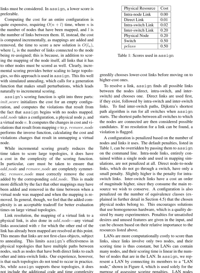
feasi-D B C A D A C B
Figure 5: A situation in which allowing solutions with violations helps reach the optimal solution. If the band-width between switches is such that only one virtual link can cross between them, the mapping shown on the right is in violation of this constraint. However, it is a necessary intermediate step between the mapping on the left and the optimal mapping, which places all nodes on the upper switch.
bility into account. Second, it allows the search to more easily escape local minima, with the possibility that a lower minima will be found elsewhere. It does so by smoothing the cost function. A generation function that excludes infeasible solutions must either simply reject these configurations, or “warp” to a new area of the space, conceptually on the other side of the portion of the space that is infeasible. If infeasible solutions are simply rejected, the connectivity of the solution is re-duced, possibly even leading to portions of the space that are isolated; these could leave the search trapped in a poor local minima. Figure 5 shows an example of this situation. If “warping” is used, the score from a configuration to its potential successor may be very high, resulting in a low probability of its acceptance, even at high temperatures.
A common approach to the search of infeasible con-figurations [1] is to give them a high cost penalty, thus making them possible to traverse at high temperatures, but unlikely to be reached at lower ones. This approach has some drawbacks, however. It is difficult to choose a penalty high enough such that an infeasible solution will never be considered to be better than a feasible one. If this can occur, the algorithm may abandon a fea-sible, but poor, solution and instead return an infeasible one. Thus, inassign, we have chosen to keep track
of the violation of constraints separately from the cost function; this is implemented with “violations.” Each possible configuration has a number of violations as-sociated with it. If a configuration has one or more violations, then it is considered to be infeasible. If no solutions are found with zero violations, the algorithm has failed to find a mapping; frequently, this is because no mapping is possible.
When considering whether or not to accept a state transition, violations are considered before the configu-rations’ costs. If the new configuration results in fewer violations than the old, it is accepted. If the number of violations in the new configuration is equal to or greater than the old violations, then the costs are compared normally. This allows the algorithm to leave feasible space for a time, guiding it back to feasible space fairly quickly so excessive time is not spent on infeasible so-lutions.
One important side effect of violations is that they provide the user of the program with feedback about why a mapping has failed. Six different types of viola-tions are tracked, ranging from overuse of inter-switch bandwidth to user desires that could not be met. These are summed together to produce the overall violations score. Whenassignfails to find a feasible solution, it prints out the individual violations for the best so-lution found. This helps the user to find the “most constraining constraint”; the one whose modification is most likely to allow the mapping to succeed. This gives the user the opportunity to modify and re-submit their virtual topology. It also gives the administrators of the testbed feedback about what factors are prevent-ing experiments from mappprevent-ing, so that they can work on remedying them. It may reveal, for example, that in-sufficient inter-switch bandwidth is a problem, or that experimenters need nodes with more or faster links.
4.4
Generation Function
assign’s generation function has the task of taking a
potential configuration and generating a different, but similar, configuration for consideration.assigndoes this by taking a single virtual node and mapping it to a new physical node. First,assignmaintains a list of virtual nodes that are currently unassigned to phys-ical nodes. If this list is not empty, it picks a member and randomly chooses a mapping for it. If there are no unassigned nodes, it picks a virtual node, removes its current mapping, and attempts to re-map it onto a dif-ferent physical node. If there are no free nodes to which the virtual node can be mapped, it frees one up by un-mapping another virtual node. This is done to avoid getting stuck in certain exact-fit or resource-scarce con-ditions.
We have found that it is very important that
as-sign’s generation function avoid certain classes of in-valid solutions. Though certain violations are useful to explore, as covered in Section 4.3, others are not. In general, violations that cannot be removed by mapping changes to other virtual or physical nodes should be avoided. As an example, a virtual node with five links assigned to a physical node with only four links will always result in a violation, no matter what the rest of the virtual nodes’ mappings are. This is in contrast to an over-used inter-switch link, where changes to other parts of the configuration may lower traffic on the link and remove the violation.
Exploring these invalid solutions can result in poor performance in some cases, particularly when there are scarce resources in the physical topology and only a few nodes in a large virtual topology that require them.
assigncan spend a long time exploring fruitless
por-tions of the solution space in these circumstances. To help avoid certain invalid solutions, when it begins,
assignpre-computes a list of physical nodes that are
acceptable assignments for each virtual node. An ac-ceptable assignment is one that is capable of fulfilling the type of the virtual node, has at least enough physi-cal links to satisfy the virtual node’s links, and will not incur violations due to features and desires.
4.5
Physical Equivalence Classes
4.5.1 Reducing the Solution SpaceOne of the features ofassignthat has most improved its runtime and quality of solutions is the introduc-tion of physical equivalence classes. This improvement comes from the observation that, in a typical network, many hosts are indistinguishable in terms of hardware and network links. For the purposes of the genera-tion funcgenera-tion, these nodes can be considered equiva-lent; mapping a virtual node to any of them will result in the same score. It does not matter which of these in-distinguishable nodes is selected. The solution space to explore can be reduced by exploiting this equivalence.
The neighborhood structure, or branching factor, of a solution space inassignhas a size on the order of O(v·p), wherepis the number of nodes in the physical topology, andvis the set of nodes in the virtual topol-ogy. This number is an upper bound, because, as as-signprogresses, some physical nodes will be already assigned, reducing the number of choices to something less thanp; once all virtual nodes have been assigned, it will beO(v·(p−v)). Clearly, if we can safely re-duce the size ofvorp,assignwill be able to explore a reasonable subset of the solution space in less time, resulting in lower runtimes.
In practice, it is more straightforward, and provides greater benefit, to reducep. The Emulab facility con-sists of a large number of identical nodes connected to
a small number of switches, and other emulation fa-cilities are likely to have similar configurations. For example, in Emulab, depending on available resources, there are 168 PCs that can be in the physical topology input toassign. These reduce to only 4pclasses, resulting in a branching factor two orders of magnitude smaller. Attempting to reducev, on the other hand, will generally not lead to such drastic results, since experi-menters’ topologies are much more heterogenous, and attempting to find symmetries in them would require relatively complicated and computationally expensive graph isomorphism algorithms.
4.5.2 pclasses
In order to effect this reduction in the physical
topol-ogy, assign defines an equivalence relation. Any
equivalence relation on a set will partition that set into disjoint subsets in which all members of a subset are equivalent (satisfy the relation); these subsets are called equivalence classes. When assignbegins it calcu-lates this partition. Each equivalence class is called a pclass.
The equivalence relationassignuses defines two nodes to be equivalent if: they have identical types and features and there exists a bijection from the links of one node to the links of the other which preserves des-tination and bandwidth. It is easily verified that this relation is an equivalence relation.
When the generation function in invoked, rather than choosing a physical node directly, it instead selects a pclass, and a node is chosen from thatpclass. This technique reduces the size of the search space dramat-ically, without adversely affecting quality of solutions found byassign. It reduces the search space by “col-lapsing” areas of the solution space that are equiva-lent. To gain a more intuitive feel for howpclasses reduce the search space, consider two physical nodes with identical hardware and an identical set of links to the same switch. When looking for a physical node to which to map a virtual node, it makes no differ-ence which of these nodesassignchooses, since ei-ther choice will lead to the same score. By combin-ing these two nodes into apclass, and selecting from pclassesrather than nodes, we have combined the two separate states that would result from choosing either of the physical nodes, into a single state. Thus, the branching factor of the search space is reduced, but the set of unique states thatassignvisits is not.
pclasseshave an interesting effect on the way that the solution space is explored; they tend to increase the probability with which physical nodes with scarce resources are selected by the randomized generation function. Selecting from among allpclasseswith the same probability has a higher probability of selecting
a node in a smallpclassthan selecting one in a large pclass. If selecting from among nodes rather than from among pclasses, it is more likely that a node in the largepclasseswill be selected, simply because there are more of them. Thus, we have experimented with weighting the probability that eachpclasswill be se-lected by the number of nodes it contains, to make the probability that each node will be selected similar to what it would be withoutpclasses. However, we have so far found that this is unnecessary, as it does not im-prove the solutions found for our test cases.
There are some circumstances in whichpclassesare not appropriate. When mapping multiple virtual nodes onto each physical node, as is frequently the case with distributed simulations or ModelNet, the base assump-tion, equivalency of certain physical nodes, is violated. As a physical node becomes partially filled, it becomes no longer equivalent to other nodes. Mapping a new virtual node to different physical nodes in the same pclass can now result in different scores, as this af-fects whether some of their virtual links can be sat-isfied as intra-node links or not. As a result, when mapping simulated or ModelNet topologies, we disable pclasses. Fortunately, these mappings tend to involve smaller numbers of physical nodes than full Emulab-style mappings, due to diminishing returns in perfor-mance as the number of physical nodes is increased. Thus, they are still able to complete in reasonable time.
4.6
Cooling Schedule
By default, assign uses the polynomial-time cool-ing schedule described in [1]. It uses a meltcool-ing phase to determine the starting temperature, so that initially, nearly all configurations are accepted. It generates a number of new configurations equal to the branching factor (as defined in Section 4.5) before lowering the temperature. The temperature is decremented using a function that helps ensure that the stationary distribu-tion of the cost funcdistribu-tion between successive tempera-ture steps is similar. Finally, when the derivative of the average-cost function reaches a suitably low value, the algorithm is terminated. The parameters to this cooling schedule were chosen through empirical observation. However, we are exploring the idea of using another randomized heuristic algorithm, such as a genetic algo-rithm, to tune these constants for our typical workload, maximizing solution quality while keeping the runtime at acceptable levels.
The result of this cooling schedule is thatassign’s runtime should scale linearly in two dimensions: the number of virtual nodes, and the number ofpclasses. The temperature decrement function and termination condition, however, will depend on how quickly as-signis able to converge to a good solution, roughly
reflecting the difficulty of mapping the supplied virtual and physical topologies.
assignalso has two time-limited cooling
sched-ules. The first simply takes a time limit, and, using the default cooling schedule, terminates annealing when the time limit is reached. The second mode attempts to run in a target time, even extending the runtime if necessary. It uses a much simpler cooling schedule in which the initial temperature is determined by melting, the final temperature is fixed, and the temperature is decreased multiplicatively, with a constant chosen such that annealing should finish at approximately the cho-sen time. Both of these cooling schemes are useful in limiting the runtime for large topologies, which oth-erwise could take many minutes or even hours to run. The latter is also useful for estimating the best solution to a given problem, as assigncan be made to run much longer than normal, in the hope that it will have a better chance of finding a solution near the optimal one.
5
Evaluation
In this section, we evaluate the performance of as-sign. First, we consider the performance of as-signon a real workload—a set of virtual and phys-ical topology files collected on Emulab over a period of 17 months. Then, we use a synthetic workload to determine howassignwill scale to larger virtual and physical topologies, and to examine the impact of some features and implementation decisions. Then, we ex-amineassign’s ability to map simulated and Mod-elNet topologies. Finally, we compareassignto an-other mapper that we have implemented using a genetic algorithm instead of simulated annealing.
Evaluation is primarily done in two ways: through the runtime ofassign, and through the quality of the solutions it produces. To compare the quality of solu-tions, we compute the average error for each test case. Ideally, the average error is defined as medianopt−opt, whereoptis the optimal score, andmedianis the me-dian of scores across all trials. However, since it is intractable to compute the true value ofopt, we sub-stitutemedianmin−min, whereminis the minimum score found byassignfor the test case. This standard met-ric gives a good feel for the differing scores found by
assignover repeated runs on the same topology.
All tests were performed on a 2.0 GHz Pentium 4 with 512 MB of RAM.
5.1
Topologies from Emulab
Our first set of tests were done using historical data collected from Emulab. The 3,113 test cases are virtual topologies submitted by experimenters, and the
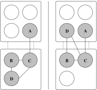
physi-0 0.5 1 1.5 2 2.5 3 0 20 40 60 80 100 Time (s)
Number of Virtual Nodes
Median Time Per Test Case Average of All Test Cases Per Topology Size
Figure 6: Runtimes for Emulab topologies. Each test case was run 10 times. The scatter-plot shows the me-dian runtime for each test case. The line shows the average across all topologies of the same size.
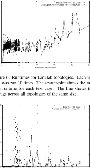
0 0.05 0.1 0.15 0.2 0.25 0 20 40 60 80 100 Error
Number of Virtual Nodes
Error Per Test Case Average Error Per Topology Size
Figure 7: Error for Emulab topologies.
cal topology available at the time the experiment was submitted. Since virtual topologies vary widely, along with available physical resources, the goal of these tests is not to show trends such as scaling to a large num-ber of virtual nodes. Instead, the goal is to show that
assignhandles the typical workload on Emulab very
well.
Figure 6 shows runtimes for the test cases. This graph shows three important things. First, the major-ity of experiments run on Emulab, and thus, the typical workload forassign, consists of experiments smaller than 20 virtual nodes. Second, the relatively flat run-times up to 30 nodes are caused by lower bounds in
assign—to prevent assign from exiting
prema-turely for small topologies, a lower limit is placed on the number of iterationsassignwill run until it deter-mines that it is done. Finally, we can see thatassign
always completes quickly for its historical workload, in less than 2.5 seconds.
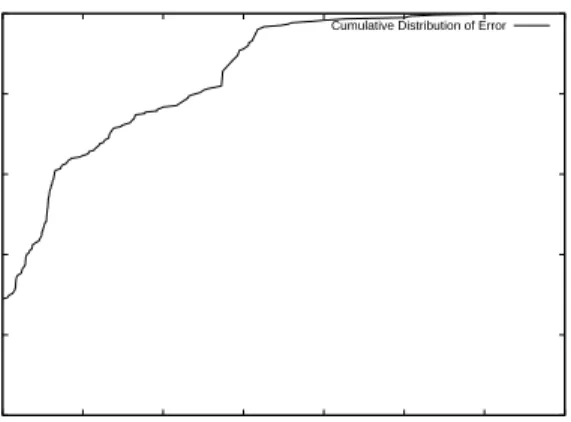
0.9 0.92 0.94 0.96 0.98 1 0 0.05 0.1 0.15 0.2 0.25 0.3 0.35
Fraction of Test Cases at or Below Error
Error
Cumulative Distribution of Error
Figure 8: CDF of error on Emulab topologies. The line represents how many topologies had an error of a given value or smaller. Note that the y-axis for this graph begins at .90.
Figure 7 shows the amount of error for the same test cases, which were each run 10 times. Here, we see that, for virtual topologies of up to 12 nodes,assign
nearly always finds the same solution. Up to 20 nodes, covering most Emulab topologies, the error for most topologies remains below 0.05, or 5%. Even past this range, error stays low. More telling is the Cumula-tive Distribution Function (CDF) for these test cases, shown in Figure 8. Here, we see that approximately 93% of the test cases in this set showed an error of 0, 96% showed an error of less than .05, and over 99% showed an error of less than .17. From this, we can see
that assignis more than adequate for handling the
workload of the present-day Emulab. The tests in later subsections aim to show that assign will scale to larger Emulab-like facilities, in addition to being gen-eral enough for other environments.
5.1.1 Utilization
To evaluate the importance of good mapping to the uti-lization of Emulab’s physical resources, we performed two tests. We used Emulab’s actual physical topology, with the same historical virtual topologies from the last set of tests. In each test, we compared the benefit of us-ing the normalassignwith a version that randomly (instead of near-optimally) obtains a valid mapping of virtual to physical nodes; the random version still ob-serves physical link limits, experimenters’ constraints on node types, etc.
For the first test, we measured throughput. We placed the virtual topologies into a randomly-ordered work queue. Experiments were removed from the queue and mapped, until the mapper failed to find a solution due to overuse of inter-switch bandwidth or lack of free nodes. At that point, the queue stalled
un-til one or more experiments terminated, allowing the experiment at the head of the queue to be mapped. Each experiment was assumed to terminate 24 hours after beginning.Mapping usingassignprocessed the queue in 194 virtual days, while random mapping took 604 days, a factor of 3.1 longer. 1 Limited by trunk
link overuse, random mapping maintained an average of only 5.1 experiments on the testbed. Limited by available nodes,assignmaintained an average of 16 experiments.
For the second test, we used consumption of inter-switch bandwidth as our metric. First, we altered the physical topology to show infinite bandwidth between switches. As above, we first generated a randomly-ordered work queue, then removed and mapped ex-periments until one failed to map by exceeding the number of available nodes. We recorded bandwidth consumption on the inter-switch links. To prepare for the next iteration, we emptied the testbed and re-shuffled the queue. The result, after 30 iterations, was thatassign-based mapping used an average of 0.28Gbps across both links, while random mapping used 7.4Gpbs, a factor of 26 higher.2
To gain further insight intoassign’s value, com-parison against a mapper that uses a simple greedy al-gorithm would also be valuable.
5.2
Synthetic Topologies
For the remainder of our performance results, we use synthetically generated topologies, rather than those gathered from Emulab. One reason for this is that the Emulab topologies vary widely, making it difficult to discern whether trends are due to irregularities in the data, such as topologies with no links, or due to as-signitself. Second, we wish to show thatassign
scales well past the resources currently available on Emulab.
Virtual topologies for these tests were generated us-ing BRITE [14], a tool for generatus-ing realistic inter-AS topologies. A simple Waxman model with random placement was used. This results in topologies that are relatively well-connected, of average degree 4. This provides a good test of assign’s abilities, as such topologies are more difficult to map than ones that have tree-like structures, due to the lack of obvious “skinny” points in the topology.
1The random mapper timed out and could not map 98 large
ex-periments due to overuse of the inter-switch links, even on an empty testbed; we adjusted by assuming they mapped and took the entire testbed.
2The apparent disparity between the ratios in the throughput (3)
and bandwidth consumption tests (26) is explained by observing that for bandwidth, the difference on the bottleneck link between band-width use (5.7Gbps) and capacity (2Gpbs) is what governs job ad-mission in the throughput test; theuse/capacityratio is 2.85.
0 0.5 1 1.5 2 2.5 3 3.5 4 10 20 30 40 50 60 70 80 90 100 Runtime (s)
Number of Virtual Nodes
Maximum Runtime Median Runtime Minimum Runtime
Figure 9: Runtimes for the brite100 test set
0 0.01 0.02 0.03 0.04 0.05 0.06 10 20 30 40 50 60 70 80 90 100 Error
Number of Virtual Nodes
Error
Figure 10: Solution quality for the brite100 test set
The first test set, brite100, consists of 10 topologies ranging from 10 to 100 nodes. The physical topology is similar to Emulab’s, with 120 nodes divided evenly among three switches. The majority of tests are run using this test set, as the randomized nature ofassign
makes it necessary to run a large number of tests to distinguish real overall trends from random effects, and the lower runtimes of this test set make this feasible; each topology in this test case was run 100 times.
The second test set, brite500, is similar to the brite100 test set, but has virtual topologies ranging from 50 to 500 nodes, which are mapped onto a phys-ical topology containing 525 nodes divided evenly across 7 switches.
5.2.1 Scaling
Figure 9 shows runtimes for the brite100 test set. Here, we can see that the mean runtime goes up in an approx-imately linear fashion, and that, for most test cases, the worst-case performance is not much worse than the mean performance. While there is significant variation in the mean runtime, due, we believe, to the relative
0 20 40 60 80 100 120 140 160 50 100 150 200 250 300 350 400 450 500 Runtime (s)
Number of Virtual Nodes
Maximum Runtime Median Runtime Minimum Runtime
Figure 11: Runtimes for the brite500 test set
0 0.01 0.02 0.03 0.04 0.05 0.06 0.07 0.08 0.09 0.1 50 100 150 200 250 300 350 400 450 500 Error
Number of Virtual Nodes
Error
Figure 12: Solution quality for the brite500 test set
difficulty of mapping each topology, the best and worst case runtimes remain very linear.
Figure 10 shows error for the same test set. The low error up to 40 nodes reflects the fact that these topolo-gies can be fit into the nodes on a single switch, and
assignusually finds this optimal solution. For larger,
more difficult, topologies, assign still performs well, with an average of only 5% error.
Figures 11 and 12 show, respectively, the runtimes and error for the brite500 test set. Again, we see linear scaling of runtimes. The slope of the line is somewhat steeper than that of the brite100 set. This is due to the larger physical topology onto which these test cases are mapped.
5.2.2 Physical Equivalence Classes
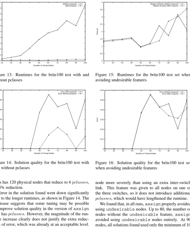
To evaluate the effect thatpclasseshave onassign, we ran it withpclassesdisabled. Runtimes increased by two orders of magnitude, as shown in Figure 13, in which the runtime withpclassesenabled is barely visible at the bottom of the graph. This is primarily due to the fact that the physical topology used for this set of
0 10 20 30 40 50 60 70 80 90 100 10 20 30 40 50 60 70 80 90 100
Average Runtime (seconds)
Number of Virtual Nodes
Without pclasses With pclasses
Figure 13: Runtimes for the brite100 test with and without pclasses 0 0.01 0.02 0.03 0.04 0.05 0.06 10 20 30 40 50 60 70 80 90 100 Error
Number of Virtual Nodes
Error With pclasses Error Without pclasses
Figure 14: Solution quality for the brite100 test with and without pclasses
tests has 120 physical nodes that reduce to 6pclasses, a 95% reduction.
Error in the solution found went down significantly due to the longer runtimes, as shown in Figure 14. The decrease suggests that some tuning may be possible to improve solution quality in the version ofassign
that haspclasses. However, the magnitude of the run-time increase clearly does not justify the extra reduc-tion of error, which was already at an acceptable level. Though error is lower, the minimum-scored solution found both with and withoutpclassesis the same. 5.2.3 Features and Desires
For our first test of features and desires, we examined
assign’s performance in avoiding nodes with
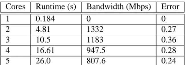
unde-sired features. For this test, we gave 40, or one-third, of the physical nodes in the brite100 physical topology a feature, calledundesirable, which was not desired by any nodes in the virtual topology. We gave this fea-ture a weight that penalizes using anundesirable
0 0.5 1 1.5 2 2.5 3 3.5 4 10 20 30 40 50 60 70 80 90 100 Time (s)
Number of Virtual Nodes
Median Runtime Without Features Median Runtime With Features
Figure 15: Runtimes for the brite100 test set when avoiding undesirable features
0 0.01 0.02 0.03 0.04 0.05 0.06 10 20 30 40 50 60 70 80 90 100 Error
Number of Virtual Nodes
Error Without Features Error With Features
Figure 16: Solution quality for the brite100 test set when avoiding undesirable features
node more severely than using an extra inter-switch link. This feature was given to all nodes on one of the three switches, so it does not introduce additional pclasses, which would have lengthened the runtime.
We found that, in all runs,assignproperly avoided usingundesirablenodes. Up to 80, the number of nodes without the undesirablefeature, assign
avoided using undesirablenodes entirely. At 90 nodes, all solutions found used only the minimum of 10
undesirablenodes, and at 100 nodes, all solutions
used only 20undesirablenodes.
Figure 15 shows runtimes for this test. As we can see, features used in this manner do not adversely affect runtime. Figure 16 compares error for this test case to the cases without features, which is quite similar.
To examine how well assigndoes at finding de-sired features, we again modified the physical topol-ogy from the brite100 set, giving 10% of the nodes feature A, and another 10% feature B. These nodes were spread evenly across all three switches in the
0 1 2 3 4 5 6 7 10 20 30 40 50 60 70 80 90 100 Time (s)
Number of Virtual Nodes
Median Runtime With Features Median Runtime Without Features
Figure 17: Runtimes for the brite100 test set, when at-tempting to satisfy desires
0 0.01 0.02 0.03 0.04 0.05 0.06 10 20 30 40 50 60 70 80 90 100 Error
Number of Virtual Nodes
Error Without Features Error With Features
Figure 18: Solution quality for the brite100 test set, when attempting to satisfy desires
physical topology. This results in a larger number of pclasses(specifically, three times as many) than the base brite100 physical topology, and thus longer run-times. Then, 10% of nodes in the virtual topology were given the desire for featureA, and none given the de-sire for featureB. Thus,assignwill attempt to map certain virtual nodes to the physical nodes with feature
A, and will try to avoid the nodes with featureB. Figures 17 and 18 show the results from this test. As expected, the slope of the runtime line is steeper with these features than without them, due to the fact that they introduce newpclasses. In nearly all tests runs, assign was able to satisfy all desires for featureA. In the 100-node test case, however, failure to satisfy the desire led to a 4% failure rate.
For topologies of size 30 or smaller, which allow a mapping that remains on a single switch without us-ing nodes with featureB, avoiding these nodes is sim-ple, and assignfound such a solution in all of our test runs. For larger topologies, the weight that we
Test Case Nodes selected with featureB
Minimum Median 10 0 0 20 0 0 30 0 0 40 4 4 50 3 4 60 3 4 70 3 4 80 4 4 90 4 4 100 4 4
Table 2:assign’s performance in avoiding featureB
gave to featureB, .5, plays a role in the optimal solu-tion. This weight places the feature as being more valu-able than two inter-switch links, but less valuvalu-able than three. Thus, depending on the virtual topology, it may be desirable forassignto conserve inter-switch links rather than these nodes. Table 2 shows the number of nodes with featureBin the minimally-scored solution, and the median number chosen. If we placed more value on featureB, we could give it a higher weight, so that its cost is higher than a larger number of inter-switch links.
5.3
Distributed Simulation
To test mapping of distributed simulation with as-sign, we first mapped the 500-node topology from the brite500 test set as a simulated topology. To do this, we multiplexed 50 virtual nodes on each of 10 physical nodes. The mapping typically took 46 seconds, with an error of .023.
Second, we applied assign to a large topology generated by the specialized topology generator pro-vided with PDNS. This topology consists of 416 nodes divided into 8 trees of equal height, with the roots of all trees connected in a mesh. In total, this topology contains 436 links. Since the topology generated is of a very restricted nature, the script that generated it is able to optimally partition it to use only 56 links be-tween nodes. Because of its generality,assigndoes not find the same solution. It does, however, typically find a very good solution: the median number of cross-node links found in our test runs was 60. For com-parison, a random mapping of this topology typically results in 385 cross-node links.
The ideal test of the mappings found by assign
for PDNS is to measure the runtime of the distributed simulation, both when mapped byassign, and when using the optimal mapping. However, limitations of
PDNS at the time of writing make it unable to accept arbitrary network partitions, such as those generated by
assign. Newer versions of PDNS, however, may
re-move these limitations and allow us to do this compar-ison.
Running these tests, we encountered unexpected be-havior in assign; it performed very poorly when mapping these topologies as exact-fits. By slightly increasing the number of virtual nodes allowed to be multiplexed on each physical node, we were able to dramatically increaseassign’s solution quality. For example, with the PDNS topology, when each physi-cal node was allowed to host exactly 52 virtual nodes (416/8), the error exceeded 0.4. By allowing each physical node to host 55 virtual nodes, we lowered this error to .05.
It remains an interesting problem for us, then, to analyze this phenomenon and improve assign ac-cordingly. In the case of simulation, it appears we can easily adapt by providing excess “virtual capac-ity.” For physical resources, we would need to im-prove exact-fit matches. Since simulated annealing has fundamental problems dealing with tightly constrained problems [19], this is likely best attacked by improving
assign’s generation function.
5.4
ModelNet
To apply assign to mapping ModelNet, we devel-oped tools to convert ModelNet’s topology represen-tation into assign’s. We then mapped the topol-ogy used in [18] to evaluate ACDC, an application-layer overlay. This topology is a transit-stub network containing 576 nodes to be mapped onto the Mod-elNet core. Transit-transit links have a bandwidth of 155Mbps, transit-stub links have a bandwidth of 45Mbps, and stub-stub links are 100Mbps. The results of mapping this topology to differing numbers of core nodes is shown in Table 3. Though the error is sig-nificantly higher than for the Emulab topologies that
assign has been tuned for, the average bandwidth
to each core node stays near 1000Mbps, which is the speed of the core nodes’ links.
The ModelNet goal of balancing virtual nodes be-tween core nodes can be met in two different ways
withassign. First, the type system can be used to
enforce limits on the number of virtual nodes that can be mapped onto a single ModelNet core. Second, we have implemented experimental load-balancing code in
assignthat attempts to spread virtual nodes evenly
between physical nodes.
Because they use different scoring functions, di-rect comparison between the solutions fromassign
and ModelNet’s mapper is problematic. The best test would be to run both mappers and the resulting
emula-Cores Runtime (s) Bandwidth (Mbps) Error
1 0.184 0 0
2 4.81 1332 0.27
3 10.5 1183 0.36
4 16.61 947.5 0.28
5 26.0 807.6 0.24
Table 3: Performance of assign when mapping a ModelNet topology. The bandwidth shown is the aver-age bandwidth used by each core node to communicate with other cores.
0 50 100 150 200 250 300 350 400 450 500 50 100 150 200 250 300 350 400 450 500 Runtime (s)
Number of Virtual Nodes
Median Runtime - assign Median Runtime - genetic algorithm
Figure 19: Runtimes for the brite500 test set for as-signand our genetic algorithm
tions, and compare the details of their performance and behavior.
5.5
Comparison to Genetic Algorithm
Finally, we compared our simulated annealing ap-proach to the testbed mapping problem to another general-purpose and randomized heuristic approach, a genetic algorithm (GA) [7]. For this test, we indepen-dently implemented another mapper. This mapper uses a standard generational GA, with tournament selection and a specialized crossover operator. The population size is 32, the mutation rate 25%, and the crossover rate 50%. We took care to ensure that the cost func-tions of the two mappers are identical, so that we can compare scores and errors of returned solutions.
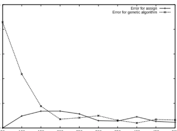
Except for small numbers of nodes, where it was worse, the quality of solutions found by the GA map-per, shown in Figure 20, is close toassign’s. Perfor-mance is a different story. For the brite100 topologies (not shown), the GA was faster when mapping 40 or fewer virtual nodes. However, as shown in Figure 19, the GA exhibited much worse scalability than simu-lated annealing; for all of the brite500 test cases, the GA was slower, on average. At 500 virtual nodes, the
0 0.05 0.1 0.15 0.2 0.25 50 100 150 200 250 300 350 400 450 500 Error
Number of Virtual Nodes
Error for assign Error for genetic algorithm
Figure 20: Solution quality for the brite500 test set for
assignand our genetic algorithm
GA mapper took nearly five times as long asassign. The key reason for this disparity in performance ap-pears to be incremental scoring, which cannot be done in GA’s with crossover. When a new configuration is generated, assignincrementally alters the score. However, the GA relies on a crossover operator that blends two parents to produce two children. Here, incremental scoring is not feasible; childrens’ scores must be entirely re-evaluated. The linearly increasing cost of evaluation is somewhat offset by the GA re-quiring fewer evaluations, on average, than simulated annealing; this accounts for its good performance on small topologies. However, the GA exhibits super-linear scaling as both the cost of evaluations and the number of evaluations required increase.
6
Related Work
Simulated annealing was first proposed for use in VLSI design [11]. Much literature is available on aspects of it [1, 21, 20]. The key problem it was intended to solve was the placement of circuits, which are arranged in a connectivity graph, onto chips. The goal of the map-ping is to minimize inter-chip dependencies, which re-quire communication over expensive pins and busses. In this way, this problem is similar to ours, but does not have the unique challenges described in Section 3. Simulated annealing is also used in combinatorial op-timization in various Operations Research fields.
Similar partitioning problems arise on parallel multi-processor computers [8]. Some network mapping algo-rithms can also be found in the literature. For example, [4] discusses partitioning of distributed simulation us-ing simulated annealus-ing. [12] discusses algorithms for network resources when providing bandwidth guaran-tees for VPNs. None of these, however, meet our goal of being mo