IEEE TRANSACTIONS ON SIGNAL PROCESSING, VOL. 50, NO. 4, APRIL 2002 923
Adaptive Solution for Blind
Identification/Equalization Using Deterministic
Maximum Likelihood
Florence Alberge, Pierre Duhamel, Fellow, IEEE, and Mila Nikolova
Abstract—A deterministic maximum likelihood (DML)
ap-proach is presented for the blind channel estimation problem. It is first proposed in a block version, which consists of iterating two steps, each one solving a least-squares problem either in the channel or in the symbols. In the noiseless case and under certain conditions, this algorithm gives the exact channel and the exact symbol vector with a finite number of samples. It is shown that even if the DML method has a single global minimum, the proposed iterative procedure can converge to spurious local minima. This problem can be detected (under some channel diversity conditions) by using a numerical test that is proposed in the paper.
Based on these considerations, we extend the maximum likeli-hood block algorithm (MLBA) to recursive implementations [max-imum likelihood recursive algorithm (MLRA)]. The MLRA is able to track variations of the system by the introduction of an exponen-tial forgetting factor in the DML criterion. The link between the adaptive algorithm and a soft decision feedback equalizer (SDFE) is emphasized. Low-complexity versions of the recursive and adap-tive algorithm are presented.
Index Terms—Adaptive algorithm, blind equalization,
deter-ministic maximum likelihood method, joint estimation.
I. INTRODUCTION
B
LIND identification/equalization is an important problem in wireless communications, either in a passive listening situation or in fast fading environments. Blind techniques present some advantages compared with the traditional training methods. First, the reduced need for overhead information increases the bandwidth efficiency. Furthermore, in certain communication systems, the synchronization between the receiver and the transmitter is not possible, and thus, training sequences are not exploitable. However, when some symbols are known, “semi-blind” techniques are preferred since they are able to track system variations much more efficiently than algorithms based only on training sequences while having performance much enhanced compared with fully blind al-gorithms. When the known symbols are grouped, maximum likelihood (ML) permits us to obtain easily a semi-blind criterion [1]. Therefore, we choose to focus on blind criteria.Manuscript received June 1, 2000; revised September 13, 2001. The associate editor coordinating the review of this paper and approving it for publication was Prof. Michail K. Tsatsanis.
F. Alberge and P. Duhamel are with the Supelec/LSS, Gif-Sur-Yvette, France (e-mail: [email protected]; [email protected]).
M. Nikolova is with the ENST/TSI and CNRS URA 820, Paris, France (e-mail: [email protected]).
Publisher Item Identifier S 1053-587X(02)02392-9.
The earlier approaches to blind equalization were based on higher order statistics of the received signal [2]–[5]. Although these algorithms are robust and reliable in many cases, esti-mating high-order statistics usually requires a large number of data samples. Hence, their application in a fast varying environ-ment is intrinsically limited. Tong et al. suggested a different option [6]. They make use of time or spatial diversity at the output of the channel, which is obtained when the measured samples are oversampled or when several antennas are used. Thus, the considered system is a single input/multiple output system (SIMO). The SIMO equalization problem can be solved using second-order statistics only, as long as the subchannels do not share common zeros. Second-order techniques have the po-tential for estimating the required statistics with fewer samples; hence, they do not have the intrinsic limitations of higher order ones. However, whether a given method converges faster than another one relies on other properties.
Some second-order methods rely on assumptions on the sta-tistics of the input sequence (usually, an assumption of the se-quence to be white) [7]–[10]. In a fast fading environment, if only a few data samples corresponding to the same channel char-acteristics are available, then the statistical estimate is not reli-able. In that case, the problem may be solved by treating the input as a deterministic variable. This paper focuses on this sit-uation: The input sequence is considered as a deterministic pa-rameter to be identified. More precisely, this paper deals with deterministic maximum likelihood (DML) methods. The good property of DML methods in a SIMO context relies on the fact that it can be obtained through a sequence of least-squares prob-lems, as we will see. However, their main drawback lies in the difficulty to express the estimator in closed form and in the pres-ence of local minima. This is partially solved here in the context of DML.
Among the major contributions to DML methods, we can cite the work of Hua, who proposed in [11] the two-step maximum likelihood (TSML) method. The TSML method establishes a connection between the cross relation (CR) method, which belongs to subspace methods, and the ML estimator. Around the same time, Slock developed a method denoted the iterative quadratic maximum likelihood (IQML) method [12], [13], which is similar to the TSML method. Both methods iterate two steps to estimate the channel. The performance comparison with the Cramér-Rao bound has been obtained in [11], [14], and [15]. Others DML methods are available in [16] and the references therein. DML algorithms are capable of obtaining perfect channel estimation within a finite number of samples 1053–587X/02$17.00 © 2002 IEEE
in the absence of noise. On the other hand, TSML and IQML give biased channel estimates [17] and may behave poorly at low SNR, even with an asymptotical number of data. Ayadi proposed, in [18], two solutions to remedy this situation, which lead to “denoised” ML algorithms. Unfortunately, these deter-ministic algorithms have been developed for batch processing, and their adaptive implementations are often cumbersome. The approach proposed in this paper has the attractive properties of DML with, at the same time, a structure suitable for recursive and adaptive implementation.
This paper is built on a previous work performed in the same team [19], where a block algorithm (MLBA) was proposed. Each step of the MLBA solves a least-squares problem alter-nately in the channel and in the symbols, whereas in previous contributions, either the symbols or the channels were not com-puted explicitly during the iterations. Alternating methods have also been proposed in contributions like [20] or [21], where the finite alphabet property is used. In the absence of noise, the MLBA estimates the channels and symbols perfectly, using a fi-nite number of symbols, and the MLBA has a single global min-imum [19]. Some recursive versions were proposed, including decision devices. The behavior of the algorithm was proved to be very similar to a DFE. Pité wrongly stated in [22] that the MLBA does not admit local minima in the noiseless case. Un-fortunately, the implementation of the MLBA is complicated by the existence of local minima even with noiseless data. The nov-elty of this paper is twofold.
• A numerical test is proposed to circumvent the local minima problem. Actually, we combine the iterative al-gorithm with a growing window technique, and we show that under the classical assumptions of channel diversity and sufficient excitation of the symbols, we are able to check whether the obtained stationary point is the global minimum or a spurious local minimum. This property can be extended to noisy data when a large amount of data is considered.
• A recursive version of the MLBA that does not involve any hard decision is presented. Then, the error propaga-tion problem frequently encountered with the DFE-like al-gorithm (and, thus, with the alal-gorithm proposed by Ges-bert [19]) is solved. Moreover, we prove, in the noiseless case, that when the recursive algorithm converges, then it converges toward the global minimum. System adaptivity is then obtained by introducing an exponential weighting factor in the criterion. The connection between this algo-rithm and the structure of the DFE is emphasized. The re-sulting algorithm is very similar to a DFE where the hard decision is replaced by a soft estimate of all symbols in-volved in the computation of a given channel output. Up-date strategies of the filters can be either of a least-squares type (RLS like) or of a stochastic gradient type (LMS like). Both of them are derived in this paper.
This paper is organized as follows. The general setup and the DML criterion, which is a quadratic minimization problem in both the channels and the symbols, are presented in Section II. For noise-free data, we recall that the global minimum of the DML criterion is unique. Then, in Section III, we derive the
two-steps block iterative algorithm and show that it can con-verge to local minima. A recursive version is derived in Sec-tion IV. We prove that the recursive algorithm converges only toward the global minimum. A simplified version of the recur-sive algorithm is presented in Section IV-D. In Section V-A, we introduce a weighting factor into the criterion, and we ob-tain the adaptive algorithm. A comparison between the struc-ture of our adaptive algorithm and of a DFE is proposed in Sec-tion V-B. The performance of the algorithms and comparison with existing approaches are provided in Section VI.
II. PROBLEMFORMULATION
Let be the continuous-time baseband signal received at the output of a noisy channel
(1)
where denotes the baseband equivalent channel, in-cluding the effects of the emission and reception filters, of the channel response, and of the modulation and demodulation. The symbol sequence is emitted with rate , and stands for some additive independent white Gaussian noise. Consider a fractionally spaced equalizer, the received continuous time
signal being sampled at rate . For , set
and . The discrete time version of
the signal model in (1) may be expressed as
where and are complex variables. This
single-input/multiple-output (SIMO) model can also be used for systems involving multiple receivers. For convenience, we adopt the following notations throughout the paper.
• are variables denoting any channel and any symbol sequence, respectively.
• are the true channels and symbols, respectively, and is the corresponding (noisy) observation.
• are the estimates of and .
• and
is the time index. •
is a vector of length containing symbols estimated at iteration .
The channel impulse responses
are assumed to have a finite length, and stands for the maximum order of any channel. Let
denote the vector obtained by interlacing the outputs of the different channels,
the vector containing transmitted symbols, and . Then, the output reads:
Here, stands for the noise vector. The noise sequences are assumed to be i.i.d., Gaussian, and mutually uncorrelated. In (2), operator transforms a sequence of channel
into the following generalized Sylvester matrix [23]:
. .. . .. . .. ... ..
. . .. . .. . ..
Let be the operator that transforms a vector into a matrix , in such a way that
(3) It can be shown that this matrix reads
.. .
where is the Kronecker product, is the identity
matrix, and . The
results displayed in the paper rely on the following assumptions. H1) has full column rank.
H2) The symbol sequence has linear complexity or greater [24]. The linear complexity of
the sequence is defined as the
smallest value of for which there exists such as
The linear complexity measures the predictability of a finite length deterministic sequence.
H2’) When H2) is met, it can be shown that is full column rank.
H3) (maximum order of the channels) is known or cor-rectly estimated.
Assumption H1) means that there is channel diversity that guarantees that (2) is an overdetermined system of equations for fixed. Similarly, H2’) ensures that (2) is an overdetermined system for fixed. Denote by the matrix
..
. ... ... ...
Then, H2) implies rank .
Hence, the sample covariance of the vector sequence is full rank, and it is seen that the linear complexity property is strongly connected with the notion of persistent excitation [25] of a sequence. We can remark that rank
implies that, necessarily, .
We consider the problem of identifying both and from without using any prior about the transmitted sequence or the channel. Following [11], [13], and [19], are esti-mated through the minimization of the DML criterion with re-spect to the joint variable :
where the second formulation comes from (3). Hence, the esti-mated channels and symbols read
(4)
In the noiseless case, is a global minimum of if and only if . The following theorem estab-lished in [19] and [22] gives a characterization of the global minimum.
Theorem 1: In the noiseless case and under H1) and H2),
iff such as and
.
Proof: The equality can be
rearranged as
H2) ensures that rank , which
im-plies that range range ,
where range stands for the column space of . Then,
range range . Since range
and range have the same dimensions, we get
range range . Using [26, Th. 2], we
conclude that there exists such as .
It can be observed that Theorem 1 and the sufficient condition of identifiability presented in [27] are similar. This is not sur-prising since, when the noise is Gaussian, all information about the channel in the likelihood function is concentrated in the second-order moments of the observation. Theorem [27] proves that the global minimum is obtained only for the true values of the parameters up to a scalar factor. However, the implemen-tation of DML based algorithms is most often complicated by the existence of local minima. Actually, the criterion has a quadratic form in terms of and separately, but is non-convex with respect to the joint variable and does not admit an explicit solution. Thus, even if we characterize the global minimum, we do not know whether the algorithms that will be used to minimize (4) will converge toward this global minimum.
In the next section, we recall the block algorithm proposed by Gesbert to minimize (4), and we present a characterization of the possible stationary points of this algorithm and a strategy that permits us to circumvent the local minima problem.
III. MAXIMUMLIKELIHOODBLOCKALGORITHM In this section, we provide a block algorithm based on DML techniques. Usually, the local minima problem, which is frequently encountered with these methods, is solved by initializing the procedure using less efficient (in terms of
performance) techniques, which are not subject to these local minima problems. By doing so, it is hoped that even if local minima occur, they will not be close to the optimal solution so that the iterative algorithm will converge to the global minimum. This has two drawbacks: i) It is not clear that such local minima close to the global one does not exist, and ii) such a procedure is usually computationally demanding. As a substitute to this procedure, we propose a test allowing to check whether the obtained stationary point is the global minimum or a spurious local minimum. In the last case, the procedure must be reinitialized. Our test is also computationally demanding, but the objection pointed out in i) does not apply to our method. Moreover, the test emphasizes why it is pertinent to derive a recursive algorithm in this context (besides the arithmetic complexity problem). The proposed procedure is the first step toward a recursive algorithm.
A. Two-Step Iterative Algorithm
Classical ways of solving the minimization problem of (4) consist in expressing the minimizer with respect to as a function of and inserting this expression in . Then, an iterative procedure is applied. Finally, the symbols are com-puted when the algorithm has converged. This formulation is not appropriate for building recursive algorithms, and we follow the approach proposed by Gesbert [19], who derives a simple iterative algorithm in two steps in which each step solves a least-squares problem alternately in and in .
1) Algorithm: After some initialization, one iterates the fol-lowing two steps until convergence:
(5)
(6)
This is the MLBA. and are assumed to be
full rank for all . The desired solution verifies H1) and H2’), which justifies this restriction. Each step decreases the value of , and the MLBA converges, possibly toward a local minimum. The corresponding stationary points are char-acterized below.
2) Characterization of the Stationary Points: Let denote a stationary point of the MLBA; then
(7) (8) The two equations above are equivalent to
Null Null
(9)
where stands for the estimation of
, and Null denotes the null space of . In the noise-less case, the global minimum is obtained for ; other-wise, is a local minimum. Therefore, local minima
do exist if Null . We
intro-duce the matrix . One can easily verify
that Null Null Null . Matrix
cannot be full column rank if it has more columns than rows, i.e.,
if . In Section II, we underlined that
H2) requires that . In general, both relations cannot hold simultaneously; then Null is not an empty set, and the MLBA does present local minima. Experience shows that fortu-nately, local minima seldom happen, which is logical from their characterization. The size of their “subspace” is small. We will provide a procedure allowing us to check whether the algorithm has converged toward a local minimum, as well as offering in-sights into possible methods that would not be sensitive to this problem. The demonstration relies on the stability of the esti-mate of the channel in a recursive procedure.
B. Solving the Local Minima Problem
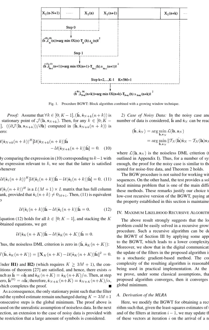
For a slowly varying channel (with respect to the block-size ), the true channel may remain identical during several blocks. This observation suggests that we initialize block with the channel of block . If and are proportional, the vector in block is computed in one iteration. Other-wise, it is crucial to know whether a local minimum of block may also be a local minimum of block since in the latter case, initializing each block with the previous might propa-gate an error from one block to another. We answer partially by providing a necessary and sufficient condition for to be a local minimum different from the global minimum. Based on it, we build a simple numerical test that combines the block algorithm with a growing window technique (the BGWT, cf. Fig. 1).
Block Growing Window Technique (BGWT)
• Step 0: Minimize using the block algorithm (5)
and (6) to obtain .
• Step where : At time , a
new symbol is transmitted. The vector of emitted
symbols is , and its length is . The
minimizer of is (which
is obtained via MLBA).
At the end of these iterations, either for
or , such as . The
consequences of these issues are formalized below.
1) Noiseless Case: The following theorem gives a rule to distinguish the global minimum from the local ones.
Theorem 2: Assume that there is no noise and that the channel is constant over the window
. Assume also that are full column rank matrices for any and
that rank .
If, all along the BGW procedure, and
for any , then
Fig. 1. Procedure BGWT: Block algorithm combined with a growing window technique.
Proof: Assume that is
a stationary point of . Then, for any
computed in is
zero:
(10) By comparing the expression in (10) corresponding to with the expression relevant to , we see that the latter is satisfied whenever
(11) is a matrix that has full column rank, provided that . Then, (11) is equivalent to
(12) Equation (12) holds for all , and stacking the obtained equations, we get
Thus, the noiseless DML criterion is zero in :
Under H1) and H2) (which requires ), the con-ditions of theorem [27] are satisfied, and hence, there exists
such as and . Then, at step
zero, ; therefore, ,
which completes the proof.
As a consequence, the only stationary point such that the filter and the symbol estimate remain unchanged during
consecutive steps is the global minimum. The proof above is based on the unrealistic assumption of noiseless data. In the next section, an extension to the case of noisy data is provided with the restriction that a large amount of symbols is considered.
2) Case of Noisy Data: In the noisy case and if a large number of data is considered, and can be read as
where is the noiseless DML criterion (the proof is outlined in Appendix I). Thus, for a number of symbols large enough, the proof for the noisy case is similar to the proof pre-sented for noise-free data, and Theorem 2 holds.
The BGW procedure is not suited for working with large data sequences. On the other hand, the test provides a solution to the local minima problem that is one of the main difficulties with these methods. These remarks justify our choice to develop a low-cost recursive version of the BGWT, paying attention that the property established in this section is maintained.
IV. MAXIMUMLIKELIHOODRECURSIVEALGORITHM(MLRA) The above result strongly suggests that the local minima problem could be easily solved in a recursive growing window procedure. Such a recursive algorithm can be derived from the BGWT of Section III by applying some approximations to the BGWT, which leads to a lower complexity algorithm. Moreover, we show that in the digital communication context, the update of the filters in the proposed algorithm is equivalent to a stochastic gradient-based method. The computational complexity of the resulting algorithm is reasonably small for being used in practical implementation. At the same time, we prove, under some classical assumptions, that when the proposed algorithm converges, then it converges toward the global minimum.
A. Derivation of the MLRA
Here, we modify the BGWT for obtaining a recursive algo-rithm such that, given the least-squares estimates of the symbols and of the filters at iteration , we may update the estimates of these vectors at iteration on the arrival of a new symbol.
The filters and the symbols are still computed alternately. Let and denote, respectively, the channel and the symbol vector estimated at iteration . The first simplification consists of replacing the minimization in step
of the BGWT by the two relations
(13)
(14) The equations above are quite similar to the equations in the first iteration of step of the BGWT. Equation (13) solves a least-squares problem in , whose length is . Hence, the computational complexity of (13) increases quickly with . Considering that it is unlikely that the most recent re-ceived samples have a strong impact on the estimate of symbols that have been emitted long ago, we update only the last sym-bols. Hence, is a fundamental parameter to be determined, which will drive a complexity/efficiency tradeoff. Implicitly, the other symbols are thus supposed to be correctly estimated. At it-eration is split into two parts:
Updated at iteration .. .
Not updated at and after iteration Now, we consider separately the minimization w.r.t. the symbols and the filter.
1) Minimization With Respect to the Symbols: Since only symbols are updated at iteration , the minimization with respect to the symbols in (13) reduces to
argmin
(15) Matrix can be split into two submatrices:
.. .
(16) By combining (15) and (16), the estimated symbol vector at iteration can be calculated as
(17) where stands for the multiplication operator.
2) Minimization With Respect to the Filter: The filter is obtained using (14). It can be computed recursively from .
Let denote the block
diagonal covariance matrix of the estimated symbols. Then, the update of is performed thanks to
(18) More details on the derivation of this equation is given in Appendix B. The MLRA consists of (17) and (18). Matrix turns out to be a block diagonal matrix with
diag-onal and the
empirical covariance matrix of the estimated symbols. Hence, for , (18) reduces to the classical equations of recursive least-squares (RLS) algorithms (each subchannel being updated separately).
3) Comparison Between the MLRA and the BGWT: The computational complexity of the MLRA is largely reduced compared to the BGWT for the following reasons.
1) The minimization with respect to the joint variable in step of the BGWT (iterative procedure) is replaced by the minimization of a criterion with respect to each vari-able separately, which coincides with the first iteration of step in the BGWT.
2) At iteration , the BGWT computes symbols whose length increases with , whereas only a fixed number (independent of ) symbols are computed in the MLRA. 3) In the MLRA, is updated recursively from ,
which is done without any approximation, whereas, in the BGWT, the whole channel computation is performed in a single step without having any benefit from the channel computations done in the previous steps.
Unfortunately, possible divergence problems may occur. These diverging situations are essentially due to the choice of , which should be greater than (order of the channel). This point is illustrated in Figs. 7 and 8.
B. Initialization
In recursive implementations, the computation usually starts with known initial conditions and makes use of the information contained in the new data samples to update the previous esti-mates. Here, neither the symbols nor the channel are known. Hence, we need to find a reliable initial estimate. A similar problem is encountered in TSML [11] or IQML [12]. Gener-ally, the problem is solved by making use of an initialization procedure such as the subspace algorithm, for example. Here, we propose to initialize the MLRA with defined as the stationary point of the MLBA (5) and (6) over a block of size . The MLBA starts with a randomly chosen ini-tialization point. The choice of reflects a tradeoff between the accuracy of the estimates and the involved computational cost. Experience shows that choosing about leads to a reasonable tradeoff. In any case, this always corresponds to
, which ensures that is the unique global minimum of (cf. Theorem 1).
C. Convergence of the Recursive Algorithm
Our main result concerning the convergence of the MLRA is as follows.
Theorem 3: In the noiseless case, if the MLRA converges, if
H1) and H2) are met, and if situated after the convergence , then the MLRA converges toward the global minimum.
Proof: If the MLRA converges, then such as
and . At iteration , the
estimated filter satisfies the following relation:
(19) Equation (19) is equivalent to
(20) We split the previous expression into two terms, and we obtain
(21)
Since and and
using (19) taken at time , we conclude that the right member of (21) is zero. Then, (21) reduces to
(22) Matrix is full column rank as long as
. Then, we get
(23) Equation (23) holds . We stack the equations obtained
for with , and we obtain
Under H1) and H4), the conditions of Theorem 1 are satisfied; hence, and are the true values of the parameters up to a scalar factor.
Once again, the theorem above, which has been established for noiseless data, can be extended to noisy data with the re-striction that a large amount of data are considered (see Ap-pendix A).
D. Simplified Recursive Algorithm
In the recursive algorithm, the channels are updated thanks to (18), which is equivalent to
(24)
where , and where
diag
blocks
Each block is a matrix. Let denote the el-ement of at line and column ; then,
. We assume that the sequence is
er-godic; then, ,
where is the covariance matrix
of the estimated symbols. We proved (in Section IV-C) that, in the noiseless case, if the recursive algorithm converges, then it converges toward the global minimum. Therefore, for after the
convergence, and , which
leads to
It is generally assumed that is a sequence of i.i.d., com-plex, circular, random variables with zero mean [16]
Note that in the digital communication context, these hy-potheses are most often met [26], [28]. Consequently,
is a diagonal matrix, namely
Therefore, for a time index large enough,
, and . Replacing
the new expression for in (24), we obtain
where . Equation (25) is a member of the stochastic gradient-based algorithms with decreasing step-size parameter (inversely proportional to ) and does not require any longer the inversion of the covariance matrix. In practical situations, this decreasing step strategy should not be used, but the connection with LMS-like algorithms was worth pointing out. It is clear, after these considerations, that LMS-based algorithms will perform very much like RLS-like algorithms.
V. MAXIMUMLIKELIHOODADAPTIVEALGORITHM(MLAA) Adaptivity is an important feature for tracking the variations of time-varying channels, as well as for providing current op-timal solutions, without introducing a large delay due to block processing. The MLAA is obtained by introducing an expo-nential weighting factor into the DML criterion and by writing the corresponding recursions. Under the same assumptions as for the MLRA, it converges toward the global minimum. The MLAA is closely connected with a soft decision feedback equal-izer (SDFE). This link is emphasized at the end of the section. A. Derivation of the MLAA
The adaptivity feature can be obtained by introducing an ex-ponential weighting factor into the definition of the criterion
. Thus, the new criterion can be written
(26)
where . The use of the weighting factor is intended to ensure that data in the distant past is forgotten. Such an algo-rithm is able to track the variations of the channel in a nonsta-tionary environment. Using a matrix formulation,
can be read as
(27) where
diag ... ... ...
We replace with in Section IV-A, and
the MLAA is obtained in the same way as the MLRA. The up-date of the symbols for the MLAA is given by the expression
(28)
As to the update of the filter, we obtain a set of equations that are similar to (18):
(29)
where will
be obtained recursively from . This algorithm will be referred to as the maximum likelihood adaptive algorithm (MLAA). The MLAA also needs a good initialization that is easily obtained by running a block algorithm on a very short window in a manner very similar to the block algorithm of Section III. Arguments very similar to those of Section IV-C can be applied to the MLAA, which prove the following.
i) In the noiseless case and asymptotically in the noisy case, if H1) and H4) are met, if the channel is slowly varying, and if the MLAA converges, then it converges toward the global minimum of the weighted criterion . To the best of our knowledge, this is the first time that we can distinguish the local minima from the global one in that kind of algorithm.
ii) Moreover, is a diagonal matrix, and its diagonal elements are all nonzero. Then, is equivalent to . Therefore, if the previous assumptions are met, the MLAA converges toward the global minimum of . In the case of the MLAA, we do not know . The consequence is that we cannot prove that the MLAA is equiv-alent to a stochastic gradient method. This question will be ad-dressed through simulation in Section VI.
B. Link With an SDFE
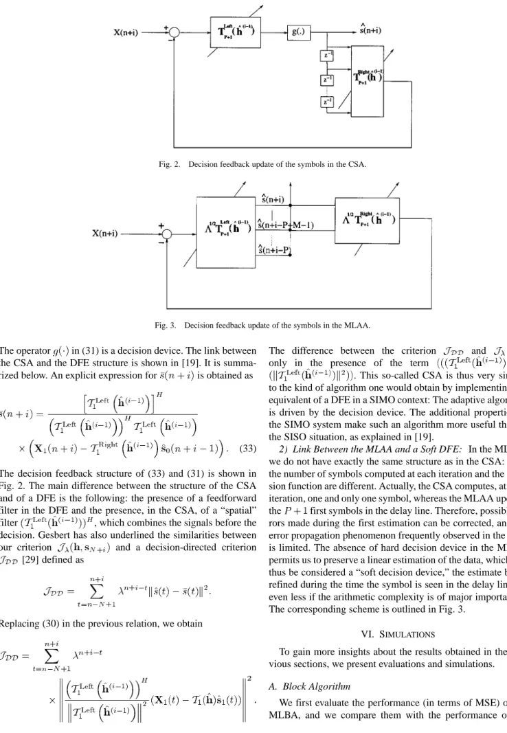
Here, we emphasize that the structure of the MLAA is very close to the structure of an SDFE. In [19], Gesbert has proposed an adaptive algorithm [the channel symbol algorithm (CSA)], based on least-squares techniques that aims at minimizing the criterion (27). We first recall some properties of the CSA.
1) Link Between the CSA and a DFE: For each iteration of the CSA, we have
(30) (31)
Fig. 2. Decision feedback update of the symbols in the CSA.
Fig. 3. Decision feedback update of the symbols in the MLAA. The operator in (31) is a decision device. The link between
the CSA and the DFE structure is shown in [19]. It is summa-rized below. An explicit expression for is obtained as
(33) The decision feedback structure of (33) and (31) is shown in Fig. 2. The main difference between the structure of the CSA and of a DFE is the following: the presence of a feedforward filter in the DFE and the presence, in the CSA, of a “spatial” filter , which combines the signals before the decision. Gesbert has also underlined the similarities between our criterion and a decision-directed criterion
[29] defined as
Replacing (30) in the previous relation, we obtain
The difference between the criterion and lies only in the presence of the term
. This so-called CSA is thus very similar to the kind of algorithm one would obtain by implementing the equivalent of a DFE in a SIMO context: The adaptive algorithm is driven by the decision device. The additional properties of the SIMO system make such an algorithm more useful than in the SISO situation, as explained in [19].
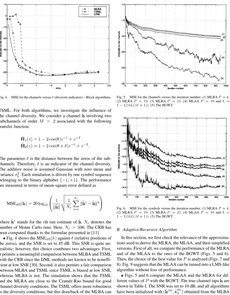
2) Link Between the MLAA and a Soft DFE: In the MLAA, we do not have exactly the same structure as in the CSA: Both the number of symbols computed at each iteration and the deci-sion function are different. Actually, the CSA computes, at each iteration, one and only one symbol, whereas the MLAA updates the first symbols in the delay line. Therefore, possible er-rors made during the first estimation can be corrected, and the error propagation phenomenon frequently observed in the DFE is limited. The absence of hard decision device in the MLAA permits us to preserve a linear estimation of the data, which can thus be considered a “soft decision device,” the estimate being refined during the time the symbol is seen in the delay line (or even less if the arithmetic complexity is of major importance). The corresponding scheme is outlined in Fig. 3.
VI. SIMULATIONS
To gain more insights about the results obtained in the pre-vious sections, we present evaluations and simulations. A. Block Algorithm
We first evaluate the performance (in terms of MSE) of the MLBA, and we compare them with the performance of the
Fig. 4. MSE for the channels versus (diversity indicator)—Block algorithms.
TSML. For both algorithms, we investigate the influence of the channel diversity. We consider a channel involving two subchannels of order associated with the following transfer function:
The parameter is the distance between the zeros of the sub-channels. Therefore, is an indicator of the channel diversity. The additive noise is assumed Gaussian with zero mean and variance . Each simulation is driven by one symbol sequence belonging to the binary alphabet . The performance are measured in terms of mean-square error defined as
MSE
where stands for the th run estimate of . denotes the number of Monte Carlo runs. Here, . The CRB has been computed thanks to the formulae presented in [11].
Fig. 4 shows the MSE against (relative positions of the zeros), and the SNR is set to 45 dB. This SNR is quite un-realistic; however, this choice combines two advantages. First, it permits a meaningful comparison between MLBA and TSML with the CRB since the DML methods are known to be noneffi-cient at low SNR [30]. Second, it also permits a fair comparison between MLBA and TSML since TSML is biased at low SNR, whereas MLBA is not. The simulation shows that the TSML and the MLRA are close to the Cramér-Rao bound for good channel diversity conditions. The TSML offers more robustness to the diversity conditions, but this drawback of the MLBA can be overcome thanks to the introduction of a convex constraint like in [31]. The resulting algorithm is able to estimate the true channels and symbols, even when the subchannels are not co-prime. A full paper is in preparation.
Fig. 5. MSE for the channels versus the iteration number. (1) MLRAP = 4. (2) MLRAP = 10. (3) MLRA P = 25. (4) MLAA P = 10 and =
1 0 1=(6L(M + 1)). (5) The BGWT.
Fig. 6. MSE for the symbols versus the iteration number. (1) MLRAP = 4. (2) MLRAP = 10. (3) MLRA P = 25. (4) MLAA P = 10 and =
1 0 1=(6L(M + 1)). (5) The BGWT.
B. Adaptive/Recursive Algorithm
In this section, we first check the relevance of the approxima-tions used to derive the MLRA, the MLAA, and their simplified versions. First of all, we compare the performance of the MLRA and of the MLAA to the ones of the BGWT (Figs. 5 and 6). Then, the choice of the best value for is analyzed (Figs. 7 and 8). Fig. 9 suggests that the MLAA can be turned into a LMS-like algorithm without loss of performance.
Figs. 5 and 6 compare the MLAA and the MLRA for dif-ferent values of with the BGWT. The true channel taps are shown in Table I. The SNR was set to 10 dB, and all algorithms have been initialized with obtained from the MLBA ran for . The BGWT is optimal since at each iteration, the criterion is minimized, whereas only the first step of the min-imization process is performed in the MLRA. This remark, com-bined with the fact that the MLRA is almost equivalent to the
Fig. 7. MSE for the channels versus SNR obtained with the MLRA for various values ofP .
Fig. 8. MSE for the symbols versus SNR obtained with the MLRA for various values ofP .
LMS algorithm with decreasing stepsize, provides an explana-tion for the growing gap between the MSE of the MLRA and of the BGWT and of the MLAA. Actually, the MLRA has no practical interest, but it was an essential step toward the MLAA. Figs. 5 and 6 show that the MLAA is able to improve the esti-mates with the arrival of new data. Moreover, the simplifications involved in the MLAA lead to small degradations on the perfor-mance.
Figs. 7 and 8 confirm the assumption of Section IV-A dealing with the influence of old symbols on the update of the filters. In this simulation, we compute the MSE on the channels and on the symbols for the MLRA ran for various pairs . We consider the channel described in Table I. The MSE is averaged over 50 Monte Carlo runs (each run corresponds to an independent realization of noise) and is computed at the 1000th iteration. At low SNR and for or , the MLRA diverges for some realizations, which is why the corresponding lines on the figures are incomplete.
Fig. 9. MSE for the channels versus the iteration number obtained for the MLAA and with the simplified MLAA.
TABLE I
IMPULSERESPONSE OFCHANNEL~h
When divergence occurs, the algorithm can be reinitialized by an appropriate procedure, which has not been done in the simulation. Note also that the reason for divergence is strongly linked to a true growing window procedure, which is known to be very sensitive to this kind of problems. Adaptive versions are less sensitive to this phenomenon, as explained below. For and for any SNR, the value of the MSE remains very close to the value obtained when . Here, the order of the channel is . Therefore, the update of the filters seems to be influenced only by the symbols in the delay line of the channels.
Fig. 9 compares the MLAA and the simplified MLAA (SMLAA—LMS-like algorithm) for and
dB. The SMLAA is obtained by replacing in (29) with
the diagonal matrix , where is a
scale factor at iteration between the true parameters and their estimates, and stands for the forgetting factor. The scale factor
is obtained thanks to .
The MSE is averaged over 25 realizations. For each realization, the channel, the symbol sequence, and the noise realization change. In our context, the covariance matrix of the estimated symbols is nearly a diagonal matrix. The proposed simplifica-tion is justified. This is emphasized in Fig. 9.
VII. CONCLUSION
In this paper, three algorithms are proposed to implement DML methods. The MLBA has several desirable properties, including high-SNR consistency, high-SNR efficiency, and a structure suitable for deriving a recursive algorithm. Moreover, a test that permits us to circumvent the local minima problem is provided. A recursive (MLRA) and an adaptive (MLAA)
algorithm based on least-squares techniques are derived. The MLRA follows from various approximations applied to the BGWT. We can remark that both algorithms are strongly con-nected with a RLS. Therefore, fast versions could be obtained using techniques similar as for a fast RLS. Furthermore, the up-date of the filters in the MLRA and the MLAA can be simplified by stochastic gradient techniques. Derivation of the algorithms is straightforward. The MLAA combines several advantages, such as adaptivity, low arithmetic complexity (can be turned into a LMS-like algorithm without loss in the performance), and a DFE-like structure, where the soft decisions limits the error propagation phenomenon, and the local minima can be distinguished from the global minimum (which is unusual with this kind of algorithm). Moreover, the convergence speed of the MLAA can be improved by constraining the symbols into a convex set [31], which will be reported in another paper.
APPENDIX A
DML CRITERION FOR ALARGEAMOUNT OFDATA In the noisy case, the channel and the symbols are estimated through
where . Both and are
de-terministic parameters to be determined, whereas is sto-chastic. Actually, is assumed zero-mean Gaussian with covariance . Asymptotically, in the number of data, we have
where is the mathematical expectation w.r.t. the random variable . Moreover,
can be read
trace .
The term trace is independent of and , and trace
is the noiseless DML criterion. Then, asymptotically (in the number of data), the DML criterion is equivalent to the noiseless DML criterion.
APPENDIX B RECURSIVE COMPUTATION
OF THEFILTER
At iteration verifies the stationary point condition
(34)
We split the covariance matrix of the symbols into two terms in (35), shown at the bottom of the page. The first term will be updated at the next iteration, whereas the second will remain unchanged. Replace by in (34) to obtain a recursive solution for and, thanks to (35), we have
(36)
At iteration , the stationary point condition is
(37)
The product can be expressed
as
(38)
Replacing the previous equations in (36) leads to
Finally, comparing (39) with (34) leads to the update equation for the filters
where . is also
updated recursively:
Then, applying twice the Woodbury’s identity, the recursive equations for the update of is
where is an intermediary matrix.
ACKNOWLEDGMENT
The authors wish to thank the anonymous reviewers for in-sightful comments and helpful suggestions.
REFERENCES
[1] E. de Carvalho and D. Slock, “Semi-blind methods for FIR multichannel estimation,” in Signal Processing Advances in Wireless Communica-tions, Y. Hua, G. B. Giannakis, P. Stoica, and L. Tong, Eds. Englewood Cliffs, NJ: Prentice-Hall, 2000.
[2] D. Hatzinakos and C. Nikias, “Estimation of multipath channel response in frequency selective channels,” IEEE J. Select. Areas Commun., vol. 7, pp. 12–19, Jan. 1989.
[3] J. K. Tugnait, “Blind equalization and estimation of digital communi-cation FIR channels using cumulant matching,” IEEE Trans. Commun., vol. 43, pp. 1240–1245, Feb. 1995.
[4] B. Porat and B. Friedlander, “Blind equalization of digital commu-nication channels using higher-order moments,” IEEE Trans. Signal Prossessing, vol. 39, pp. 522–526, Feb. 1991.
[5] G. B. Giannakis and J. M. Mendel, “Identification of nonminimum phase systems using higher-order-satistics,” IEEE Trans. Acoust., Speech, Signal Processing, vol. 37, pp. 360–377, Mar. 1989.
[6] L. Tong, G. Xu, and T. Kailath, “A new approach to blind identifica-tion and equalizaidentifica-tion of multipath channels,” presented at the Proc. 25th Asilomar Conf, Signals, Syst., Comput., Nov. 1991.
[7] , “Blind identification and equalization based on second-order sta-tistics: A time domain approach,” IEEE Trans. Inform. Theory, vol. 40, pp. 340–349, Mar. 1994.
[8] Y. Li and Z. Ding, “Blind channel identification based on second-order cyclostationary statistics,” in Proc. ICASSP, vol. 4, Apr. 1993, pp. 81–84.
[9] K. Abed-Meraim, E. Moulines, and P. Loubaton, “Prediction error method for second-order blind identification,” IEEE Trans. Signal Processing, vol. 45, pp. 694–705, Mar. 1997.
[10] Y. Hua, H. Yang, and W. Qiu, “Source correlation compensation for blind channel identification based on second-order statistics,” IEEE Signal Processing Lett., vol. 1, pp. 119–120, Aug. 1994.
[11] Y. Hua, “Fast maximum likelihood for blind identification of multiple FIR channels,” IEEE Trans. Signal Processing, vol. 44, pp. 661–672, Mar. 1996.
[12] D. Slock, “Blind fractionaly-spaced equalization, perfect reconstruction filter banks, and multichannel linear prediction,” in Proc. ICASSP, 1994, pp. 585–588.
[13] D. Slock and C. B. Papadias, “Further results on blind identification and equalization of multiple FIR channels,” in Proc. ICASSP, 1995, pp. 1964–1967.
[14] G. Harikuma and Y. Bresler, “Analysis and comparative evaluation of techniques for multichannel blind deconvolution,” Proc. Eighth IEEE Signal Process. Workshop Statist. Signal Array Processing, pp. 332–335, 1996.
[15] C. B. Papadias, “Methods for blind equalization and identification of linear channels,” Ph.D. dissertation, ENST, France, 1995.
[16] L. Tong and S. Perreau, “Multichannel blind identification: From subspace to maximum likelihood methods,” Proc. IEEE, vol. 86, pp. 1951–1968, 1998.
[17] P. Stoica, J. Li, and T. Sderstrm, “On the iconsistency of IQML,” Signal Process., vol. 56, pp. 185–190, July 1997.
[18] J. Ayadi, E. de Carvalho, and D. T. M. Slock, “Blind and semi-blind maximum likelihood methods for FIR multichannel identification,” pre-sented at the ICASSP, WA, May 1998.
[19] D. Gesbert, P. Duhamel, and S. Mayrargue, “Blind least squares criteria for joint data/channel estimation,” presented at the IEEE DSP Work-shop, Sept. 1996.
[20] M. Ghosh and C. L. Weber, “Maximum-likelihood blind equalization,” Opt. Eng., vol. 31, no. 6, pp. 1224–1228, June 1992.
[21] J. Laurila, K. Kopsa, and E. Bonek, “Semi-blind signal estimation for smart antennas using subspace tracking,” in Proc. SPAWC, Annapolis, MD, 1999, pp. 271–274.
[22] E. Pité and P. Duhamel, “Bilinear methods for blind channel equaliza-tion: (No) local minimum issue,” in Proc. ICASSP, May 1998. [23] R. R. Bitmead, S. Y. Kung, B. D. O. Anderson, and T. Kailath, “Greatest
common division via generalized Sylvester and Bezout matrices,” IEEE Trans. Automat. Contr., vol. AC-23, pp. 1043–1047, Dec. 1978. [24] R. E. Blahut, Algebraic Methods for Signal Processing and
[25] L. Ljung, System Identification: Theory for the User. Englewood Cliffs, NJ: Prentice-Hall, 1987.
[26] E. Moulines, P. Duhamel, J. F. Cardoso, and S. Mayrargue, “Subspace methods for the blind identification of multichannel FIR filters,” IEEE Trans. Signal Processing, vol. 43, pp. 516–526, Feb. 1995.
[27] G. Xu and L. Tong, “A deterministic approach to blind channel identi-fication of multi-channel FIR systems,” presented at the ICASSP, Apr. 1994.
[28] M. Gurelli and C. Nikias, “EVAM: An eigenvector-based algorithm for multi-channel blind deconvolution of input colored signals,” IEEE Trans. Signal Processing, vol. 43, pp. 134–149, Jan. 1995.
[29] J. Proakis, Digital Communications. New York: Mc Graw-Hill, 1989. [30] E. de Carvalho and D. T. M. Slock, “Asymptotic performance of ML methods for semi-blind channel estimation,” in Proc. Asilomar Conf. Signals, Syst., Comput., Pacific Grove, CA, Nov. 1997.
[31] F. Alberge, P. Duhamel, and M. Nikolova, “Blind identification/equal-ization using deterministic maximum likelihood and a partial informa-tion on the input,” in Proc. SPAWC, Annapolis, MD, 1999.
Florence Alberge was born in Albi, France, in 1971.
She received the B.E. degree from Ecole Nationale Supérieure de l’Electronique et de ses Applications, Paris, France, and the M.Sc. degree from the Univer-sity of Cergy, Cergy, France, in 1996. She received the Agregation de Physique degree in 1998 and the Ph.D. degree in 1999 from the Ecole Nationale Supérieure des Télécommunications (ENST), Paris.
Since 2000, she has been with the Laboratoire des Signaux et Systèmes, CNRS, Gif sur Yvette, France, and with the University of Paris-Sud, Orsay, France, as an Assistant Professor. Her main research interest is in the field of signal processing for communications.
Pierre Duhamel (F’98) was born in France in
1953. He received the Dipl.-Ing. degree in electrical engineering from the National Institute for Applied Sciences (INSA), Rennes, France, in 1975 and the Dr.-Ing. degree in 1978 and the Doctorat ès sciences degree in 1986, both from Orsay University, Orsay, France.
From 1975 to 1980, he was with Thomson-CSF, Paris, France, where his research interests were in circuit theory and signal processing, including dig-ital filtering and analog fault diagnosis. In 1980, he joined the National Research Center in Telecommunications (CNET), Issy les Moulineaux, France, where his research activities were first concerned with the design of recursive CCD filters. Later, he worked on fast algorithms for computing Fourier transforms and convolutions and applied similar techniques to adaptive filtering, spectral analysis, and wavelet transforms. From 1993 to September 2000, he was a Professor with the National School of Engineering in Telecommunications (ENST), Paris, with research activities focused on signal processing for communications. He was Head of the Signal and Image Pro-cessing Department from 1997 to 2000. He is now with the Laboratoire de Signaux et Systemes, CNRS, Gif sur Yvette, France, where he is developing studies in signal processing for communications (including equalization, itera-tive decoding, and multicarrier systems) and signal/image processing for multi-media applications, including source coding, joint source/channel coding, wa-termarking, and audio processing.
Dr. Duhamel was chairman of the IEEE DSP committee from 1996 to 1998, was an Associate Editor of the IEEE TRANSACTIONS ON SIGNAL
PROCESSINGfrom 1989 to 1991, and was Associate Editor for the IEEE SIGNALPROCESSINGLETTERS. He was a Guest Editor for the special issue of the IEEE TRANSACTIONS ONSIGNALPROCESSINGon wavelets. He is now a member of the Signal Processing for Communications committee. He was an IEEE Distiguished Lecturer for 1999 and was co-general chair of the 2001 International Workshop on Multimedia Signal Processing, Cannes, France. The paper on subspace-based methods for blind equalization, which he co-authored, received the “Best Paper Award” from the IEEE TRANSACTIONS ONSIGNAL
PROCESSINGin 1998. He was awarded the “Grand Prix France Telecom” by the French Science Academy in 2000.
Mila Nikolova received the Ph.D. degree in signal
processing from the Université Paris-Sud, Paris, France, in 1995.
Currently, she is a Researcher with the National Center for Scientific Research (CNRS), Paris. Her re-search interests are in inverse problems and recon-struction of images and signals.