Modern Actuarial Risk Theory

(1)

(2)

Jan Dhaene • Michel Denuit

Theory

Modern Actuarial Risk

Using R

Second Edition

(3)

This work is subject to copyright. All rights are reserved, whether the whole or part of the material is reproduction on microfi lm or in any other way, and storage in data banks. Duplication of this publication

The use of registered names, trademarks, etc. in this publication does not imply, even in the absence of a specifi c statement, that such names are exempt from the relevant protective laws and regulations and therefore free for general use.

Printed on acid-free paper

Cover design: WMXDesign GmbH, Heidelberg UvA / KE

Roetersstraat 11 1018 WB Amsterdam The Netherlands r.kaas@uva.nl

Violations are liable for prosecution under the German Copyright Law. e-ISBN: 978-3-540-70998-5

concerned, specifi cally the rights of translation, reprinting, reuse of illustrations, recitation, broadcasting,

1965, in its current version, and permission for use must always be obtained from Springer-Verlag. or parts thereof is permitted only under the provisions of the German Copyright Law of September 9, Professor Rob Kaas

2nd ed. 2008. Corr. 2nd Printing ISBN: 978-3-642-03407-7 DOI 10.1007/978-3-540-70998-5

Library of Congress Control Number: 2009933607

Springer is part of Springer Science+Business Media (www.springer.com) Springer Heidelberg Dordrecht London New York

Naamsestraat 69 3000 Leuven Belgium

jan.dhaene@econ.kuleuven.be

Faculteit Economie en Bedrijfswetenschappen

Professor Michel Denuit

Belgium

Institut de Statistique K.U. Leuven

Voie du Roman Pays 20 1348 Louvain-la-Neuve Professor Marc Goovaerts

Université Catholique de Louvain AFI (Accountancy, Finance, Insurance) Faculteit Economie en Bedrijfswetenschappen K.U. Leuven Naamsestraat 69 3000 Leuven Belgium Roetersstraat 11 UvA / KE michel.denuit@uclouvain.be 1018 WB Amsterdam The Netherlands marc.goovaerts@econ.kuleuven.be Research Group

AFI (Accountancy, Finance, Insurance)

(4)

Study the past if you would define the future — Confucius, 551 BC - 479 BC

Risk Theory has been identified and recognized as an important part of actuarial ed-ucation; this is for example documented by the Syllabus of the Society of Actuaries and by the recommendations of the Groupe Consultatif. Hence it is desirable to have a diversity of textbooks in this area.

This text in risk theory is original in several respects. In the language of figure skating or gymnastics, the text has two parts, the compulsory part and the free-style part. The compulsory part includes Chapters 1–4, which are compatible with official material of the Society of Actuaries. This feature makes the text also useful to students who prepare themselves for the actuarial exams. Other chapters are more of a free-style nature, for example the chapter on Ordering of Risks, a speciality of the authors. And I would like to mention the chapters on Generalized Linear Models in particular. To my knowledge, this is the first text in risk theory with an introduction to these models.

Special pedagogical efforts have been made throughout the book. The clear lan-guage and the numerous exercises are an example for this. Thus the book can be highly recommended as a textbook.

I congratulate the authors to their text, and I would like to thank them also in the name of students and teachers that they undertook the effort to translate their text into English. I am sure that the text will be successfully used in many classrooms.

Lausanne, 2001 Hans Gerber

(5)

Preface to the Second Edition

When I took office, only high energy physicists had ever heard of what is called the Worldwide Web . . . Now even my cat has its own page — Bill Clinton, 1996

This book gives a comprehensive survey of non-life insurance mathematics. Origi-nally written for use with the actuarial science programs at the Universities of Am-sterdam and Leuven, it is now in use at many other universities, as well as for the non-academic actuarial education program organized by the Dutch Actuarial So-ciety. It provides a link to the further theoretical study of actuarial science. The methods presented can not only be used in non-life insurance, but are also effective in other branches of actuarial science, as well as, of course, in actuarial practice.

Apart from the standard theory, this text contains methods directly relevant for actuarial practice, for example the rating of automobile insurance policies, premium principles and risk measures, and IBNR models. Also, the important actuarial statis-tical tool of the Generalized Linear Models is studied. These models provide extra possibilities beyond ordinary linear models and regression, the statistical tools of choice for econometricians. Furthermore, a short introduction is given to credibil-ity theory. Another topic that always has enjoyed the attention of risk theoreticians is the study of ordering of risks. The book reflects the state of the art in actuarial risk theory; many results presented were published in the actuarial literature only recently.

In this second edition of the book, we have aimed to make the theory even more directly applicable by using the softwareR. It provides an implementation of the language S, not unlike S-Plus. It is not just a set of statistical routines but a full-fledged object oriented programming language. Other software may provide similar capabilities, but the great advantage ofRis that it is open source, hence available to everyone free of charge. This is why we feel justified in imposing it on the users of this book as a de facto standard. On the internet, a lot of documentation aboutR

can be found. In an Appendix, we give some examples of use ofR. After a general introduction, explaining how it works, we study a problem from risk management, trying to forecast the future behavior of stock prices with a simple model, based on stock prices of three recent years. Next, we show how to useRto generate pseudo-random datasets that resemble what might be encountered in actuarial practice.

(6)

Models and paradigms studied

The time aspect is essential in many models of life insurance. Between paying pre-miums and collecting the resulting pension, decades may elapse. This time element is less prominent in non-life insurance. Here, however, the statistical models are generally more involved. The topics in the first five chapters of this textbook are basic for non-life actuarial science. The remaining chapters contain short introduc-tions to other topics traditionally regarded as non-life actuarial science.

1. The expected utility model

The very existence of insurers can be explained by the expected utility model. In this model, an insured is a risk averse and rational decision maker, who by virtue of Jensen’s inequality is ready to pay more than the expected value of his claims just to be in a secure financial position. The mechanism through which decisions are taken under uncertainty is not by direct comparison of the expected payoffs of decisions, but rather of the expected utilities associated with these payoffs.

2. The individual risk model

In the individual risk model, as well as in the collective risk model below, the to-tal claims on a portfolio of insurance contracts is the random variable of interest. We want to compute, for example, the probability that a certain capital will be suf-ficient to pay these claims, or the value-at-risk at level 99.5% associated with the portfolio, being the 99.5% quantile of its cumulative distribution function (cdf). The total claims is modeled as the sum of all claims on the policies, which are assumed independent. Such claims cannot always be modeled as purely discrete random vari-ables, nor as purely continuous ones, and we use a notation, involving Stieltjes inte-grals and differentials, encompassing both these as special cases.

The individual model, though the most realistic possible, is not always very con-venient, because the available dataset is not in any way condensed. The obvious technique to use in this model is convolution, but it is generally quite awkward. Using transforms like the moment generating function sometimes helps. The Fast Fourier Transform (FFT) technique gives a fast way to compute a distribution from its characteristic function. It can easily be implemented inR.

We also present approximations based on fitting moments of the distribution. The Central Limit Theorem, fitting two moments, is not sufficiently accurate in the im-portant right-hand tail of the distribution. So we also look at some methods using three moments: the translated gamma and the normal power approximation. 3. Collective risk models

A model that is often used to approximate the individual model is the collective risk model. In this model, an insurance portfolio is regarded as a process that produces claims over time. The sizes of these claims are taken to be independent, identically distributed random variables, independent also of the number of claims generated. This makes the total claims the sum of a random number of iid individual claim amounts. Usually one assumes additionally that the number of claims is a Poisson variate with the right mean, or allows for some overdispersion by taking a negative

(7)

Preface ix binomial claim number. For the cdf of the individual claims, one takes an average of the cdfs of the individual policies. This leads to a close fitting and computation-ally tractable model. Several techniques, including Panjer’s recursion formula, to compute the cdf of the total claims modeled this way are presented.

For some purposes it is convenient to replace the observed claim severity dis-tribution by a parametric loss disdis-tribution. Families that may be considered are for example the gamma and the lognormal distributions. We present a number of such distributions, and also demonstrate how to estimate the parameters from data. Fur-ther, we show how to generate pseudo-random samples from these distributions, beyond the standard facilities offered byR.

4. The ruin model

The ruin model describes the stability of an insurer. Starting from capital u at time t=0, his capital is assumed to increase linearly in time by fixed annual premiums, but it decreases with a jump whenever a claim occurs. Ruin occurs when the capital is negative at some point in time. The probability that this ever happens, under the assumption that the annual premium as well as the claim generating process remain unchanged, is a good indication of whether the insurer’s assets match his liabili-ties sufficiently. If not, one may take out more reinsurance, raise the premiums or increase the initial capital.

Analytical methods to compute ruin probabilities exist only for claims distribu-tions that are mixtures and combinadistribu-tions of exponential distribudistribu-tions. Algorithms exist for discrete distributions with not too many mass points. Also, tight upper and lower bounds can be derived. Instead of looking at the ruin probabilityψ(u) with initial capital u, often one just considers an upper bound e−Ru for it (Lund-berg), where the number R is the so-called adjustment coefficient and depends on the claim size distribution and the safety loading contained in the premium.

Computing a ruin probability assumes the portfolio to be unchanged eternally. Moreover, it considers just the insurance risk, not the financial risk. Therefore not much weight should be attached to its precise value beyond, say, the first relevant decimal. Though some claim that survival probabilities are ‘the goal of risk theory’, many actuarial practitioners are of the opinion that ruin theory, however topical still in academic circles, is of no significance to them. Nonetheless, we recommend to study at least the first three sections of Chapter 4, which contain the description of the Poisson process as well as some key results. A simple proof is provided for Lundberg’s exponential upper bound, as well as a derivation of the ruin probability in case of exponential claim sizes.

5. Premium principles and risk measures

Assuming that the cdf of a risk is known, or at least some characteristics of it like mean and variance, a premium principle assigns to the risk a real number used as a financial compensation for the one who takes over this risk. Note that we study only risk premiums, disregarding surcharges for costs incurred by the insurance company. By the law of large numbers, to avoid eventual ruin the total premium should be at least equal to the expected total claims, but additionally, there has to be a loading in

(8)

the premium to compensate the insurer for making available his risk carrying capac-ity. From this loading, the insurer has to build a reservoir to draw upon in adverse times, so as to avoid getting in ruin. We present a number of premium principles, together with the most important properties that characterize premium principles. The choice of a premium principle depends heavily on the importance attached to such properties. There is no premium principle that is uniformly best.

Risk measures also attach a real number to some risky situation. Examples are premiums, infinite ruin probabilities, one-year probabilities of insolvency, the re-quired capital to be able to pay all claims with a prescribed probability, the expected value of the shortfall of claims over available capital, and more.

6. Bonus-malus systems

With some types of insurance, notably car insurance, charging a premium based ex-clusively on factors known a priori is insufficient. To incorporate the effect of risk factors of which the use as rating factors is inappropriate, such as race or quite often sex of the policy holder, and also of non-observable factors, such as state of health, reflexes and accident proneness, many countries apply an experience rating system. Such systems on the one hand use premiums based on a priori factors such as type of coverage and list-price or weight of a car, on the other hand they adjust these premiums by using a bonus-malus system, where one gets more discount after a claim-free year, but pays more after filing one or more claims. In this way, premi-ums are charged that reflect the exact driving capabilities of the driver better. The situation can be modeled as a Markov chain.

The quality of a bonus-malus system is determined by the degree in which the premium paid is in proportion to the risk. The Loimaranta efficiency equals the elasticity of the mean premium against the expected number of claims. Finding it involves computing eigenvectors of the Markov matrix of transition probabilities.R

provides tools to do this. 7. Ordering of risks

It is the very essence of the actuary’s profession to be able to express preferences between random future gains or losses. Therefore, stochastic ordering is a vital part of his education and of his toolbox. Sometimes it happens that for two losses X and Y , it is known that every sensible decision maker prefers losing X , because Y is in a sense ‘larger’ than X . It may also happen that only the smaller group of all risk averse decision makers agree about which risk to prefer. In this case, risk Y may be larger than X , or merely more ‘spread’, which also makes a risk less attractive. When we interpret ‘more spread’ as having thicker tails of the cumulative distribu-tion funcdistribu-tion, we get a method of ordering risks that has many appealing properties. For example, the preferred loss also outperforms the other one as regards zero utility premiums, ruin probabilities, and stop-loss premiums for compound distributions with these risks as individual terms. It can be shown that the collective model of Chapter 3 is more spread than the individual model it approximates, hence using the collective model, in most cases, leads to more conservative decisions regarding premiums to be asked, reserves to be held, and values-at-risk. Also, we can prove

(9)

Preface xi that the stop-loss insurance, demonstrated to be optimal as regards the variance of the retained risk in Chapter 1, is also preferable, other things being equal, in the eyes of all risk averse decision makers.

Sometimes, stop-loss premiums have to be set under incomplete information. We give a method to compute the maximal possible stop-loss premium assuming that the mean, the variance and an upper bound for a risk are known.

In the individual and the collective model, as well as in ruin models, we assume that the claim sizes are stochastically independent non-negative random variables. Sometimes this assumption is not fulfilled, for example there is an obvious depen-dence between the mortality risks of a married couple, between the earthquake risks of neighboring houses, and between consecutive payments resulting from a life in-surance policy, not only if the payments stop or start in case of death, but also in case of a random force of interest. We give a short introduction to the risk ordering that applies for this case. It turns out that stop-loss premiums for a sum of random vari-ables with an unknown joint distribution but fixed marginals are maximal if these variables are as dependent as the marginal distributions allow, making it impossible that the outcome of one is ‘hedged’ by another.

In finance, frequently one has to determine the distribution of the sum of de-pendent lognormal random variables. We apply the theory of ordering of risks and comonotonicity to give bounds for that distribution.

We also give a short introduction in the theory of ordering of multivariate risks. One might say that two randoms variables are more related than another pair with the same marginals if their correlation is higher. But a more robust criterion is to restrict this to the case that their joint cdf is uniformly larger. In that case it can be proved that the sum of these random variables is larger in stop-loss order. There are bounds for joints cdfs dating back to Fr´echet in the 1950s and H¨offding in the 1940s. For a random pair(X,Y), the copula is the joint cdf of the ranks FX(X)and

FY(Y). Using the smallest and the largest copula, it is possible to construct random

pairs with arbitrary prescribed marginals and (rank) correlations. 8. Credibility theory

The claims experience on a policy may vary by two different causes. The first is the quality of the risk, expressed through a risk parameter. This represents the aver-age annual claims in the hypothetical situation that the policy is monitored without change over a very long period of time. The other is the purely random good and bad luck of the policyholder that results in yearly deviations from the risk parameter. Credibility theory assumes that the risk quality is a drawing from a certain structure distribution, and that conditionally given the risk quality, the actual claims experi-ence is a sample from a distribution having the risk quality as its mean value. The predictor for next year’s experience that is linear in the claims experience and op-timal in the sense of least squares turns out to be a weighted average of the claims experience of the individual contract and the experience for the whole portfolio. The weight factor is the credibility attached to the individual experience, hence it is called the credibility factor, and the resulting premiums are called credibility

(10)

premiums. As a special case, we study a bonus-malus system for car insurance based on a Poisson-gamma mixture model.

Credibility theory is actually a Bayesian inference method. Both credibility and generalized linear models (see below) are in fact special cases of so-called

General-ized Linear Mixed Models (GLMM), and theRfunctionglmmis able to deal with

both the random and the fixed parameters in these models. 9. Generalized linear models

Many problems in actuarial statistics are Generalized Linear Models (GLM). In-stead of assuming a normally distributed error term, other types of randomness are allowed as well, such as Poisson, gamma and binomial. Also, the expected values of the dependent variables need not be linear in the regressors. They may also be some function of a linear form of the covariates, for example the logarithm leading to the multiplicative models that are appropriate in many insurance situations.

This way, one can for example tackle the problem of estimating the reserve to be kept for IBNR claims, see below. But one can also easily estimate the premiums to be charged for drivers from region i in bonus class j with car weight w.

In credibility models, there are random group effects, but in GLMs the effects are

fixed, though unknown. Theglmmfunction inRcan handle a multitude of models,

including those with both random and fixed effects. 10. IBNR techniques

An important statistical problem for the practicing actuary is the forecasting of the total of the claims that are Incurred, But Not Reported, hence the acronym IBNR, or not fully settled. Most techniques to determine estimates for this total are based on so-called run-off triangles, in which claim totals are grouped by year of origin and development year. Many traditional actuarial reserving methods turn out to be maximum likelihood estimations in special cases of GLMs.

We describe the workings of the ubiquitous chain ladder method to predict future losses, as well as, briefly, the Bornhuetter-Ferguson method, which aims to incorpo-rate actuarial knowledge about the portfolio. We also show how these methods can be implemented inR, using theglmfunction. In this same framework, many exten-sions and variants of the chain ladder method can easily be introduced. England and Verrall have proposed methods to describe the prediction error with the chain ladder method, both an analytical estimate of the variance and a bootstrapping method to obtain an estimate for the predictive distribution. We describe anRimplementation of these methods.

11. More on GLMs

For the second edition, we extended the material in virtually all chapters, mostly

in-volving the use ofR, but we also add some more material on GLMs. We briefly

recapitulate the Gauss-Markov theory of ordinary linear models found in many other texts on statistics and econometrics, and explain how the algorithm by Nelder

and Wedderburn works, showing how it can be implemented inR. We also study

(11)

Preface xiii random variables with a distribution in a subclass of the exponential family. The well-known normal, Poisson and gamma families have a variance proportional to μp_{for p}₌₀_,₁_,_{2, respectively, where}_μ _{is the mean (heteroskedasticity). The}

so-called Tweedie class contains random variables, in fact compound Poisson–gamma risks, having variance proportional toμpfor some p∈(1,2). These mean-variance relations are interesting for actuarial purposes. Extensions toRcontributed by Dunn and Smyth provide routines computing cdf, inverse cdf, pdf and random drawings of such random variables, as well as to estimate GLMs with Tweedie distributed risks.

Educational aspects

As this text has been in use for a long time now at the University of Amsterdam and elsewhere, we could draw upon a long series of exams, resulting in long lists of exercises. Also, many examples are given, making this book well-suited as a text-book. Some less elementary exercises have been marked by[♠], and these might be skipped.

The required mathematical background is on a level such as acquired in the first stage of a bachelors program in quantitative economics (econometrics or actuar-ial science), or mathematical statistics. To indicate the level of what is needed, the book by Bain and Engelhardt (1992) is a good example. So the book can be used either in the final year of such a bachelors program, or in a subsequent masters pro-gram in actuarial science proper or in quantitative financial economics with a strong insurance component. To make the book accessible to non-actuaries, notation and jargon from life insurance mathematics is avoided. Therefore also students in ap-plied mathematics or statistics with an interest in the stochastic aspects of insurance will be able to study from this book. To give an idea of the mathematical rigor and statistical sophistication at which we aimed, let us remark that moment generating functions are used routinely, while characteristic functions and measure theory are avoided in general. Prior experience with regression models, though helpful, is not required.

As a service to the student help is offered, in Appendix B, with many of the exercises. It takes the form of either a final answer to check one’s work, or a useful hint. There is an extensive index, and the tables that might be needed in an exam are printed in the back. The list of references is not a thorough justification with bibliographical data on every result used, but more a collection of useful books and papers containing more details on the topics studied, and suggesting further reading. Ample attention is given to exact computing techniques, and the possibilities that

Rprovides, but also to old fashioned approximation methods like the Central Limit Theorem (CLT). The CLT itself is generally too crude for insurance applications, but slight refinements of it are not only fast, but also often prove to be surprisingly accurate. Moreover they provide solutions of a parametric nature such that one does not have to recalculate everything after a minor change in the data. Also, we want to stress that ‘exact’ methods are as exact as their input. The order of magnitude of errors resulting from inaccurate input is often much greater than the one caused by using an approximation method.

(12)

The notation used in this book conforms to what is usual in mathematical statis-tics as well as non-life insurance mathemastatis-tics. See for example the book by Bowers et al. (1986, 1997), the non-life part of which is similar in design to the first part of this book. In particular, random variables are capitalized, though not all capitals actually denote random variables.

Acknowledgments

First and most of all, the authors would like to thank David Vyncke for all the work he did on the first edition of this book. Many others have provided useful input. We thank (in pseudo-random order) Hans Gerber, Elias Shiu, Angela van Heerwaarden, Dennis Dannenburg, Richard Verrall, Klaus Schmidt, Bjørn Sundt, Vsevolod Ma-linovskii, who translated this textbook into Russian, Qihe Tang, who translated it into Chinese in a joint project with Taizhong Hu and Shixue Cheng, Roger Laeven, Ruud Koning, Pascal Schoenmaekers, Julien Tomas, Katrien Antonio as well as Steven Vanduffel for their comments, and Vincent Goulet for helping us with some

R-problems. Jan Dhaene and Marc Goovaerts acknowledge the support of the Fortis Chair on Financial and Actuarial Risk Management.

World wide web support

The authors would like to keep in touch with the users of this text. On the internet page http://www1.fee.uva.nl/ke/act/people/kaas/ModernART.htm we maintain a list of all typos that have been found so far, and indicate how teachers may obtain solu-tions to the exercises as well as the slides used at the University of Amsterdam for courses based on this book.

To save users a lot of typing, and typos, this site also provides theRcommands used for the examples in the book.

Amsterdam, Rob Kaas

Leuven, Marc Goovaerts

Louvain-la-Neuve, Jan Dhaene

(13)

Chapter 1

Utility theory and insurance

The sciences do not try to explain, they hardly even try to interpret, they mainly make models. By a model is meant a mathematical construct which, with the addition of certain verbal interpretations, describes observed phenomena. The justification of such a mathematical construct is solely and precisely that it is expected to work —

John von Neumann (1903 - 1957)

1.1 Introduction

The insurance industry exists because people are willing to pay a price for being insured. There is an economic theory that explains why insureds are willing to pay a premium larger than the net premium, that is, the mathematical expectation of the insured loss. This theory postulates that a decision maker, generally without being aware of it, attaches a value u(w)to his wealth w instead of just w, where u(·)is called his utility function. To decide between random losses X and Y , he compares E[u(w−X)]with E[u(w−Y)]and chooses the loss with the highest expected util-ity. With this model, the insured with wealth w is able to determine the maximum premium P+he is prepared to pay for a random loss X . This is done by solving the equilibrium equation E[u(w−X)] =u(w−P). At the equilibrium, he does not care, in terms of utility, if he is insured or not. The model applies to the other party in-volved as well. The insurer, with his own utility function and perhaps supplementary

expenses, will determine a minimum premium P−. If the insured’s maximum

pre-mium P+is larger than the insurer’s minimum premium P−, both parties involved increase their utility if the premium is between P−and P+.

Although it is impossible to determine a person’s utility function exactly, we can give some plausible properties of it. For example, more wealth would imply a higher utility level, so u(·)should be a non-decreasing function. It is also logical that ‘reasonable’ decision makers are risk averse, which means that they prefer a fixed loss over a random loss with the same expected value. We will define some classes of utility functions that possess these properties and study their advantages and disadvantages.

Suppose that an insured can choose between an insurance policy with a fixed deductible and another policy with the same expected payment by the insurer and with the same premium. It can be shown that it is better for the insured to choose the former policy. If a reinsurer is insuring the total claim amount of an insurer’s portfolio of risks, insurance with a fixed maximal retained risk is called a stop-loss reinsurance. From the theory of ordering of risks, we will see that this type

(18)

of reinsurance is optimal for risk averse decision makers. In this chapter we prove that a stop-loss reinsurance results in the smallest variance of the retained risk. We also discuss a situation where the insurer prefers a proportional reinsurance, with a reinsurance payment proportional to the claim amount.

1.2 The expected utility model

Imagine that an individual runs the risk of losing an amount B with probability 0.01. He can insure himself against this loss, and is willing to pay a premium P for this insurance policy. If B is very small, then P will be hardly larger than 0.01B. However, if B is somewhat larger, say 500, then P will be a little larger than 5. If B is very large, P will be a lot larger than 0.01B, since this loss could result in bankruptcy. So the premium for a risk is not homogeneous, that is, not proportional to the risk.

Example 1.2.1 (St. Petersburg paradox)

For a price P, one may enter the following game. A fair coin is tossed until a head appears. If this takes n trials, the payment is an amount 2n. Therefore, the expected gain from the game equals∑∞_n₌₁2n(1₂)n=∞. Still, unless P is small, it turns out that very few are willing to enter the game, which means no one merely looks at

expected profits. ∇

In economics, the model developed by Von Neumann & Morgenstern (1947) aims to describe how decision makers choose between uncertain prospects. If a decision maker is able to choose consistently between potential random losses X , then there exists a utility function u(·) to appraise the wealth w such that the decisions he makes are exactly the same as those resulting from comparing the losses X based on the expectation E[u(w−X)]. In this way, a complex decision is reduced to the comparison of real numbers.

For the comparison of X with Y , the utility function u(·)and its linear transform a u(·) +b for some a>0 are equivalent, since they result in the same decision:

E[u(w−X)]≤E[u(w−Y)] if and only if

E[a u(w−X) +b]≤E[a u(w−Y) +b]. (1.1)

So from each class of equivalent utility functions, we can select one, for example by requiring that u(0) =0 and u(1) =1. Assuming u(0)>0, we could also use the utility function v(·)with v(0) =0 and v(0) =1:

v(x) =u(x)−u(0)

u(0) . (1.2)

It is impossible to determine which utility functions are used ‘in practice’. Utility theory merely states the existence of a utility function. We could try to reconstruct a decision maker’s utility function from the decisions he takes, by confronting him

(19)

1.2 The expected utility model 3 with a large number of questions like: “Which premium P are you willing to pay to avoid a loss 1 that could occur with probability q”? Without loss of generality, we take u(0) =0, u(−1) =−1 and initial wealth w=0, by shifting the utility function over a distance w. Then we learn for which value of P we have

u(−P) = (1−q)u(0) +q u(−1) =−q. (1.3) In practice, we would soon experience the limitations of this procedure: the decision maker will grow increasingly irritated as the interrogation continues, and his deci-sions will become inconsistent, for example because he asks a larger premium for a smaller risk or a totally different premium for nearly the same risk. Such mistakes are inevitable unless the decision maker is using a utility function explicitly. Example 1.2.2 (Risk loving versus risk averse)

Suppose that a person owns a capital w and that he values his wealth by the utility function u(·). He is given the choice of losing the amount b with probability 1₂ or just paying a fixed amount1₂b. He chooses the former if b=1, the latter if b=4, and if b=2 he does not care. Apparently the person likes a little gamble, but is afraid of a larger one, like someone with a fire insurance policy who takes part in a lottery. What can be said about the utility function u(·)?

Choose again w=0 and u(0) =0, u(−1) =−1. The decision maker is indifferent between a loss 2 with probability1₂and a fixed loss 1 (b=2). This implies that

u(−1) =u(0) +u(−2)

2 . (1.4)

The function u(·)is neither convex nor concave, since for b=1 and b=4 we get u(−1₂)<u(0) +u(−1)

2 and u(−2)>

u(0) +u(−4)

2 . (1.5)

Note that a function that is convex is often synonymously called ‘concave upward’, a concave function is ‘concave downward’. The connection between convexity of a real function f and convexity of sets is that the so-called epigraph of f , that is, the set of points lying on or above its graph, is a convex set.

Since u(0) =0 and u(−1) =−1, (1.4) and (1.5) yield

u(−2) =−2, u(−1₂)<−1₂ and u(−4)<−4. (1.6) Connecting these five points gives a graph that lies below the diagonal for−1<x<

0 and x<−2, and above the diagonal for x∈(−2,−1). ∇

We assume that utility functions are non-decreasing, although the reverse is con-ceivable, for example in the event of capital levy. Hence, the marginal utility is non-negative: u(x)≥0. The risk averse decision makers are an important group. They have a decreasing marginal utility, so u(x)≤0. Note that we will not be very rigorous in distinguishing between the notions increasing and non-decreasing. If needed, we will use the phrase ‘strictly increasing’. To explain why such

(20)

deci-sion makers are called risk averse, we use the following fundamental theorem (for a proof, see Exercises 1.2.1 and 1.2.2):

Theorem 1.2.3 (Jensen’s inequality)

If v(x)is a convex function and Y is a random variable, then

E[v(Y)]≥v(E[Y]), (1.7)

with equality if and only if v(·)is linear on the support of Y (the set of its possible

values), including the case that Var[Y] =0. ∇

From this inequality, it follows that for a concave utility function

E[u(w−X)]≤u(E[w−X]) =u(w−E[X]). (1.8) Apparently, decision makers with such utility functions prefer to pay a fixed amount E[X]instead of a risky amount X , so they are indeed risk averse.

Now, suppose that a risk averse insured with capital w has the utility function u(·). Assuming he is insured against a loss X for a premium P, his expected utility will increase if

E[u(w−X)]≤u(w−P). (1.9)

Since u(·)is a non-decreasing continuous function, this is equivalent to P≤P+,

where P+ denotes the maximum premium to be paid. This so-called zero utility

premium is the solution to the following utility equilibrium equation

E[u(w−X)] =u(w−P+). (1.10)

The insurer, say with utility function U(·) and capital W , will insure the loss X for a premium P if E[U(W+P−X)]≥U(W), hence P≥P− where P− denotes the minimum premium to be asked. This premium follows from solving the utility equilibrium equation reflecting the insurer’s position:

U(W) =E[U(W+P−−X)]. (1.11)

A deal improving the expected utility for both sides will be possible if P+≥P−. From a theoretical point of view, insurers are often considered to be virtually risk neutral. So for any risk X , disregarding additional costs, a premium E[X]is sufficient. Therefore,

E[U(W+E[X]−X)] =U(W)for any risk X. (1.12)

In Exercise 1.2.3 it is proved that this entails that the utility function U(·)must be linear.

Example 1.2.4 (Risk aversion coefficient)

Given the utility function u(·), how can we approximate the maximum premium P+ for a risk X ?

(21)

1.3 Classes of utility functions 5 Letμ andσ2 _{denote the mean and variance of X . Using the first terms in the} series expansion of u(·)in w−μ, we obtain

u(w−P+)≈u(w−μ) + (μ−P+)u(w−μ);

u(w−X)≈u(w−μ) + (μ−X)u(w−μ) +1₂(μ−X)2u(w−μ). (1.13) Taking expectations on both sides of the latter approximation yields

E[u(w−X)]≈u(w−μ) +1₂σ2u(w−μ). (1.14) Substituting (1.10) into (1.14), it follows from (1.13) that

1 2σ

2

u(w−μ)≈(μ−P+)u(w−μ). (1.15)

Therefore, the maximum premium P+for a risk X is approximately

P+≈μ−1₂σ2u

₍_w₋_μ₎

u(w−μ). (1.16)

This suggests the following definition: the (absolute) risk aversion coefficient r(w) of the utility function u(·)at wealth w is given by

r(w) =−u

₍_w₎

u(w). (1.17)

Then the maximum premium P+to be paid for a risk X is approximately

P+≈μ+1₂r(w−μ)σ2. (1.18)

Note that r(w)does not change when u(·)is replaced by a u(·)+b. From (1.18), we see that the risk aversion coefficient indeed reflects the degree of risk aversion: the

more risk averse one is, the larger the premium one is willing to pay. ∇

1.3 Classes of utility functions

Besides the linear functions, other families of suitable utility functions exist that have interesting properties:

linear utility: u(w) =w

quadratic utility: u(w) =−(α−w)2 (w≤α) logarithmic utility: u(w) =log(α+w) (w>−α) exponential utility: u(w) =−αe−αw (α>0)

power utility: u(w) =wc (w>0,0<c≤1)

(22)

These utility functions, and of course their linear transforms as well, have a non-negative and non-increasing marginal utility; for the quadratic utility function, we set u(w) =0 if w>α. The risk aversion coefficient for the linear utility function is 0, while for the exponential utility function, it equalsα. For the other utility functions, it can be written as(γ+βw)−1for someγandβ, see Exercise 1.3.1.

Note that linear utility leads to the principle of equivalence and risk neutrality (net premiums), since if E[w+P−−X] =w, then P−=E[X].

Example 1.3.1 (Exponential premium)

Suppose that an insurer has an exponential utility function with parameterα. What is the minimum premium P−to be asked for a risk X ?

Solving the equilibrium equation (1.11) with U(x) =−αe−αx_yields

P−= 1

αlog(mX(α)), (1.20)

where mX(α) =E[eαX]is the moment generating function of X at argumentα. We

observe that this exponential premium is independent of the insurer’s current wealth W , in line with the risk aversion coefficient being a constant.

The expression for the maximum premium P+is the same as (1.20), see Exercise 1.3.3, but now of courseαrepresents the risk aversion of the insured. Assume that the loss X is exponentially distributed with parameterβ. Takingβ =0.01 yields E[X] =_β1=100. If the insured’s utility function is exponential with parameterα= 0.005, then P+= 1 αlog(mX(α)) =200 log _β β−α =200 log(2)≈138.6, (1.21) so the insured is willing to accept a sizable loading on the net premium E[X]. ∇

The approximation (1.18) from Example 1.2.4 yields

P+≈E[X] +₂1αVar[X] =125. (1.22)

Obviously, the approximation (1.22) is increasing with α, but also the premium

(1.20) is increasing if X is a non-negative random variable with finite variance, as we will prove next.

Theorem 1.3.2 (Exponential premium increases with risk aversion)

The exponential premium (1.20) for a risk X is an increasing function of the risk aversionα.

Proof. For 0<α<γ, consider the strictly concave function v(·)with

v(x) =xα/γ. (1.23)

From Jensen’s inequality, it follows that

(23)

1.3 Classes of utility functions 7 for any random variable Y with Var[Y]>0. Take Y=eγX_{, then v}₍_Y_{) =}_eαX _and

E[eγX]α=(E[Y])α/γγ=v(E[Y])γ>E[v(Y)]γ=E[eαX]γ. (1.25) Therefore,

{mX(α)}γ<{mX(γ)}α, (1.26)

which implies that, for anyγ>α, for the exponential premiums we have 1

αlog(mX(α))<1

γlog(mX(γ)). (1.27)

So the proof is completed. ∇

Just as for the approximation (1.18), the limit of (1.20) asα ↓0 is the net pre-mium. This follows immediately from the series expansion of log(mX(t)), see also

Exercise 1.3.4. But asα↑∞, the exponential premium tends to max[X], while the approximation goes to infinity.

Example 1.3.3 (Quadratic utility)

Suppose that for w<5, the insured’s utility function is u(w) =10w−w2_{. What is} the maximum premium P+as a function of w, w∈[0,5], for an insurance policy against a loss 1 with probability1₂? What happens to this premium if w increases?

Again, we solve the equilibrium equation (1.10). The expected utility after a loss X equals

E[u(w−X)] =11w−11₂ −w2, (1.28)

and the utility after paying a premium P equals

u(w−P) =10(w−P)−(w−P)2. (1.29)

By the equilibrium equation (1.10), the right hand sides of (1.28) and (1.29) should be equal, and after some calculations we find the maximum premium as

P=P(w) =11₂ −w2+1₄−(5−w), w∈[0,5]. (1.30) One may verify that P(w)>0, see also Exercise 1.3.2. We observe that a deci-sion maker with quadratic utility is willing to pay larger premiums as his wealth increases toward the saturation point 5. Because of this property, quadratic utility is less appropriate to model the behavior of risk averse decision makers. The quadratic utility function still has its uses, of course, since knowing only the expected value

and the variance of the risk suffices to do the calculations. ∇

Example 1.3.4 (Uninsurable risk)

A decision maker with an exponential utility function with risk aversionα>0 wants to insure a gamma distributed risk with shape parameter n and scale parameter 1. See Table A. Determine P+and prove that P+>n. When is P+=∞and what does that mean?

(24)

P+= 1

αlog(mX(α)) = − n

αlog(1−α)for 0<α<1

∞ forα≥1. (1.31)

Since log(1+x)<x for all x>−1, x=0, we have also log(1−α)<−α and con-sequently P+>E[X] =n. So the resulting premium is larger than the net premium. Ifα ≥1, then P+=∞, which means that the decision maker is willing to pay any finite premium. An insurer with risk aversionα ≥1 insuring the risk will suffer a loss, in terms of utility, for any finite premium P, since also P−=∞. For such

insurers, the risk is uninsurable. ∇

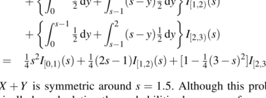
Remark 1.3.5 (Allais paradox (1953), Yaari’s dual theory (1987)) Consider the following possible capital gains:

X= 1 000 000 with probability 1 Y = ⎧ ⎨ ⎩ 5 000 000 with probability 0.10 1 000 000 with probability 0.89 0 with probability 0.01 V = 1 000 000 with probability 0.11 0 with probability 0.89 W = 5 000 000 with probability 0.10 0 with probability 0.90

Experimental economy has revealed that, having a choice between X and Y , many people choose X , but at the same time they prefer W over V . This result violates the expected utility hypothesis, since, assuming an initial wealth of 0, the latter pref-erence E[u(W)]>E[u(V)]is equivalent to 0.11 u(1 000 000)<0.1 u(5 000 000)+ 0.01 u(0), but the former leads to exactly the opposite inequality. Apparently, ex-pected utility does not always describe the behavior of decision makers adequately. Judging from this example, it would seem that the attraction of being in a completely safe situation is stronger than expected utility indicates, and induces people to make irrational decisions.

Yaari (1987) has proposed an alternative theory of decision making under risk that has a very similar axiomatic foundation. Instead of using a utility function, Yaari’s dual theory computes ‘certainty equivalents’ not as expected values of trans-formed wealth levels (utilities), but with distorted probabilities of large gains and losses. It turns out that this theory leads to paradoxes that are very similar to the

ones vexing utility theory. ∇

1.4 Stop-loss reinsurance

Reinsurance treaties usually do not cover the risk fully. Stop-loss (re)insurance cov-ers the top part. It is defined as follows: for a loss X , assumed non-negative, the payment is

(25)

1.4 Stop-loss reinsurance 9 1 0 d x FX fX(x)

{

Area = (x-d)fX(x)

Fig. 1.1 Graphical derivation of (1.33) for a discrete cdf.

(X−d)+:=max{X−d,0}= X−d if X>d;

0 if X≤d. (1.32)

The insurer retains a risk d (his retention) and lets the reinsurer pay for the remain-der, so the insurer’s loss stops at d. In the reinsurance practice, the retention equals the maximum amount to be paid out for every single claim and d is called the pri-ority. We will prove that, regarding the variance of the insurer’s retained loss, a stop-loss reinsurance is optimal. The other side of the coin is that reinsurers do not offer stop-loss insurance under the same conditions as other types of reinsurance. Theorem 1.4.1 (Net stop-loss premium)

Consider the stop-loss premium, by which we mean the net premiumπX(d):=

E[(X−d)₊] for a stop-loss contract. Both in the discrete case, where FX(x)is a

step function with a step fX(x)in x, and in the continuous case, where FX(x)has

fX(x)as its derivative, the stop-loss premium is given by

πX(d) = ⎧ ⎨ ⎩ ∑x>d(x−d)fX(x) _∞ d(x−d)fX(x)dx ⎫ ⎬ ⎭= _∞ d [1−FX(x)]dx. (1.33)

Proof. This proof can be given in several ways. A graphical ‘proof’ for the discrete case is given in Figure 1.1. The right hand side of the equation (1.33), that is, the total shaded area enclosed by the graph of FX(x), the horizontal line at 1 and the vertical

line at d, is divided into small bars with a height fX(x)and a width x−d. Their total

area equals the left hand side of (1.33). The continuous case can be proved in the same way by taking limits, considering bars with an infinitesimal height.

(26)

E[(X−d)+] = _∞ d ( x−d)fX(x)dx =−(x−d)[1−FX(x)] ∞ d + ∞ d [1−FX(x)]dx. (1.34)

Note that we do not just take FX(x)as an antiderivative of fX(x). The only choice

FX(x)+C that is a candidate to produce finite terms on the right hand side is FX(x)−

1. With partial integration, the integrated term often vanishes, but this is not always easy to prove. In this case, for x→∞this can be seen as follows: since E[X]<∞, the integral₀∞t fX(t)dt is convergent, and hence the ‘tails’ tend to zero, so

x[1−FX(x)] =x _∞ x fX(t)dt≤ _∞ x t fX(t)dt↓0 for x→∞. (1.35)

In many cases, easier proofs result from using Fubini’s theorem, that is, swapping the order of integration in double integrals, taking care that the integration is over the same set of values inR2_{. In this case, we have only one integral, but this can} be fixed by writing x−d=_dxdy. The pairs(x,y)over which we integrate satisfy d<y<x<∞, so this leads to _∞ d (x−d)fX(x)dx= _∞ d x d dy fX(x)dx= _∞ d _∞ y fX(x)dx dy = ∞ d [1−FX(y)]dy. (1.36)

By the same device, the proof in the discrete case can be given as

∑

x>d (x−d)fX(x) =

∑

x>d _x d dy fX(x) = _∞ d x

∑

>y fX(x)dy= _∞ d [ 1−FX(y)]dy. (1.37)

Note that in a Riemann integral, we may change the value of the integrand in a countable set of arguments without affecting the outcome of the integral, so it does

not matter if we take∑_x≥yfX(x)or∑x>yfX(x). ∇

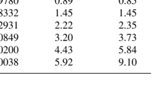
Theorem 1.4.2 (Stop-loss transform)

The functionπX(d) =E[(X−d)+], called the stop-loss transform of X , is a

con-tinuous convex function that is strictly decreasing in the retention d, as long as FX(d)<1. When FX(d) =1,πX(d) =0, and alwaysπX(∞) =0. If X is non-negative,

thenπX(0) =E[X], and for d<0,πX(d)decreases linearly with slope−1.

Proof. From (1.33), it follows that: π

X(d) =FX(d)−1. (1.38)

Since FX(x) =Pr[X ≤x], each cdf FX is continuous from the right. Accordingly,

the derivative in (1.38) is a right hand derivative. Since FX(x)is non-decreasing,

(27)

1.4 Stop-loss reinsurance 11

μ

Fig. 1.2 A stop-loss transformπX(d)for a risk X≥0 with E[X] =μ.

FX(d)<1. If X is non-negative, thenπX(d) =E[(X−d)+] =E[X−d] =E[X]−d

for d≤0. That lim_d→∞πX(d) =0 is evident. These properties are illustrated in

Figure 1.2. ∇

In the next theorem, we prove the important result that a stop-loss insurance mini-mizes the variance of the retained risk.

Theorem 1.4.3 (Optimality of stop-loss reinsurance)

Let I(X)be the payment on some reinsurance contract if the loss is X , with X≥0. Assume that 0≤I(x)≤x holds for all x≥0. Then

E[I(X)] =E[(X−d)+] =⇒Var[X−I(X)]≥Var[X−(X−d)+]. (1.39)

Proof. Because of the previous theorem, for every I(·)we can find a retention d such that the expectations E[I(X)]and E[(X−d)₊]are equal. We write the retained risks as follows:

V(X) =X−I(X) and W(X) =X−(X−d)+. (1.40)

Since E[V(X)] =E[W(X)], it suffices to prove that

E[{V(X)−d}2]≥E[{W(X)−d}2]. (1.41) A sufficient condition for this to hold is that|V(X)−d| ≥ |W(X)−d|with proba-bility one. This is trivial in the event X≥d, since then W(X)≡d holds. For X<d, we have W(X)≡X , and hence

V(X)−d=X−d−I(X)≤X−d=W(X)−d<0. (1.42)

(28)

The essence of the proof is that stop-loss reinsurance makes the risk ‘as close to d’ as possible, under the retained risks with a fixed mean. So it is more attractive because it is less risky, more predictable. As stated before, this theorem can be extended: using the theory of ordering of risks, one can prove that stop-loss insurance not only minimizes the variance of the retained risk, but also maximizes the insured’s expected utility, see Chapter 7.

In the above theorem, it is crucial that the premium for a stop-loss coverage is the same as the premium for another type of coverage with the same expected payment. Since the variance of the reinsurer’s capital will be larger for a stop-loss coverage than for another coverage, the reinsurer, who is without exception at least slightly risk averse, in practice will charge a higher premium for a stop-loss insurance. Example 1.4.4 (A situation in which proportional reinsurance is optimal) To illustrate the importance of the requirement that the premium does not depend on the type of reinsurance, we consider a related problem: suppose that the insurer collects a premium(1+θ)E[X]and that he is looking for the most profitable rein-surance I(X)with 0≤I(X)≤X and prescribed variance

Var[X−I(X)] =V. (1.43)

So the insurer wants to maximize his expected profit, under the assumption that the instability of his own financial situation is fixed in advance. We consider two methods for the reinsurer to calculate his premium for I(X). In the first scenario (A), the reinsurer collects a premium(1+λ)E[I(X)], structured like the direct insurer’s. In the second scenario (B), the reinsurer determines the premium according to the variance principle, which means that he asks as a premium the expected value plus a loading equal to a constant, sayα, times the variance of I(X). Then the insurer can determine his expected profit, which equals the collected premium less the expected value of the retained risk and the reinsurance premium, as follows:

A : (1+θ)E[X]−E[X−I(X)]−(1+λ)E[I(X)]

=θE[X]−λE[I(X)];

B : (1+θ)E[X]−E[X−I(X)]−(E[I(X)] +αVar[I(X)])

=θE[X]−αVar[I(X)].

(1.44)

As one sees, in both scenarios the expected profit equals the original expected profit θE[X]reduced by the expected profit of the reinsurer. Clearly, we have to minimize the expected profit of the reinsurer, hence the following minimization problems A and B arise:

A : Min E[I(X)] B : Min Var[I(X)]

s.t. Var[X−I(X)] =V s.t. Var[X−I(X)] =V (1.45)

To solve Problem B, we write

(29)

1.4 Stop-loss reinsurance 13

(

μ

(d)

,σ

(d))

0 σ μ

I

(

.

)

d= ∞ d=0

Fig. 1.3 Expected value and standard deviation of the retained risk for different reinsurance con-tracts. The boundary line constitutes the stop-loss contracts with d∈[0,∞). Other feasible reinsur-ance contracts are to be found in the shaded area.

Since the first two terms on the right hand side are given, the left hand side is mini-mal if the covariance term is maximized. This can be accomplished by taking X and X−I(X)linearly dependent, choosing I(x) =γ+βx. From 0≤I(x)≤x, we find γ=0 and 0≤β≤1; from (1.43), it follows that(1−β)2₌_V_/_Var_[_X_]_{. So, if the} variance V of the retained risk is given and the reinsurer uses the variance principle, then proportional reinsurance I(X) =βX withβ=1−V/Var[X]is optimal.

For the solution of problem A, we use Theorem 1.4.3. By calculating the deriva-tives with respect to d, we can prove that not just μ(d) =E[X−(X−d)+], but alsoσ2(d) =Var[X−(X−d)+]is continuously increasing in d. See Exercise 1.4.3. Notice thatμ(0) =σ2(0) =0 andμ(∞) =μ=E[X],σ2(∞) =σ2=Var[X].

In Figure 1.3, we plot the points(μ(d),σ(d))for d∈[0,∞)for some loss random variable X . Because of Theorem 1.4.3, other reinsurance contracts I(·)can only have an expected value and a standard deviation of the retained risk above the curve in theμ,σ2-plane, since the variance is at least as large as for the stop-loss reinsurance with the same expected value. This also implies that such a point can only be located to the left of the curve. From this we conclude that, just as in Theorem 1.4.3, the non-proportional stop-loss solution is optimal for problem A. The stop-loss contracts in this case are Pareto-optimal: there are no other solutions with both a smaller variance

(30)

1.5 Exercises

For hints with the exercises, consult Appendix B. Also, the index at the end of the book might be a convenient place to look for explanations.

Section 1.2

1. Prove Jensen’s inequality: if v(x)is convex, then E[v(X)]≥v(E[X]). Consider especially the case v(x) =x2_.

2. Also prove the reverse of Jensen’s inequality: if E[v(X)]≥v(E[X])for every random variable X, then v is convex.

3. Prove: if E[v(X)] =v(E[X])for every random variable X, then v is linear.

4. A decision maker has utility function u(x) =√x, x≥0. He is given the choice between two random amounts X and Y , in exchange for his entire present capital w. The probability distribu-tions of X and Y are given by Pr[X=400] =Pr[X=900] =0.5 and Pr[Y=100] =1−Pr[Y= 1600] =0.6. Show that he prefers X to Y . Determine for which values of w he should decline the offer. Can you think of utility functions with which he would prefer Y to X?

5. Prove that P−≥E[X]for risk averse insurers.

6. An insurer undertakes a risk X and after collecting the premium, he owns a capital w=100. What is the maximum premium the insurer is willing to pay to a reinsurer to take over the complete risk, if his utility function is u(w) =log(w)and Pr[X=0] =Pr[X=36] =0.5? Find not only the exact value, but also the approximation (1.18) of Example 1.2.4.

7. Assume that the reinsurer’s minimum premium to take over the risk of the previous exercise equals 19 and that the reinsurer has the same utility function. Determine his capital W . 8. Describe the utility function of a person with the following risk behavior: after winning an

amount 1, he answers ‘yes’ to the question ‘double or quits?’; after winning again, he agrees only after a long huddle; the third time he says ‘no’.

9. Verify that P+[2X]<2P+[X]when w=0, X∼Bernoulli(1/2) and u(x) = ⎧ ⎪ ⎨ ⎪ ⎩ 2x/3 for x>−3/4, 2x+1 for−1<x<−3/4, 3x+2 for x<−1. Section 1.3

1. Prove that the utility functions in (1.19) have a non-negative and non-increasing marginal utility. Show how the risk aversion coefficient of all these utility functions can be written as r(w) = (γ+βw)−1_.

2. Show that, for quadratic utility, the risk aversion increases with the capital. Check (1.28)– (1.30) and verify that P(w)>0 in (1.30).

3. Prove the formula (1.20) for P−for the case of exponential utility. Also show that (1.10) yields the same solution for P+.

4. Prove that the exponential premium P− in (1.20) decreases to the net premium if the risk aversionαtends to zero.

(31)

1.5 Exercises 15 5. Show that the approximation in Example 1.2.4 is exact if X∼N(μ,σ2₎_{and u}₍_·₎_{is exponential.} 6. Using the exponential utility function withα=0.001, determine which premium is higher: the one for X∼N(400,25 000)or the one for Y∼N(420,20 000). Determine for which values ofαthe former premium is higher.

7. Assume that the marginal utility of u(w)is proportional to 1/w, that is, u(w) =k/w for some k>0 and all w>0. What is u(w)? With this utility function and wealth w=4, show that only prices P<4 in the St. Petersburg paradox of Example 1.2.1 make entering the game worthwhile.

8. It is known that the premium P that an insurer with exponential utility function asks for a N(1000,1002₎_{distributed risk satisfies P}_≥_{1250. What can be said about his risk aversion}_α_? If the risk X has dimension ‘money�