A Study on the Effect of Surface Finish on Corrosion of Carbon Steel in CO2 Environment

(1)

A Study on the Effect of Surface Finish on Corrosion of Carbon Steel in CO2 Environment

by

Nor Asma Rusni Ab. Alim

Dissertation submitted in partial fulfilment of the requirements for the

Bachelor of Engineering (Hons) (Mechanical Engineering)

JULY 2008

Universiti Teknologi PETRONAS

Bandar Seri Iskandar

31750 Tronoh

(2)

CERTIFICATION OF APPROVAL

A STUDY ON THE EFFECT OF SURFACE FINISH ON CORROSION OF CARBON STEEL IN CO2 ENVIRONMENT

by

Nor Asma Rusni Ab. Alim

A project dissertation submitted to the Mechanical Engineering Programme

Universiti Teknologi PETRONAS in partial fulfilment of the requirement for the

BACHELOR OF ENGINEERING (Hons) (MECHANICAL ENGINEERING)

Approved by,

______________________ (Ir. Dr. Mokhtar Che Ismail)

UNIVERSITI TEKNOLOGI PETRONAS

TRONOH, PERAK

(3)

CERTIFICATION OF ORIGINALITY

This is to certify that I am responsible for the work submitted in this project, that the original work is my own except as specified in the references and acknowledgements, and that the original work contained herein have not been undertaken or done by unspecified sources or persons.

____________________________ (NOR ASMA RUSNI AB. ALIM)

(4)

ABSTRACT

Standard surface finish used in laboratory corrosion testing may not represent the „as-delivered‟ internal pipe surface condition, which typically varies from 20 µm to 50 µm. Surface roughness is known to affect the hydrodynamic and mass-transfer boundary layer, thus influencing the corrosion mechanism and rate. The objective of this study is to investigate the effect of various grit surface finishes of 60, 240, 400, 600, 800 and 1200 used in laboratory corrosion testing in predicting field corrosion behaviour.

The effect of the surface roughness on the corrosion rate is investigated by varying the specimen surface finishing using SiC abrasive paper of 60, 240, 400, 600, 800 and 1200 grit. The specimen used is carbon steel BS 970 (070M20), tested in stagnant and turbulent CO2 environment at pH 5.5 and 3 wt% NaCl. The corrosion

rate is measured by the Linear Polarization Resistance (LPR) Long Term and Custom Sweep, Weight Loss and Electrochemical Impedance Spectroscopy (EIS) method.

Surface profiles produced by 400, 600 and 800 grit samples fall within the range of 20 µm to 50 µm, which resemble the „as-delivered‟ internal pipe surface roughness. Corrosion rates in turbulent flow are higher than static condition for all surface finish. For both static condition and turbulent flow, the average corrosion rates of 400, 600 and 800 grit finish samples obtained differ within 18% and 15%, respectively.

In conclusion, based on surface profiles and corrosion rate measured, the practice of 400, 600 and 800 grit surface finish in laboratory testing is acceptable to represent the „as-delivered‟ pipe condition.

(5)

ACKNOWLEDGEMENT

My sincere appreciation goes to:

1. My supervisor, Ir. Dr. Mokhtar Che Ismail for his guidance and advice throughout the study.

2. Laboratory technicians and graduate assistants at Building 17 for the helps and guidance in conducting the experiments.

3. Universiti Teknologi PETRONAS for the opportunity.

4. Friends and family for their invaluable support.

(6)

LIST OF ABBREVIATIONS

CO2 Carbon Dioxide

EIS Electrochemical Impedance Spectroscopy LPR Linear Polarisation Resistance

NaCl Sodium Chloride

SEM Scanning Electron Microscopy

LIST OF FIGURES

Figure 1 Effect of NaCl Concentration on Corrosion Rate of Iron in Aerated Room-temperature Solutions

Figure 2 Pipe Roughness versus Maximum Flow Rate Figure 3 Schematic of Experiment Preparations Figure 4 Experimental Set-Up for Static Test Figure 5 Experimental Set-Up for Dynamic Test

Figure 6 Corrosion Rate (mm/year) for Different Surface Finishes at Static Condition (LPR -LT) Figure 7 Average Corrosion Rate (mm/year) for Different Surface Finishes at Static Condition

(LPR -LT)

Figure 8 Corrosion Rate (mm/year) for Different Surface Finishes at 1000 rpm (LPR - LT)

Figure 9 Average Corrosion Rate (mm/year) for Different Surface Finishes at 1000 rpm (LPR - LT) Figure 10 Comparison of Average Corrosion Rate between Static and 1000 rpm at Different Surface

Finishes (LPR - LT)

Figure 11 Average Corrosion Rate (mm/year) for Different Surface Finishes (LPR - CS) Figure 12 Corrosion Rate (mm/year) for Different Surface Finishes (Weight Loss) Figure 13 Corrosion Rate (mm/year) for Different Surface Finishes (EIS)

Figure 14 Nyquist Plot for Different Surface Finishes at Static Condition Figure 15 Nyquist Plot for Different Surface Finishes at 1000 rpm

LIST OF TABLES

Table 1 European/USA Equivalency Grit Guide

Table 2 Advantages and Disadvantages of RCE Table 3 Surface Profiles for Different Surface Finishes Table 4 Steel Specifications for BS 970 (070M20)

Table 5 Corrosion Rate (mm/year) for Different Surface Finishes at Static Condition (LPR -LT) Table 6 Corrosion Rate (mm/year) for Different Surface Finishes at 1000 rpm (LPR - LT) Table 7 Average Corrosion Rate (mm/year) for Different Surface Finishes at Static Condition

(LPR – CS)

Table 8 Average Corrosion Rate (mm/year) for Different Surface Finishes at 1000 rpm (LPR - CS) Table 9 Weight Loss (g) and Corrosion Rate (mm/year) for Different Surface Finishes

(9)

CHAPTER 1 INTRODUCTION

1.1 Background of Study

The impact of corrosion failures in the oil and gas industry not only can be related to the health, safety and environment (HSE), but also on the capital and operational expenditures (CAPEX and OPEX). Thus, managing corrosion is often an important part of an overall design philosophy. The main motivation behind a corrosion study always lies in the desire to optimise the life cycle cost and ensure technical integrity of facilities in an industry.

In most cases, the prediction of field corrosion behaviour is derived from the laboratory test results. For example, empirical predictive models for carbon steel in CO2 environment such as deWaard and Milliams are based on best-fit parameters

from experimental results. However, the experimental results do not always successfully reproduce the field corrosion condition [1], which gives rise to argument on its reliability and accuracy.

One of the attributing factors that might cause the difference is the surface roughness of the sample used in laboratory. While it is ideal to reproduce the „as-delivered‟ surface roughness in laboratory test, such condition is usually not possible as the field equipments may vary as fabricated and has interacted with its operating environment. In laboratory practice, a commonly used surface finishing is the 800 grit. The question of the 800 grit finish to represent the „as-delivered‟ surface condition is valid.

Thus, the aim of this study is to investigate the effects of various surface finishes representing the „as-delivered‟ surface roughness on CO2 corrosion of carbon steel.

(10)

1.2 Problem Statement

Standard surface finish used in laboratory corrosion testing may not represent the „as-delivered‟ internal pipe surface condition, which typically varies from 20 µm to 50 µm. Surface roughness is known to affect the hydrodynamic and mass-transfer boundary layer, thus influencing the corrosion mechanism and rate. This can be due to lack of specific conduct for specimen surface finishing and the failure to reproduce the „as-delivered‟ roughness condition in laboratory tests.

1.3 Significance of Study

The difference in surface roughness of the „as-delivered‟ condition with that produced in laboratory by sandpaper polishing may cause inaccuracy or failure to reproduce the field corrosion condition. Hence, this study can help to clarify the gap between the differences in surface roughness and increase the reliability of corrosion predictions in laboratory tests.

1.4 Objectives and Scope of Study

The objectives of this study are as follow:

1) To study the effect of 60, 240, 400, 600, 800 and 1200 grit surface finishing on CO2 corrosion rates at pH 5.5 and 3 wt% NaCl of carbon steel under stagnant

and turbulent flow condition.

2) To investigate and compare the above corrosion rates by employing the LPR long term and custom sweep, EIS and weight loss method.

(11)

CHAPTER 2 BACKGROUND THEORY AND LITERATURE REVIEW

2.1 CO2 Corrosion

Carbon dioxide (CO2) is by far the most prevalent attack encountered in upstream

operations. CO2 corrosion or „sweet corrosion‟ of carbon steels was first recorded in

the U.S. oil and gas industry in 1940s. The first significant CO2 corrosion model was

introduced by deWaard and Milliams [2] in 1975, identifying the combined effect of CO2 partial pressure and temperature on the corrosion rate. Since then, many

researches and prediction models on CO2 corrosion has been conducted.

Dry CO2 gas is not corrosive at the temperatures encountered in most productions,

but its presence in aqueous phase results in weak acid and promotes an electrochemical reaction between the steel and the contacting aqueous phase.Oxygen dissolves in formation or condensed water to form weak acid:

The increase of corrosion rate with CO2 can be associated with the increase of

hydrogen evolution reaction. The rate determining step is due to the H+ diffusion rate from the solution. De Waard and Milliams [2] proposed that in carbon acid solution (4<pH<6), direct reduction of carbonic acid becomes the dominant cathodic reaction:

2H2CO3 + 2e-  H2 + 2HCO3

-CO2 (aq) + H2O  H2CO3 (carbonic acid)

H2CO3  H+ + HCO3- (bicarbonate)

(12)

The presence of dissolved CO2 species concentrations in solution and the mass

transport of dissolved CO2 to the steel surface have a critical influence on the

reaction and subsequent rate [3] and that every dissolved species present in the media can contribute to the cathodic reaction. Another important feature of CO2

corrosion is the formation of a protective film that is affected by other parameters such as surface roughness, temperature, flow and pH.

2.2 The Effect of NaCl Presence on Corrosion Rate

Salt, also scientifically known as sodium chloride (NaCl) or halite, is a white crystalline solid and occurs naturally in seawater, underground deposits and brine wells. Salt content of formation water varies dependent upon the location and widely came across in upstream operations.

In presence of salt, the corrosion problem is associated with the significant chloride ions (Cl-) and the operating environments. This combined effect results from the fact that chloride ions in solution can be incorporated into and penetrate surface corrosion films which can lead to destabilization of the corrosion film and lead to increased corrosion.

Many researches have been done at lower salt content (typically up to 3 wt %), and no significant effects of salt concentration on general CO2 corrosion are observed in

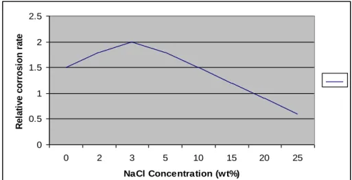
this range [4]. Uhlig and Revie [5] have conducted a research on effect of NaCl concentration on corrosion rate of iron in aerated room-temperature solutions, and concluded that the corrosion rate is highest at 3 wt%, as shown by the subsequent figure. This experiment is conducted with 3 wt% NaCl to simulate the worst case condition.

(13)

0 0.5 1 1.5 2 2.5 0 2 3 5 10 15 20 25 NaCl Concentration (wt%) R e la ti v e c orr os ion r a te

Figure 1: Effect of NaCl Concentration on Corrosion Rate of Iron in Aerated Room-temperature Solutions

2.3 Literature Review of Surface Roughness

Surface roughness plays an important role in determining how an object will interact with its environment. Rough surfaces usually wear more quickly and have higher friction coefficients than smooth surfaces. Grit, Mesh and Micron are generally the three different ways to measure particle size that defines the coarseness of a surface. Surface roughness is usually expressed as Ra parameter, the arithmetic average of the peak-to-valley height of surface asperities in micrometers (μm).

Ideally, in laboratory test, the surface of the specimen should be identical with the surface of actual equipment to be investigated. However, this is usually not possible as the surfaces of field equipment vary as fabricated and due to its interaction nature with environment.

Laboratory test practice standards for corrosion measurement such as NACE and ASTM emphasize on the reproducibility of the results by removing a substantial layer of metal from the test specimens to eliminate variations of the original metallic surface conditions. However, the lack of specific conduct and guidelines to what surfacefinish should be employed leads to variations in surface roughness which can affect the corrosion rate measurement, since different surface finish produces different surface roughness.

(14)

According to NACE [6], a common and widely used surface finish is produced by polishing with No. 120 abrasive paper or its equivalent. This is not a smooth surface, but it is also not rough, and it can be readily produced. However, Fontana [7] proposed that a smoother surface finish up to 800 grit may be required in certain cases, especially when low corrosion rates are anticipated.

The subsequent table shows the guide for European/USA Equivalency Grit. Midpoints for the size ranges for the ANSI/CAMI graded paper according to ANSI standard B74.18 – 1996 and FEPA graded paper standard 43-GB-1984 (R1993).

Table 1: European/USA Equivalency Grit Guide

FEPA (Europe) ANSI/CAMI (USA)

Grit Number Size(μm) Grit Number Size(μm)

P60 269.0 60 268.0 P80 201.0 80 188.0 P100 162.0 100 148.0 P120 127.0 120 116.0 P180 78.0 180 78.0 P240 58.5 220 66.0 P280 52.2 240 51.8 P320 46.2 P360 40.5 280 42.3 P400 35.0 320 34.3 P500 30.2 360 27.3 P600 25.8 P800 21.8 400 22.1 P1000 18.3 500 18.2 P1200 15.3 600 14.5 P1500 12.6 800 12.2 P2000 10.3 1000 9.2 P2500 8.4 1200 6.5 P4000 5.0

A number of studies have been carried out to investigate various aspects of surface roughness in relation to the corrosion rate. Cheng and Roscoe [8] investigated the influence of surface polishing on the electrochemical behaviour of titanium. The research concluded that, contrary to the common belief that a smooth surface will give a higher corrosion resistance, at high anodic potential range (>2.0 V), the 1 µm diamond paste polished electrode gave a much higher anodic current than the rough

(15)

sandpaper polished ones, indicating a less protective passive film formed on the diamond paste polished electrode surface compared to that polished with the sandpaper.

Klein et al [9] investigated the erosion/corrosion resistance of chromium nickel steel in the “as-delivered” condition and the surface roughness of the heat treated version in a multiphase CO2 corrosion. The results indicate that one of the heat treated

versions of the steel has higher wear resistance.

Corrosion studies by their very nature involve an examination of the surface that has been interacted with environment. According to Fogg and Morse [10], steel pipe delivered to the coating yard has a relative roughness in order of 20 μm, and may exceed 50 μm, depending on the corrosion products formed on the surface due to the amount of time and conditions the pipe was stored in prior to installation, hydrostatic testing, and the corrosion nature of the fluid being tested. In such cases, localized metal dissolution is involved, and the surface would become non uniformly roughened.

This in turn affects the fluids in motion, which are subjected to various frictional resistances. Friction occurs between the fluid and the pipeline wall, and also within the fluid. Some of the main factors affecting fluid flow include [10]:

 The length, internal diameter, and internalroughness of the pipe

 The geometry of the pipeline

 The viscosity, density and velocity of the fluid

 Changes in fluid temperature

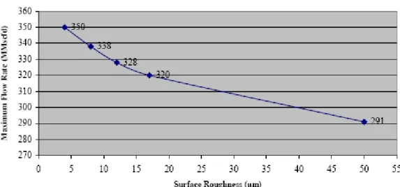
Fogg and Morse [10] have also done a research in 2005 on the effect of surface roughness on the maximum flow rate of a subsea gas export line as given in the subsequent figure:

(16)

Figure 2: Pipe Roughness versus Maximum Flow Rate

It can be seen that the maximum flow rate decreases with increasing internal surface roughness. Turbulent flow of natural gas transportation in pipelines can form a laminar film at the pipe wall – fluid interface, which will reduce the friction between the fluid and pipe wall. Creation of this laminar film is dependent on the surface roughness at the pipe wall – fluid interface, fluid velocity and extent of turbulent flow.

Increased roughness would affect the hydrodynamic boundary layer, mass-transfer boundary layer, thus affecting the fluid-velocity sensitive corrosion mechanism.

(17)

CHAPTER 3 METHODOLOGY

3.1 Time Frame

The Final Year Project (FYP) is structured to be completed in 2 semesters. FYP I carry 2 credit hours and is aimed at gathering information and completing the literature review of the intended project. The experiments and result interpretations are carried out during FYP II which carries 4 credit hours.

The proposed time frame for this study is included in Appendix 1.

3.2 Corrosion Rate Measurement

In this study, the corrosion rate is measured as millimeters per year (mm/year) by employing the weight loss and electrochemical polarization methods.

Polarization is an electrochemical phenomenon where electrode reactions are assumed to induce deviations from equilibrium due to the passage of an electrical current through an electrochemical cell, causing a change in the working electrode potential [11].

The electrochemical polarization methods involving small perturbations are:

 Linear Polarization Resistance (LPR)

(18)

3.2.1 Linear Polarization Resistance (LPR)

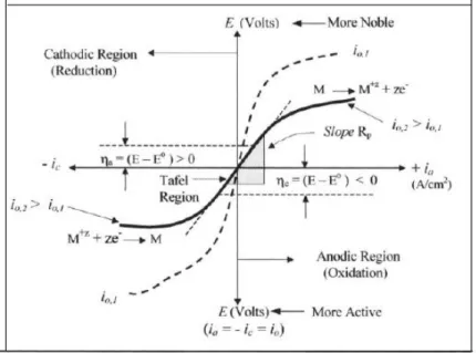
LPR is based on the linear approximation of the polarization behaviour at potentials near the corrosion potential. This steady-state method defines the polarization resistance of a material as the slope of the potential – current density (ΔE / Δi) curves at the free corrosion potential [12], yielding the polarization resistance, Rp.

The schematic of the linear polarization curve is shown in the subsequent figure.

Figure 3.2.1: Schematic Linear Polarization Curve

The linear polarization is confined to a small magnitude of overpotentials of ήa and ήc, respectively, using linear coordinates. The Stern-Geary constant, B, is approximated as 25 mV for all pH. The technique allows the determination of icorr

using a potential range of + 10 mV from the Ecorr . Rp can be calculated from:

The rate of the corrosion then can be calculated from Faraday‟s law:

Corrosion rate (mm / year) =

where:

 Rp = polarisation resistance

 icorr = corrosion current density

 B = 25mV

315 x Z x icorr

ρ x n x F B ΔE

icorr Δi ΔE_ 0

(19)

To improve reliability of the results, LPR test is carried out on the Long Term basis (corrosion rate measurement over one hour) and also Custom Sweep (instantaneous rate measured in one minute).

3.2.2 Electrochemical Impedance Spectroscopy (EIS)

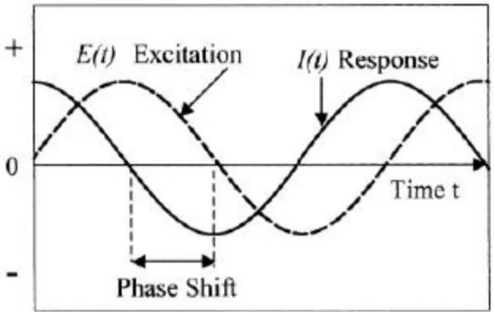
EIS is based on a transient response of an equivalent circuit for an electrode/solution interface. In impedance method, a sine-wave perturbation of small amplitude is employed on a corroding system being modeled as an equivalent circuit for determining the corrosion mechanism and the polarization resistance.

Figure 3.2.2: Schematic Potential Sinusoidal Excitation

The impedance of the system can be calculated as a function of frequency using Ohm‟s Law as:

In addition, Ohm‟s Law can be viewed in two different current imposition cases as per ASTM G-106 standard testing method:

where:

Z = atomic weight of iron, 56 g/mol icorr = corrosion current density ρ = density of iron, 7.8 g/cm3

F = Faraday‟s constant, 96 500 C/mole n = no of electrons lost

(20)

In modeling electrochemical system as an electrochemical circuit, a potential waveform is applied across the circuit and a current response to the frequency signals generates impedance data. icorr can be determined from:

Similar to LPR, the corrosion rate is then calculated from Faraday‟s Law.

3.2.3 Weight Loss Method

Prior to exposure to similar corrosive environment for 7 days, the samples will be cleaned and weighed. After the exposure period, the samples will be cleansed with deionized water and rust remover to remove the corrosion products with minimum removal of sound metal. Then, the specimen is dried and weighed again to record the mass loss due to corrosion. By assuming general corrosion, the corrosion rate is determined form the equation [6]:

Corrosion rate (mm/year) =

3.3 Rotating Cylinder Electrode (RCE)

When troubleshooting a field corrosion problem, researchers often need to return to laboratory and reproduce the similar harsh conditions s in a controlled setting. RCE is a relatively cheap and simpler way to simulate a fluid flow condition compared to laboratoryoratory flow loop systems which require complex and expensive plumbing, maintenance and calibration.

Fluid flow is one of main factor that accelerates corrosion. Even though mathematically, RCE has been proven to generate similar environment with the real

mass loss x 87.6 area x time x metal density

(21)

conditions, there are still many debates among researchers about its quality to simulate the effect of flow in real condition. Efird [12] suggested the advantages and disadvantages of RCE include:

Table 2: Advantages and Disadvantages of RCE

Advantages Disadvantages

Equations for mass transfer and wall shear stress well defined

Wall shear stress > 300 Pa is difficult to achieve

Fully developed wall shear stress is uniform over the entire surface

Testing is single phase liquid only for the equations to apply

Electrochemical tests, electrical resistance probes and coupons can be used

Maintaining good electrical contact with the rotating electrodes is difficult

Easy to use with no pumps or valves required

Testing under high pressure is difficult

3.3.1 Modelling Pipeline Flow Using RCE

A critical issue arise upon simulating a field corrosion condition is choosing the proper rotation rate at which to perform the electrochemical measurement. Silverman [13] proposed that the two approaches that have received attention are:

1. Equality of Wall Shear Stress,

2. Equality of Mass Transfer Coefficients;

which are measured between the RCE and the geometry being modeled. For fully turbulent flow, the two methods are linked because of the relationship that exists between the friction factor and the mass transfer coefficient. The geometry modeled in this study is the straight pipe.

3.3.1.1 Mass Transfer Coefficient Equality

When the rate of mass transfer is the rate controlling step in the corrosion process, the corrosion rate can, in theory, be calculated from the product of the mass transfer coefficient for that geometry and environment, and the difference in concentration of the rate-limiting species between that which is at the surface and that which is in the

(22)

environment [14]. In this experiment, in order to simulate the same conditions between the pipe and RCE, the mass transfer coefficient will be set equal by adjusting the RCE rotation rates using the following equation [13]:

The wall shear stress for RCE can be determined from the Eisenberg Equation:

Silverman [13] also proposed that under some conditions, both mass transfer coefficients and fluid shear stresses could be simultaneously similar between the RCE and pipes, but this may require alterations to the RCE diameter.

3.4 Surface Profiling

The surface finish of the rod-shaped carbon steel specimen is created by attaching it to a rotating cylinder at 100 rpm while grinded. Rotational grinding is performed at the surface by using SiC sandpaper 60, 240, 400, 600, 800 and 1200grit. Deionised water and ethanol is used as the lubricant, to produce a range of different surface roughness. Prior to the roughness verification using surface profiler, the grinded specimen is rinsed with deionised water and ethanol and dried.

The Mitutoyo Surface Profiler measures the roughness as Ra and Rz parameter, the arithmetic average and depth of the peak-to-valley height of surface asperities in micrometers (μm). The equipment has a sensitivity of 250 μm. An average of six random readings is taken, as shown in the subsequent table:

Table 3: Surface Profiles for Different Surface Finishes Surface

Profile

Surface Finish (grit)

60 240 400 600 800 1200 Average Ra (μm) 8.45 13.03 25.56 22.78 20.07 15.87 Average Rz (μm) 38.02 26.56 22.01 21.96 19.98 18.95 2 3 . 0

Re

0791

.

0

_cyl cyl

U









4 5 0657 . 0 7 3 25 . 0

₍

₎

_]

)

[(

1185

.

0

2 8 5 pipe pipe cyl cyl

Sc

U

d

U









(23)

Based on the surface profiles, it can be said that the 400 and 600 grit finish can best represent the „as-delivered‟ condition, which according to Fogg and Morse [10], have a relative roughness of 20 μm to 50 μm.

The surface profiles and SEM imaging for each surface finishing can be found in

Appendix 2 and Appendix3.

3.5 Experiment Preparations and Set-ups

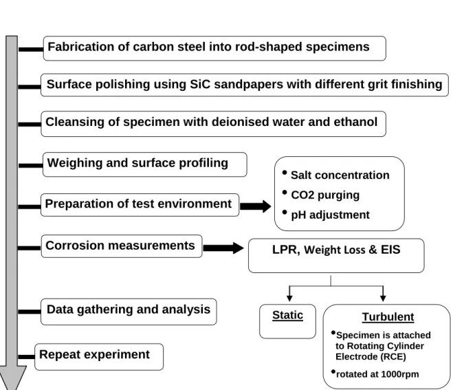
Figure 3: Schematic of Experiment Preparations

•

Salt concentration

•

CO2 purging

•

pH adjustment

Fabrication of carbon steel into rod-shaped specimens

Surface polishing using SiC sandpapers with different grit finishing Cleansing of specimen with deionised water and ethanol

Weighing and surface profiling

Preparation of test environment

Corrosion measurements

Data gathering and analysis

Repeat experiment Static _Turbulent

•

Specimen is attached to Rotating Cylinder Electrode (RCE)

•

rotated at 1000rpm

(24)

3.5.1 Static Test

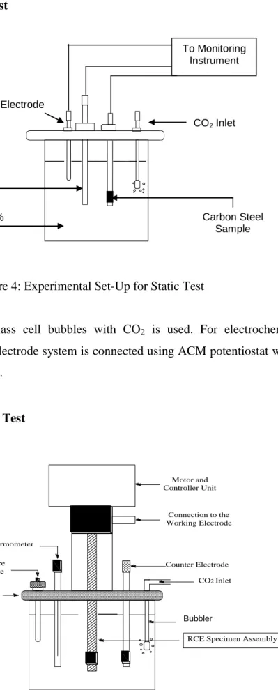
Figure 4: Experimental Set-Up for Static Test

A standard one-litre glass cell bubbles with CO2 is used. For electrochemical

measurements, a three-electrode system is connected using ACM potentiostat with a computer control system.

3.5.2 Dynamic Test To Monitoring Instrument Carbon Steel Sample CO2 Inlet Auxiliary Electrode Reference Electrode Electrolyte 3wt% NaCl, pH 5.5 Cell Lid Reference Electrode Thermometer

RCE Specimen Assembly Bubler CO2 Inlet Counter Electrode Connection to the Working Electrode Motor and Controller Unit Bubbler

(25)

Figure 5: Experimental Set-Up for Dynamic Test

The electrode system and apparatus is similar to static test, except for the specimen is attached to the RCE and rotated at 1000 rpm for turbulent flow.

During experiments, to ensure result reproducibility, test samples and solutions will be prepared accurately and experiment is repeated twice for each case. The NaCl solution is saturated by CO2 by purging for at least 30 minutes prior to the exposure

of electrode. The pH of the solution is adjusted by adding certain amount of 1M NaHCO3.

3.5.3 Test Matrix

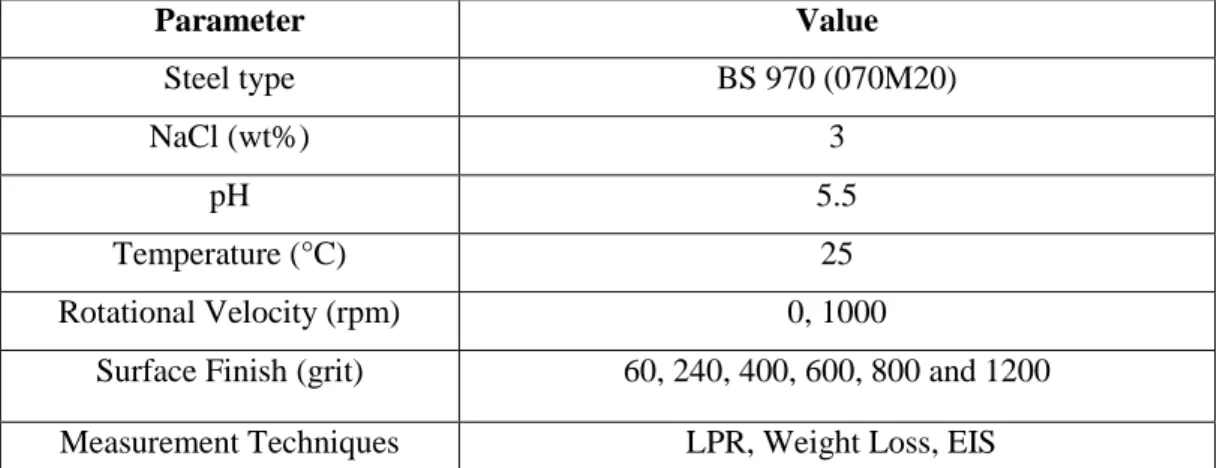
The corrosion evaluations in this study will be performed under stagnant and dynamic conditions, with the use of static electrodes and RCE apparatus. The subsequent test matrix will be applied:

Parameter Value Steel type BS 970 (070M20) NaCl (wt%) 3 pH 5.5 Temperature (°C) 25 Rotational Velocity (rpm) 0, 1000

Surface Finish (grit) 60, 240, 400, 600, 800 and 1200

Measurement Techniques LPR, Weight Loss, EIS

3.6 Material

The electrochemical experiments under both static and dynamic conditions will be conducted with carbon steel type BS 970 (070M20). The BS 970 code number system is constructed as follows [15]:

(26)

i) The first three symbols are a number code indicating the type of steel. 000 to 199 are carbon and carbon-manganese steels. The number represents manganese content x 100.

ii) The fourth symbol is a letter code „M‟ which indicates that the steel is supplied to a Mechanical Property specification.

iii) The fifth and sixth symbol is a number that shows the mean carbon content x 100.

The table below shows the properties of the steel:

Table 4: Steel Specifications for BS 970 (070M20) Type of Steel BS 970 Spec Composition % C-Mn-Ni-Cr-Mo Condition Yield Stress (MPa) Tensile Stress (MPa) Elongation (%) Low carbon steel 070M20 0.2%C 0.7%Mn Normalized 215 430 21

The carbon steel sample is fabricated in rod shape and has the following dimension:

Internal diameter : 6.40 mm External diameter : 11.87 mm Length : 8.05 mm Exposure Area : 3 .00 cm3

(27)

CHAPTER 4 RESULTS & DISCUSSION

4.1 LPR (Long Term) Test Result

In static condition, the effect of various surface finishes on the corrosion rate of carbon steel in 3 wt% NaCl with CO2 at pH 5.5, tested at 25 °C, is shown in Table 5:

Table 5: Corrosion Rate (mm/year) for Different Surface Finishes at Static Condition (LPR -LT)

Time (min)

Surface Finish (Grit)

60 240 400 600 800 1200 0 1.2 2.1 1.4 3.6 1.8 2.7 5 1.2 2.4 1.4 3.1 1.7 2.4 10 1.1 2.3 1.4 2.7 1.7 1.8 15 1.1 2.1 1.5 2.6 1.7 1.5 20 1.2 2.1 1.4 2.5 1.8 1.5 25 1.2 2.1 1.5 2.4 1.6 1.5 30 1.2 2.1 1.5 2.3 1.8 1.5 35 1.2 2.1 1.4 2.3 1.7 1.5 40 1.2 2.0 1.4 2.1 1.7 1.5 45 1.2 2.0 1.4 2.0 2.0 1.4 50 1.2 2.1 1.4 2.0 1.7 1.5 55 1.2 2.0 1.5 2.0 1.7 1.4 60 1.2 2.0 1.4 2.0 1.7 1.5 Average 1.2 2.1 1.4 2.3 1.7 1.5

The trend of the corrosion rates with respect to the surface finishes used in shown in Figure 6:

(28)

Corrosion Rate vs Time 0 0.5 1 1.5 2 2.5 3 3.5 4 0 5 10 15 20 25 30 35 40 45 50 55 60 Time (min) C orr os ion R a te ( m m /y e a r) 60 240 400 600 800 1200

Figure 6: Corrosion Rate (mm/year) for Different Surface Finishes at Static Condition (LPR -LT)

The corrosion rates are found to be steady after the 10th minute. Therefore, the average corrosion rate is taken from the 10th minute onwards and can be depicted by Figure 7:

Average Corrosion Rate vs Surface Finish

0 0.5 1 1.5 2 2.5 60 240 400 600 800 1200 Surface Finish (Grit)

A v e ra ge C orr os ion R a te (m m /y e a r) avrg CR

Figure 7: Average Corrosion Rate (mm/year) for Different Surface Finishes at Static Condition (LPR -LT)

(29)

The average corrosion rate for static condition is highest at 600 grit, which is 2.3 mm/year and lowest at 60 grit, differ by 1.1 mm/year. The worst case scenario can be seen at 600 grit finishing. Corrosion rate does not vary much among the surface finishes at static condition and is thus insignificant.

The effect of various surface finishes on the corrosion rate of carbon steel in 3 wt% NaCl with CO2 at pH 5.5, tested at 25 °C in turbulent flow, is shown in Table 6:

Table 6: Corrosion Rate (mm/year) for Different Surface Finishes at 1000 rpm (LPR - LT)

Time (min)

60 240 400 600 800 1200 0 2.8 6.0 4.0 4.0 4.7 6.2 5 1.9 4.3 3.0 2.8 1.7 0.8 10 1.5 4.3 2.5 2.5 1.3 0.9 15 1.5 4.1 2.3 2.2 1.3 1.0 20 1.4 3.3 2.2 2.1 1.0 0.7 25 1.0 3.0 2.0 2.0 1.4 0.7 30 1.0 2.9 2.0 1.9 1.5 0.7 35 1.0 2.5 1.8 1.9 1.6 0.5 40 1.2 2.9 1.8 1.8 1.6 0.5 45 1.0 2.9 1.8 1.7 1.7 0.5 50 1.1 2.8 1.7 1.7 1.3 0.6 55 1.0 2.7 1.7 1.6 1.5 0.6 60 1.0 2.7 1.6 1.6 1.3 0.6 Average 1.2 3.1 1.9 1.9 1.4 0.7

(30)

Corrosion Rate vs Time 0 1 2 3 4 5 6 7 0 5 10 15 20 25 30 35 40 45 50 55 60 Time (min) C orr os ion R a te ( m m /y e a r) 60 240 400 600 800 1200

Figure 8: Corrosion Rate (mm/year) for Different Surface Finishes at 1000 rpm (LPR - LT)

The average corrosion rate which is taken from the 10th minute onwards, where the rates are stable can be depicted by the Figure 9:

0 0.5 1 1.5 2 2.5 3 3.5 60 240 400 600 800 1200

A v e ra ge C orr os ion R a te (m m /y e a r) avrg CR

Figure 9: Average Corrosion Rate (mm/year) for Different Surface Finishes at 1000 rpm (LPR - LT)

The average corrosion rate obtained varies at different surface finish. The highest corrosion rate is 3.1 mm/year, observed at 240 grit surface finish, while the rate is lowest at 1200 grit. The difference between the highest and lowest rate is 2.4 mm/year. It is observed that the average corrosion rate at 400 grit and 600 grit is similar.

(31)

In comparison, the average corrosion rate taken from 10th minute onwards for both static and 1000 rpm can be represented by Figure 10:

0 0.5 1 1.5 2 2.5 3 3.5 60 240 400 600 800 1200

A v e ra ge C orr os ion R a te (m m /y e a r) 1000rpm static

Figure 10: Comparison of Average Corrosion Rate between Static and 1000 rpm at Different Surface Finishes (LPR - LT)

At 400 grit finish, the turbulent condition shows higher corrosion rate than that of static. But the result is vice versa at 600 grit. The corrosion rate at 240 grit is quite unusual as the value jumps abruptly from that of other surface finishes. Therefore, it is predicted that there were errors during the experiment was conducted. One of the most possible errors is that the surface of specimen has large and significant scratches on the surface that results from insufficient lubricant during polishing. If the prediction of error is true, then the worst case scenarios are showed by 400 and 600 grit finishes.

As such, 400 and 600 grit surface finishes in laboratory can be used to represent the „as-delivered‟ surface roughness in turbulent flow. The practice of 800 grit finish is also acceptable as the difference is relatively small. The trends obtained by LPR Long Term are to be compared with other methods below.

4.2 LPR (Custom Sweep) Test Result

Similar test was conducted by using LPR Custom Sweep. The average of two corrosion rate readings was recorded, as shown in Table 7 and 8:

(32)

Table 7: Average Corrosion Rate (mm/year) for Different Surface Finishes at Static Condition (LPR - CS)

Reading

60 240 400 600 800 1200

1 1.2 1.0 1.0 1.0 1.2 1.0

2 1.0 0.9 0.9 0.8 0.6 0.7

Average 1.1 1.0 1.0 0.9 0.9 0.9

Table 8: Average Corrosion Rate (mm/year) for Different Surface Finishes at 1000 rpm (LPR - CS)

Reading

60 240 400 600 800 1200

1 1.8 1.5 1.2 1.5 1.2 1.1

2 1.4 1.4 1.6 1.2 1.3 0.7

Average 1.6 1.5 1.4 1.4 1.3 0.9

The trend of the above data can be represented by Figure 11:

0 0.2 0.4 0.6 0.8 1 1.2 1.4 1.6 1.8 60 240 400 600 800 1200 Surface Finish (grit)

A v e ra ge C orr os in R a te (m m /y e a r) 1000rpm static

Figure 11: Average Corrosion Rate (mm/year) for Different Surface Finishes (LPR - CS)

The graph indicates that the corrosion rate decreases as finer surface is used. In turbulent flow, the highest corrosion rate is at 60 grit which is 1.6 mm/year, while the lowest rate is 0.9 mm/year at 1200 grit. This gives a difference of 0.7 mm/year.

(33)

Figure 11 also shows that at 1000 rpm, 400 and 600 grit surface finishes yield similar corrosion rate. The corrosion rate at 800 grit is slightly less than that of 400 and 600 grit. The trend of these results agrees with that obtained with LPR Long Term.

In static condition, the highest corrosion rate is 1.1 mm/year at 60 grit. The lowest reading is recorded as 0.9 mm/year at 1200 grit. The difference is 0.2 mm/year. At all surface finishes, the corrosion rate at turbulent flow is higher than that of static condition.

4.3 Weight Loss Test Result

The density of carbon steel measured in laboratory is 7.91 g/cm3. The specimen is exposed for 7 days which is equivalent to 168 hours and the area of specimen is 3 cm2. The corrosion rate in mm/year is measured by [6]:

Corrosion rate (mm/year) =

where mass loss is in mg, area in cm2, time is the hours of exposure and density in g/cm3. Table 9 shows the results of the weight loss and corrosion rate obtained:

Table 9: Weight Loss (g) and Corrosion Rate (mm/year) for Different Surface Finishes Surface Finish (grit) 1000 rpm Static Weight Loss (g) Corrosion Rate (mm/year) Weight Loss (g) Corrosion Rate (mm/year) 60 0.058 1.3 0.039 0.9 240 0.056 1.2 0.030 0.7 1200 0.051 1.1 0.024 0.6

The above result can be depicted by the Figure 12:

mass loss x 87.6 area x time x metal density

(34)

Corrosion Rate vs Surface Finish 0 0.2 0.4 0.6 0.8 1 1.2 1.4 60 240 1200

C o rr o si o n R ate (m m /y ea r) 1000rpm static

Figure 12: Corrosion Rate (mm/year) for Different Surface Finishes (Weight Loss)

The results show that the corrosion rate decreases at finer surface finish. At 1000 rpm, the highest rate is at 60 grit which is 1.3 mm/year while the lowest is 1.1 mm/year. This gives a difference of 0.2 mm/year. Similarly in static condition, the highest rate is 0.9 mm/year at 60 grit and the lowest is 0.6 mm/year at 1200 grit. The difference is 0.3 mm/year.

For turbulence and static condition, the points between 240 and 1200 grit has a very gradual slope. Hence, the corrosion rate difference of 400, 600 and 800 grit in between the points are very little.

At all surface finishes, the corrosion rate is higher in the turbulent flow than that of static condition.

4.4 EIS Test Result

The experiment is also conducted using EIS. Based on the Nyquist Plot in Figure 13 and 14, the corrosion rate obtained is as Table 10:

(35)

Table 10: Corrosion Rate (mm/year) for Different Surface Finishes (EIS) Surface

Finish (grit)

Corrosion Rate (mm/year)

1000 rpm Static

60 7.7 3.3

240 6.7 1.9

1200 2.4 1.0

Corrosion Rate vs Surface Finish

0 1 2 3 4 5 6 7 8 9 60 240 1200

C o rr o si o n R at e (m m /y ea r) 1000rpm static

Figure 13: Corrosion Rate (mm/year) for Different Surface Finishes (EIS)

Figure 14: Nyquist Plot for Different Surface Finishes at Static Condition 1200 grit

240 grit

(36)

Figure 15: Nyquist Plot for Different Surface Finishes at 1000 rpm

The Nyquist plot shows similar corrosion mechanism for all surface finishes. In both turbulent flow and static condition, the resistance increases from 60 grit to 1200 grit. This shows that the corrosion rate decreases at finer surface.

In turbulent flow, the highest corrosion rate is 7.7 mm/year while the lowest is 2.4 mm/year, giving a difference of 5.3 mm/year. At static condition, the highest and lowest rate is 3.3 mm/year and 1.0 mm/year respectively, yielding a difference of 2.3 mm/year.

The Nyquist plots above measure the ratio of change in the electric charge corresponding to the change in its potential due to surface roughness. The capacitance in the Nyquist Plot of 240 and 1200 grit does not vary much. Hence, the capacitance difference of 400, 600 and 800 grit in between the points is also very small.

In comparison with other corrosion rate measurement methods, EIS is more sensitive to surface roughness as it generates higher corrosion rate at the finishes used.

1200 grit

240 grit

(37)

4.5 Discussion

In cases where the surface of the specimen is flat and hydro-dynamically smooth, the surface roughness can be express by its arithmetic average, Ra. However, in this experiment, its rod shape, apparatus limitations and human errors lead to variations in the height, rendering it relatively non uniform. Therefore, it is best to also opt for other surface roughness parameters such as the average peak-to-valley height, Rz. Visual surface profiles and SEM imaging can also provide a clearer topographical image of the specimens.

Results from all measurement methods suggest that the corrosion rate of the 400, 600 and 800 grit surface finishes does vary significantly in both turbulence and static. Thus, in terms of surface roughness, the practice of 400, 600 and 800 grit finishing is acceptable in representing the „as-delivered‟ in laboratory.

From the experiment, there is a trend such as the corrosion rate is higher at rough surfaces. It can be concluded that a rise in surface roughness intensifies corrosion processes by increasing the surface contact of the specimen subjected to corrosion, as can be seen in the Rz surface profile.

It can also be shown that generally the corrosion rate of the turbulent flow is higher than static condition for all surface finish. Flow increase corrosion rate by increasing distribution of fluid phase, mass transport species and giving mechanical forces that could wash away corrosion products. The corrosion rate difference between surface finishes at static condition is relatively small and insignificant.

Different surface roughness can cause variations in the laboratory test results produced. Hence, whenever it is not possible to reproduce the „as-delivered‟ roughness, it is important to create consistent surface roughness of the specimens throughout experiment and take into account the effect of the difference. The practice of either too rough or fine finishing such as 60 and 1200 grit may induce high inaccuracy in predicting field corrosion behaviour.

(38)

4.6 Recommendation

The results leave a gap between the corrosion rate measured by LPR and weight loss with that measured by EIS. Since the EIS results show significant corrosion rate deviation in turbulent flow, it can be further investigated in the future.

This study can also be further improved by conducting experiments at higher temperatures and by including the effect of film formation at the surface.

(39)

CHAPTER 5 CONCLUSION

Based on surface profiles and corrosion rate measured, the practice of 400, 600 and 800 grit surface finish is acceptable in representing the „as-delivered‟ in laboratory. As the corrosion rate varies at different roughness, the abrasive paper used for surface polishing must be consistent throughout the experiment. Too rough or fine finish should be avoided as it may induce high inaccuracy in predicting field corrosion behavior.

Rough surface, as shown by the surface profile, has larger area of surface contact with the corrosion environment. Thus, a rise in surface roughness intensifies corrosion processes by increasing the surface contact of the specimen subjected to corrosion.

It can also be concluded that generally, the corrosion rate of the turbulent flow is higher than static condition for all surface finish. Flow increase corrosion rate by increasing distribution of fluid phase, mass transport species and giving mechanical forces that could wash away corrosion products.

The corrosion rate difference between surface finishes at static condition is relatively small and insignificant.

(40)

CHAPTER 6 REFERENCES

[1] Pine Research Instrumentation Technical Note 2006-01 (Rev 002), Study of Mass-Transport Limited Corrosion Using Pine Rotated Cylinder Electrodes: An Overview of Theory and Practice (2006).

[2] de Waard,C. and Milliams, D.E., Carbonic Acid Corrosion of Steel, Corrosion, NACE International (1975).

[3] D. Harrop, J.W. Martin and C. W. White, Use of Synthetic Environments for Corrosion Testing, ASTM / NPL Symp.

[4] H. Fang, S. Nesic, B. Brown. General CO2 Corrosion in High Salinity

Brines, Corrosion, Paper no. 06372, NACE International (2006).

[5] Uhlig, H. H. and Revie, R. W., Corrosion and Corrosion Control, John Wiley & Sons, Inc, USA. (3rd Edition).

[6] Standard Test Method: Laboratoryoratory Corrosion Testing of Metals, NACE Standard TM0169-2000, NACE International (2000).

[7] M. G. Fontana, Corrosion Engineering, Third Edition, McGraw-Hill International (1987).

(41)

[8] Xiaoliang Cheng and Sharon G.Roscoe, Influence of Surface Polishing on the Electrochemical Behavior of Titanium, Electrochem. Solid-State Lett., Volume 8, Issue 9, pp. B38-B41 (2005), The Electrochemical Society.

[9] O. Klein, H. Hoffmeister, J. Köhne, M. Jung, Investigation of Erosion/Corrosion Resistance of a Chromium Nickel Steel in the “As Delivered” and Heat Treated Version at Different Temperatures and Sand

Loads in a Multiphase CO2 Environment, Paper No. 07325, Nace

International (2005)

[10] G. A. Fogg and J. Morse, Development of a New Solvent-Free Flow Efficiency Coating for Natural Gas Pipelines, Rio Pipeline (2005) IBP 1233.

[11] Nestor Perez, Electrochemistry and Corrosion Science, Kluwer Academic Publishers (2004).

[12] K. D. Efird, Disturbed Flow and Flow Accelerated Corrosion in Oil and

Gas Production, ASME Energy Resources Technology Conference (1998).

[13] D. C. Silverman, Conditions of Similarity of Mass-transfer Coefficients and Fluid Shear Stresses between RCE and Pipes, Corrosion-Vol. 61, No.6, NACE International (2006).

[14] Corrosion-Vol. 60, No. 11, The Rotating Cylinder Electrode for Examining Velocity-Sensitive Corrosion: A Review, NACE International (2004).

(42)

(43)

(44)

(45)

(46)

(47)

A Study on the Effect of Surface Finish on Corrosion of Carbon Steel in CO2 Environment

Universiti Teknologi PETRONAS

Bandar Seri Iskandar

31750 Tronoh

ABSTRACT

ACKNOWLEDGEMENT

TABLE OF CONTENTS

LIST OF ABBREVIATIONS

LIST OF FIGURES

LIST OF TABLES

CHAPTER 1

INTRODUCTION

CHAPTER 2

BACKGROUND THEORY AND LITERATURE REVIEW

CHAPTER 3

METHODOLOGY

Re

0791

.

0

U







(

)

]

)

[(

1185

.

0

Sc

U

d

d

U







•

•

•

•

•

CHAPTER 4

RESULTS & DISCUSSION

CHAPTER 5

CONCLUSION

CHAPTER 6

REFERENCES

₍

₎

_]