ISSN (e): 2319 – 1813
ISSN (p): 2319 – 1805
www.theijes.com The IJES Page 1
Supply Chain Management Optimization Problem
Engr. Dr. Uzorh,A.C
1and Nnanna Innocent
21Department of Mechanical Engineering,
FederalUniversity of Technology Owerri, Imo State, Nigeria AkanuIbiam Federal Polytechnic Unwana, Ebonyi State Nigeria
---ABSTRACT ---
Supply chain management SCM has becoming a topic of critical importance for both companies and researchers today. Supply chain optimization problems considered are formulated as linear programming problems with costs of transportation that arise in several real-life applications. This work develops linear programming method for solving the cost-related problems. The proposed method attempts to minimize the total transportation costs with reference to available resources (trucks and manpower) at the plants, as well as at each depot. Sensitivity Analysis SA was employed to investigate how a change in the model data changes the optimal solution. An industrial case is used to demonstrate the feasibility of the applying LP method to a real transportation problem.However, the research finding shows that 39.20% of the company total expenditure under transportation sector for six years was on maintenance alone, while 20.50%, 8.79% and 5.05% was on Fuel, drivers welfare and loading/offloading respectively.This study would assist the top management in ascertaining how many units of a particular product should be transported from plant to each depot to that the total prevailing demand for the company’s product is satisfied, while at the same time the total transportation costs are minimized.This study will enable companies to take advantage of this opportunity to improve on their supply chain.The objective of this paper was twofold: (1) To determine the best transportation schedule that minimizes the total transportation costs with supply and demand limits and (2) To identify a research area for future research in this area. More specifically, this paper reviewed the major decision areas in supply chain management and identified areas for future research consideration that will facilitate the advancement of knowledge and practice in the area of supply chain optimization.Based on the existing body of research in supply chain management, suggestions were made for future research in the following three areas: (1) Evaluation and development of supply chain performance measures, (2) development of a model that can integrate the four major decision areas in supply chain management. (3) Consideration of issues affecting supply chain modeling.
KEY WORDS:
Supply chain management, Transportation model, Linearprogramming, Sensitivity analysis. --- Date of Submission: 27 May 2014 Date of Publication: 10 June 2014 ------I.
INTRODUCTION
Supply chain management is a field of growing interest for both companies and researchers. As nicely told in the recent book by Tayur, Ganeshan, and Magazine (1999) every field has a golden age: This is the time of supply chain management. Supply chain management (SCM) definition varies from one enterprise to another. We define a supply chain (SC) as an integrated process where different business entities such as suppliers, manufacturers, distributors, and retailers work together to plan, coordinate, and control the flow of materials, parts, and finished goods from suppliers to customers. This chain is concerned with two distinct flows: a forward flow of materials and a backward flow of information. Geunes J.B, and Chang, B., (2002) have edited a book that provides a recent review on SCM models and applications.As mentioned above, a supply chain is an integrated manufacturing process wherein raw materials are converted into final products, then delivered to customers. At its highest level, a supply chain is comprised of two basic, integrated processes: (1) the Production Planning and Inventory Control Process, and (2) the Distribution and Logistics Process.These Processes, illustrated below in Figure 1, provide the basic framework for the conversion and movement of raw materials into final products.
www.theijes.com The IJES Page 2 Suppliers
Distribution Center
Manufacturing Storage Transport Retailer Facility FacilityVehicle
Production Planning Distribution and Logistics and Inventory Control
Figure1. The Supply Chain Process
The Production Planning and Inventory Control Process encompasses the manufacturing and storage sub-processes, and their interface(s). More specifically, production planning describes the design and management of the entire manufacturing process (including raw material scheduling and acquisition, manufacturing process design and scheduling, and material handling design and control). Inventory control describes the design and management of the storage policies and procedures for raw materials, work-in-process inventories, and usually, final products.The Distribution and Logistics Processdetermines how products are retrieved and transported from the warehouse to retailers. These products may be transported to retailers directly, or may first be moved to distribution facilities, which, in turn, transport products to retailers. This process includes the management of inventory retrieval, transportation, and final product delivery, (Arntzen et al, 1995).
These processes interact with one another to produce an integrated supply chain. The design and management of these processes determine the extent to which the supply chain works as a unit to meet required performance objectives.
There are four major decision areas in Supply Chain Management:
(1) Location (2) Production (3) Inventory (4) Transportation (distribution) and there are both strategic and operational elements in each of these decision areas (Ganeshan and Terry, 1995).
The following describes each of the decisions: Location
Location decisions depend on market demands and determination of customer satisfaction. Strategic decisions must focus on the placement of production plants, distribution and stocking facilities, and placing them in prime locations to the market served. Once customer markets are determined, long-term commitment must be made to locate production and stocking facilities as close to the consumer as is practical. In industries where components are lightweight and market driven, facilities should be located close to the end-user. In heavier industries, careful consideration must be made to determine where plants should be located so as to be close to the raw material source. Decisions concerning location should also take into consideration tax and tariff issues, especially in inter-state and worldwide distribution.
Production
Strategic decisions regarding production focus on what customers want and the market demands. This first stage in developing supply chain agility takes into consideration what and how many products to produce, and what, if any, parts or components should be produced at which plants or outsourced to capable suppliers. These strategic decisions regarding production must also focus on capacity, quality and volume of goods, keeping in mind that customer demand and satisfaction must be met. Operational decisions, on the other hand, focus on scheduling workloads, maintenance of equipment and meeting immediate client/market demands, (Dantzig and Thapa, 1997). Quality control and workload balancing are issues which need to be considered when making these decisions.
Inventory
Further strategic decisions focus on inventory and how much product should be in-house. A delicate balance exists between too much inventory, which can cost anywhere between 20 and 40 percent of their value, and not enough inventory to meet market demands. This is a critical issue in effective supply chain management. Operational inventory decisions revolved around optimal levels of stock at each location to ensure
www.theijes.com The IJES Page 3 customer satisfaction as the market demands fluctuate. Control policies must be looked at to determine correct levels of supplies at order and reorder points. These levels are critical to the day to day operation of organizations and to keep customer satisfaction levels high.
Transportation
Strategic transportation decisions are closely related to inventory decisions as well as meeting customer demands. Using air transport obviously gets the product out quicker and to the customer expediently, but the costs are high as opposed to shipping by boat or rail. Yet using sea or rail often time means having higher levels of inventory in-house to meet quick demands by the customer. It is wise to keep in mind that since 30% of the cost of a product is encompassed by transportation, using the correct transport mode is a critical strategic decision. Above all, customer service levels must be met, and this often times determines the mode of transport used. Often times this may be an operational decision, but strategically, an organization must have transport modes in place to ensure a smooth distribution of goods.
1.2 SCOPE AND LIMITATION OF THE STUDY
In this study Coca Cola Company at south-east and south-south geopolitical zone of Nigeria was our area of interest.
This study would be limited to the use of linear programming technique (Transportation model) and TORA software to produce optimal or nearly optimal of the problem.
1.3 STATEMENT OF PROBLEM
Transportation models are primarily concerned with the optimal way in which a product produced at different plants can be transported to number of depots or warehouses. The objective in a transportation model is to fully satisfy the destination requirements within the operating production at capacity constraints at minimum possible cost. Whenever there is a physical movement of goods from the point of manufacture to the final consumers through a variety of channels of distribution (wholesalers, retailers, distributors etc.), there is need to minimize the cost of transportation (such as maintenance cost, personnel cost, fuel cost, and loading/offloading cost) so as to increase the profit on sales.Coca Cola Company has four major plants and five major depots in the southern part of Nigeria. Considering a transportation problem faced by this company for six years. This problem involves the transportation of a truckload of their products from the four plants to the five depots at a minimal transportation cost. Production capacities of the Plants are adequate to satisfy their customers, but with limited available of number trucks.This work tends to develop new optimization tool that can minimized transportation costs. This will enable companies to take advantage of this opportunity to improve on their supply chain.
TRANSPORTATION MODEL
In 1941 Hitchcock first developed the transportation model. Dantzig (1963) then uses the simplex method on the transportation problem as the primal simplex transportation method. The modified distribution method is useful in finding the optimal solution for the transportation problem.Transportation models are primarily concerned with the optimal way in which a product produced at different plants can be transported to number of depots or warehouses. The objective in a transportation model is to fully satisfy the destination requirements within the operating production at capacity constraints at minimum possible cost. Whenever there is a physical movement of goods from the point of manufacture to the final consumers through a variety of channels of distribution (wholesalers, retailers, distributors etc.), there is need to minimize the cost of transportation (such as maintenance cost, personnel cost, fuel cost, and loading/offloading cost) so as to increase the profit on sales. Transportation problems arise in all such cases. It aims at providing assistance to top management in ascertaining how many units of a particular product should be transported from plant to each depot to that the total prevailing demand for the company’s product is satisfied, while at the same time the total transportation costs are minimized (Hamdy, 2008).
Transportation model generally deal with get the minimum cost plan to transport a product from a source (Plant) (m), to number of destination (Depot) (n).
II.
RESEARCH METHODOLOGY
A questionnaire related to SCM optimization in the Coca Cola Company were designed, to identify views of Supply Chain Mangers about the transportation cost problem in Supply Chain Management.
www.theijes.com The IJES Page 4 2.1 DATA COLLECTION
The model provides a systematic tool to identify the relevant information required to answer the question: how transportation cost can be minimized.
The data was acquired after an extensive search that involved personal and telephonic interviews with experts in the area.
In the model it is possible to specify many depots and years in business as required in transporting the products. For the purpose of this research, five depots and six years (2003 to 2008) in business were selected to give a diverse range of characteristics. Table 4 shows the yearly transportation costs per truckload from the plant to the depots. These costs are based on mileage, maintenance, fuel, driver’s welfare, and loading/Offloading rates. 2.2 TRANSPORTATION PROBLEM ILLUSTRATIVE EXAMPLE
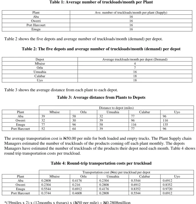
Coca Cola Company was our area of interest. Coca Cola Company has four major plants and five major depots in Nigeria. Considering a transportation problem faced by this company for six years. This problem involves the transportation of a truckload of their products from the four plants to the five depots at a minimal transportation cost. Production capacities of the Plants are adequate to satisfy their customers, but with limited available of number trucks. Table 1 shows the average number of truckloads/month per Plant.
Table 1: Average number of truckloads/month per Plant Plant Ave. number of truckloads/month per plant (Supply)
Aba 16
Owerri 16
Port Harcourt 16
Enugu 16
Table 2 shows the five depots and average number of truckloads/month (demand) per depot.
Table 2: The five depots and average number of truckloads/month (demand) per depot Depot Average truckloads/month per depot (Demand)
Mbaise 4
Orlu 7
Umuahia 16
Calabar 18
Uyo 18
Table 3 shows the average distance from each plant to each depot.
Table 3: Average distance from Plants to Depots Distance to depot (miles)
Plant Mbaise Orlu Umuahia Calabar Uyo
Aba 39 58 32 77 96
Owerri 32 30 39 96 116
Enugu 77 96 58 116 135
Port Harcourt 52 64 39 77 96
The average transportation cost is N50.00 per mile for both loaded and empty trucks. The Plant Supply chain Managers estimated the number of truckloads of the products coming off each plant monthly. The depots Managers have estimated the number of truckloads of the products their depot need each month. Table 4 shows round trip transportation costs per truckload.
Table 4: Round-trip transportation costs per truckload Transportation cost (Nm) per truckload per depot
Plant Mbaise Orlu Umuahia Calabar Uyo Aba 0.2808 0.4176 0.2304 0.5544 0.6912 Owerri 0.2304 0.216 0.2808 0.6912 0.8352 Enugu 0.5544 0.6912 0.4176 0.8352 0.9720 Port Harcourt 0.3744 0.4608 0.2808 0.5544 0.6912
www.theijes.com The IJES Page 5 Table 5 shows the four Costs element of transportation costs per truckload per plant of the company.
Table 5: Costs element of transportation costs per truckload per plant Cost Element of Transportation cost (Nm) per truckload per plant Plant Maintenance Fuel Personnel Loading/off loading
Aba 1.173 0.5867 0.2933 0.1467
Owerri 1.227 0.6133 0.3067 0.1533 Enugu 1.867 0.9333 0.4667 0.2333 Port Harcourt 1.280 0.6400 0.3200 0.1600
Table 6 shows the summary of the transportation problem
Table 6: Transporting costs, truckloads available and truckloads demanded Transportation cost (Nm) per truckload per depot
Plant Mbaise Orlu Umuahia Calabar Uyo Ave. available truckloads/plant Aba 0.2808 0.4176 0.2304 0.5544 0.6912 1152 Owerri 0.2304 0.2160 0.2808 0.6912 0.8352 1152 Enugu 0.5544 0.6912 0.4176 0.8352 0.9720 1152 Port Harcourt 0.3744 0.4608 0.2808 0.5544 0.6912 1152 Depot demand (truckloads) 288 504 1152 1296 1296
*(12months x 16 x 6years) = 1152truckloads (supply)
*(12months x 4 x 6years) = 288truckloads (demand)
As can be seen from table 4 and 5, there are some differences in transportation costs because of difference in the number of truckloads per depot and distances from plants to depots. This suggests that the realized sample may be considered acceptable representation of the transportation problem in Supply Chain Management.
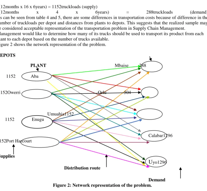
Management would like to determine how many of its trucks should be used to transport its product from each plant to each depot based on the number of trucks available.
Figure 2 shows the network representation of the problem. DEPOTS PLANT Mbaise 288 1152 Aba 1152Owerri Orlu 504 Umuahia1152 1152 Enugu Calabar1296 1152Port Harcourt Supplies
Uyo1296
Distribution route Demand Figure 2: Network representation of the problem.www.theijes.com The IJES Page 6
III.
ANALYSIS OF THE SURVEY DATA
The data obtained from the survey were analyzed using one approach Operation Research (OR). The OR approach involves the use of the tools of linear programming to model the problem.
The general problem of LP is the search for the optimal minimum of a linear function of variables constrained by linear relations (equations or inequalities).
Considering the company’spresent situation, the objective is to determine the number of truckload to be transported via each depot that provides the minimum total transportation cost. The cost for each truckload transported to each depot is given in table 4.
Solving this transportation problem with linear programming model, we use double-subscripted decision variables, with:
X11 = Number of truckload transportation from plant 1 (Aba Plant) to depot 1 (Mabise) X12 = Number of truckload transportation from plant 1 (Aba Plant) to depot 2 (Orlu) X13 = Number of truckload transportation from plant 1 (Aba Plant) to depot 3 (Umuahia) X14 = Number of truckload transportation from plant 1 (Aba Plant) to depot 4 (Calabar) X15 = Number of truckload transportation from plant 1 (Aba Plant) to depot 5 (Uyo) X21 = Number of truckload transportation from plant 2 (Owerri Plant) to depot 1 X22 = Number of truckload transportation from plant 2 (Owerri Plant) to depot 2 X23 = Number of truckload transportation from plant 2 (Owerri Plant) to depot 3 X24 = Number of truckload transportation from plant 2 (Owerri Plant) to depot 4 X25 = Number of truckload transportation from plant 2 (Owerri Plant) to depot 5 X31 = Number of truckload transportation from plant 3 (Enugu Plant) to depot 1 X32 = Number of truckload transportation from plant 3 (Enugu Plant) to depot 2 X33 = Number of truckload transportation from plant 3 (Enugu Plant) to depot 3 X34 = Number of truckload transportation from plant 3 (Enugu Plant) to depot 4 X35 = Number of truckload transportation from plant 3 (Enugu Plant) to depot 5 X41 = Number of truckload transportation from plant 4 (Port Harcourt Plant) to depot 1 X42 = Number of truckload transportation from plant 4 (Port Harcourt Plant) to depot 2 X43 = Number of truckload transportation from plant 4 (Port Harcourt Plant) to depot 3 X44 = Number of truckload transportation from plant 4 (Port Harcourt Plant) to depot 4 X45 = Number of truckload transportation from plant 4 (Port Harcourt Plant) to depot 5
3.1 GENERAL LP FORMATION FOR TRANSPORTATION PROBLEM The general transportation problem minimization model is:
Objective Function
Minimize Z = 𝑚𝑖=1 𝑛𝑗 =1𝐶𝑖𝑗𝑋𝑖𝑗 ………..……….... (1) Subject to:
1. Constraints on total available truckloads at each plant 𝑋𝑖𝑗
𝑛
𝑗 =1 = Si for i = 1, 2,…m ………...…….(2) 2. Constraints on total truckloads needed at each depot
𝑋𝑖𝑗 𝑚
𝑖=1 = Dj for j = 1, 2,….n. ………...(3) And Xij≤ 0 for all i and j.
j = 1, 2, 3 ….n; i = 1, 2… m Where
Z= objective function that minimized transportation costs (Nm) Xj = choice variable (truckloads) for which the problem solved
Cj = coefficient measuring the contribution of the jth choice variable to the objective function. Si and Dj = constraint or restrictions placed upon the problem.
The above problem can be solved using Software packages such as TORA and MS-Excel SOLVER, which provide following LP information: (Hamdy, 2008)
1. Information about the objective function: a. Objective function optimal value
www.theijes.com The IJES Page 7 b. Coefficient ranges (ranges of optimality). The range of optimality for each coefficient provides the range of values over which the current solution will remain optimal. Managers should focus on those objective coefficients that have a narrow range of optimality and coefficients near the endpoints of the range. 2. Information about the decision variables:
a. Their optimal values b. Their reduced costs
3. Information about the constraints: a. The amount of slack or surplus
b. The dual prices that represent the improvement in the value of the optimal solution per truck increase in the right-hand side.
c. Right-hand side ranges (ranges of feasibility) that represent the range over which the dual price is applicable. As the RHS increases, other constraints will become binding and limit the change in the value of the objective function.
Sensitivity Analysis Rules
For the objective function coefficients):
If 𝛿 𝐶𝑗/ΔCj≥ 1, the optimal solution will not change Where:
δCjis the actual increase (decrease) in the coefficient,
ΔCj is the minimum allowable increase (decrease) from the sensitivity analysis. For the RHS Constraints
If ∑δbj/Δbj ≥1, the optimal basis and number of truckloads monthly will not change δbjis the actual increase (decrease) in the coefficient,
Δbj is the minimum allowable increase (decrease) from the sensitivity analysis.
3.2 FORMULATION OF TRANSPORTATION PROBLEM AS A LINEAR PROGRAMMING MODEL The LP model and analysis exploit the structural advantages that accompany deterministic data and avoid representing potentially costly errors. In reality, the decisions occur sequentially over time. From the Survey data table 6:
The objective function can be represented as
Minimize Z = 0.2808X11 + 0.4176X12 + 0.2304X13 + 0.5544X14 + 0.6912X15 + 0.2304X21 + 0.2160X22 + 0.2808X23 + 0.6912X24 + 0.8352X25
+ 0.5544X31 + 0.6912X32 + 0.4176X33 + 0.8352X34 + 0.9720X35 ……….(4) + 0.3744X41 + 0.4608X42 + 0.2808X43 + 0.5544X44 + 0.6912X45{i.e. cost of transporting from coca cola plants to depots}
Subject to:
X11 + X12 + X13 + X14 + X15≤ 1080 Truckloads from Aba plant X21 + X22 + X23 + X24 + X25≤ 1080 Truckloads from Owerri plant X31 +X32 + X33 + X24 + X35≤ 1080 Truckloads from Enugu plant X41 + X42 + X43+ X44+ X45≤ 1080 Truckloads from Port Harcourt plant X11 + X21 + X31 + X41≥ 288 Truckloads to Mbaise depot
X12 + X22 + X32 + X42≥ 504 Truckloads to Orlu depot X13 +X23 + X33 + X43 ≥ 1152 Truckloads to Umuahia depot X14 + X24 + X34 + X44 ≥ 1296 Truckloads to Calabar depot X15 + X25 +X35 +X45≥ 1296 Truckloads to Uyo depot And X11, X12, ……X45all such values are ≥ 0
IV.
RESULTS AND DISCUSSIONS
The results of the data obtained are discussed, summarized and presented in simplex tableaus formats as well as in chart.
Solving the above transportation problem using TORA software package will result:
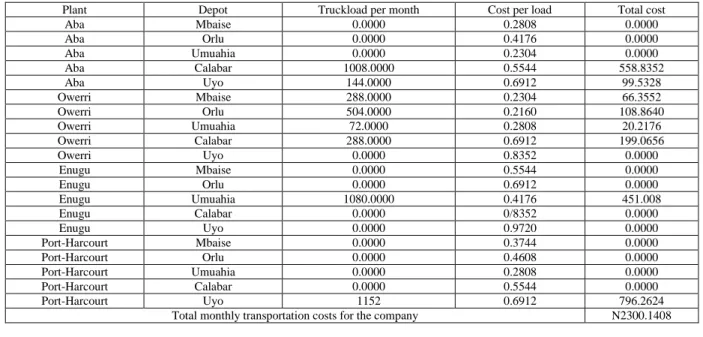
Minimum transportation cost Z = N2300.1408million. The amount (N2300.1408million) represents the minimum monthly transportation costs for the company to transport its products from the four plants to the five depots. From the computer result sheet, values in the Value column are assigning to our variables to determine the truck schedules for the company.
www.theijes.com The IJES Page 8 Table 7: Company truck schedule
Plant Depot Truckload per month Cost per load Total cost
Aba Mbaise 0.0000 0.2808 0.0000 Aba Orlu 0.0000 0.4176 0.0000 Aba Umuahia 0.0000 0.2304 0.0000 Aba Calabar 1008.0000 0.5544 558.8352 Aba Uyo 144.0000 0.6912 99.5328 Owerri Mbaise 288.0000 0.2304 66.3552 Owerri Orlu 504.0000 0.2160 108.8640 Owerri Umuahia 72.0000 0.2808 20.2176 Owerri Calabar 288.0000 0.6912 199.0656 Owerri Uyo 0.0000 0.8352 0.0000 Enugu Mbaise 0.0000 0.5544 0.0000 Enugu Orlu 0.0000 0.6912 0.0000 Enugu Umuahia 1080.0000 0.4176 451.008 Enugu Calabar 0.0000 0/8352 0.0000 Enugu Uyo 0.0000 0.9720 0.0000 Port-Harcourt Mbaise 0.0000 0.3744 0.0000 Port-Harcourt Orlu 0.0000 0.4608 0.0000 Port-Harcourt Umuahia 0.0000 0.2808 0.0000 Port-Harcourt Calabar 0.0000 0.5544 0.0000 Port-Harcourt Uyo 1152 0.6912 796.2624
Total monthly transportation costs for the company N2300.1408
From the computer result sheet, variable X11, which is Aba Plant to Mbaise Depot, the value – Number of truckloads per month is zero (see table 7), therefore, no truck movement from Aba Plant to Mbaise Depot. For variable X14, which is Aba Plant to Calabar Depot, the Value is 1008truckloads per month.
For X15, which Aba Plant to Uyo Depot the monthly number of truckloads is 144, and so on.
4.1 SENSITIVITY ANALYSIS SA OF THE INPUT DATA
In linear programming input data of the model can change within certain limits without causing the optimal solution to change. This is referred to as sensitivity analysis, (Taha 2008).
However, exactness of our LP model was confirmed by running sensitivity analysis. Through this the impact of uncertainty on the quality of the optimal solution was ascertained.
Through SA, it is possible to change the corresponding coefficient in the objective function and resolve the LP problem once more.These observations give rise to the investigation of the SA.
Knowing that the structure of the problem does not change, it is possible to investigate how changes in individual data elements change the optimal solution as follows:
• If nothing else changes except the objective function value when slightly change, the number of truckloads, transportation cost and the nature of the solution changes considerably.
• On the other hand, if the transportation cost is kept fixed, and the number of truckloads needed increase or drop by e.g. 10% and there would be no major impact on the solution, Firm would still transport their products and take the initial LP problem solution into consideration.
This result shows that maintenance, fuel, driver’s welfare, mileage, and loading/offloading costs have significant effect on transportation costs. Given these constrains due consideration, transportation costs will be minimize. Figure 3 represents the four costs element of transportation cost/month per plant for six years.
This shows that 39.20% of the Company total expenditure under transportation sector for six years was on maintenance alone. While 20.79%, 8.79% and 5.05% was on fuel, driver’s welfare and loading/offloading respectively.
www.theijes.com The IJES Page 9 Figure 3: The four costs element of transportation cost/month per plant for six years
The solution recommends the reduction in cost of maintenance per truck. The results conclude that the optimal decision is not to increase the number of truckloads per depot, but to reduce the cost of maintenance of trucks by adopting predictive and preventive maintenance rather than corrective maintenance. It also recommends that the issue of conventional wisdom (i.e. if it is not broke, then don’t fix it or that parts are expendable to some degree) should be eliminated.
V.
CONCLUSION
Managing data when constructing LP models can be challenging. The data used in LP models is often clouded with uncertainty. A transportation problem was developed with respect to the operations of the Coca Cola Company of Aba, Owerri, Port Harcourt and Enugu in its depots in Mbaise, Orlu, Umuahia, Calabar and Uyo with respect to truckload movement between the cities. The data obtained in the study was used with respect to the cities, an objective equation developed took this from: Z = 0.2808X11 + ……. + 0.6912X45 (ie cost of transportation from Coca Cola plants to depots). The problem was solved by using TORA software package. The objective was determined, deduced, solved, and the minimum cost for the operation obtained. An industrial case was used to demonstrate the feasibility of applying the LP method to real-world transportation costs problem. Consequently, the LP and SA methods developed in this work yield an efficient compromise solution and overall decision maker satisfaction.
REFERENCE
[1] Arntzen B.C, Brown G.G, Harrison T.P and Trafton L.L (1995), “Global supply chain management at Digital Equipment
Corporation”, Interfaces, vol.25, pp. 69-93
[2] Dantzig, G.B. and Thapa, M.N. (1997). Linear programming 1: Introduction. Springer-Verlag. [3] Dantzig, G.B., (1963) Linear Programming and Extensions, PrincetonUniversity Press.
[4] Geunes J.B, and Chang, B., (2002) Operations Research models for Supply Chain Management and Design, Working paper, University of Florida, Forthcoming in C.A. Floudas and P.M. Pardalos, editors, Encyclopedia of Optimization, Kluwer Academic Publishers, Dordrecht, The Netherlands.
[5] Hamdy A. Taha (2008), Operations Research, An Introduction eight edition, Prentice – Hall, Inc. Upper Saddle River, New JerseyU.S.A.
[6] Ganeshan, R. and Terry P.H., (1995), An Introduction to Supply Chain ManagementInterfaces, vol.1, pp. 2-3
[7] Tayur, S., Ganeshan, R. and Magazine M. (eds.), (1999) Quantitative models for supply chain management, 2nd ed., Kluwer Academic Publishers, Boston.
0 0.2 0.4 0.6 0.8 1 1.2 1.4 1.6 1.8 2 1 2 3 4 C OS T PLANT
FOUR COSTS ELEMENT OF TRANSPORTATION COST
Maintenance Fuel Personnel Loading/Off loading