University of Nebraska - Lincoln
DigitalCommons@University of Nebraska - Lincoln
CSE Conference and Workshop Papers
Computer Science and Engineering, Department of
11-10-2012
HOG: Distributed Hadoop MapReduce on the
Grid
Chen He
University of Nebraska-Lincoln, [email protected]
Derek J. Weitzel
University of Nebraska-Lincoln, [email protected]
David Swanson
University of Nebraska-Lincoln, [email protected]
Ying Lu
University of Nebraska-Lincoln, [email protected]
Follow this and additional works at:
http://digitalcommons.unl.edu/cseconfwork
Part of the
OS and Networks Commons
, and the
Systems Architecture Commons
This Article is brought to you for free and open access by the Computer Science and Engineering, Department of at DigitalCommons@University of Nebraska - Lincoln. It has been accepted for inclusion in CSE Conference and Workshop Papers by an authorized administrator of
DigitalCommons@University of Nebraska - Lincoln.
He, Chen; Weitzel, Derek J.; Swanson, David; and Lu, Ying, "HOG: Distributed Hadoop MapReduce on the Grid" (2012).CSE
Conference and Workshop Papers. 231.
HOG: Distributed Hadoop MapReduce on the Grid
Chen He, Derek Weitzel, David Swanson, Ying Lu
Computer Science and Engineering University of Nebraska – Lincoln
Email:{che, dweitzel, dswanson, ylu}@cse.unl.edu
Abstract—MapReduce is a powerful data processing platform for commercial and academic applications. In this paper, we build a novel Hadoop MapReduce framework executed on the Open Science Grid which spans multiple institutions across the United States – Hadoop On the Grid (HOG). It is different from previous MapReduce platforms that run on dedicated environments like clusters or clouds. HOG provides a free, elastic, and dynamic MapReduce environment on the opportunistic resources of the grid. In HOG, we improve Hadoop’s fault tolerance for wide area data analysis by mapping data centers across the U.S. to virtual racks and creating multi-institution failure domains. Our modifications to the Hadoop framework are transparent to existing Hadoop MapReduce applications. In the evaluation, we successfully extend HOG to 1100 nodes on the grid. Additionally, we evaluate HOG with a simulated Facebook Hadoop MapReduce workload. We conclude that HOG’s rapid scalability can provide comparable performance to a dedicated Hadoop cluster.
Keywords- MapReduce, Grid computing, Middleware
I. INTRODUCTION
MapReduce [1] is a framework pioneered by Google for processing large amounts of data in a distributed environment. Hadoop [2] is the open source implementation of the MapRe-duce framework. Due to the simplicity of its programming model and the run-time tolerance for node failures, MapRe-duce is widely used by companies such as Facebook [3], the New York Times [4], etc. Futhermore, scientists also employ Hadoop to acquire scalable and reliable analysis and storage services. The University of Nebraska-Lincoln constructed a 1.6PB Hadoop Distributed File System to store Compact Muon Solenoid data from the Large Hadron Collider [5], as well as data for the Open Science Grid (OSG) [6]. In the University of Maryland, researchers developed blastreduce based on Hadoop MapReduce to analyze DNA sequences [7]. As Hadoop MapReduce became popular, the number and scale of MapReduce programs became increasingly large.
To utilize Hadoop MapReduce, users need a Hadoop plat-form which runs on a dedicated environment like a cluster or cloud. In this paper, we construct a novel Hadoop platform, Hadoop on the Grid (HOG), based on the OSG [6] which can provide scalable and free of charge services for users who plan to use Hadoop MapReduce. It can be transplanted to other large scale distributed grid systems with minor modifications. The OSG, which is the HOG’s physical environment, is composed of approximately 60,000 CPU cores and spans 109 sites in the United States. In this nation-wide distributed system, node failure is a common occurrence [8]. When running on the OSG, users from institutions that do not own
resources run opportunistically and can be preempted at any time. A preemption on the remote OSG site can be caused by the processing job running over allocated time, or if the owner of the machine has a need for the resources. Preemption is determined by the remote site’s policies which are outside the control of the OSG user. Therefore, high node failure rate is the largest barrier that HOG addresses.
Hadoop’s fault tolerance focuses on two failure levels and uses replication to avoid data loss. The first level is the node level which means a node failure should not affect the data integrity of the cluster. The second level is the rack level which means the data is safe if a whole rack of nodes fail. In HOG, we introduce another level which is the site failure level. Since HOG runs on multiple sites within the OSG. It is possible that a whole site could fail. HOG’s data placement and replication policy takes the site failure into account when it places data blocks. The extension to a third failure level will also bring data locality benefits which we will explain in Section III.
The rest of this paper is organized as follows. Section II gives the background information about Hadoop and the OSG. We describe the architecture of HOG in section III. In section IV, we show our evaluation of HOG with a well-known workload. Section V briefly describes related work, and VI discusses possible future research. Finally, we summarize our conclusions in Section VII.
II. BACKGROUND
A. Hadoop
A Hadoop cluster is composed of two parts: Hadoop Dis-tributed File System and MapReduce.
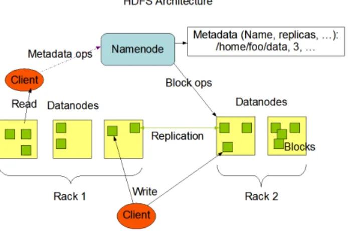
A Hadoop cluster uses Hadoop Distributed File System (HDFS) [9] to manage its data. HDFS provides storage for the MapReduce job’s input and output data. It is designed as a highly fault-tolerant, high throughput, and high capacity distributed file system. It is suitable for storing terabytes or petabytes of data on clusters and has flexible hardware require-ments, which are typically comprised of commodity hardware like personal computers. The significant differences between HDFS and other distributed file systems are: HDFS’s write-once-read-many and streaming access models that make HDFS efficient in distributing and processing data, reliably storing large amounts of data, and robustly incorporating heteroge-neous hardware and operating system environments. It divides each file into small fixed-size blocks (e.g., 64 MB) and stores multiple (default is three) copies of each block on cluster node disks. The distribution of data blocks increases throughput and 2012 SC Companion: High Performance Computing, Networking Storage and Analysis
Fig. 1. HDFS Structure. Source: http://hadoop.apache.org
fault tolerance. HDFS follows the master/slave architecture. The master node is called the Namenode which manages the file system namespace and regulates client accesses to the data. There are a number of worker nodes, called Datanodes, which store actual data in units of blocks. The Namenode maintains a mapping table which maps data blocks to Datanodes in order to process write and read requests from HDFS clients. It is also in charge of file system namespace operations such as closing, renaming, and opening files and directories. HDFS allows a secondary Namenode to periodically save a copy of the metadata stored on the Namenode in case of Namenode failure. The Datanode stores the data blocks in its local disk and executes instructions like data replacement, creation, deletion, and replication from the Namenode. Figure 1 (adopted from Apache Hadoop Project [10]) illustrates the HDFS architecture.
A Datanode periodically reports its status through a heart-beat message and asks the Namenode for instructions. Every Datanode listens to the network so that other Datanodes and users can request read and write operations. The heartbeat can also help the Namenode to detect connectivity with its Datanode. If the Namenode does not receive a heartbeat from a Datanode in the configured period of time, it marks the node down. Data blocks stored on this node will be considered lost and the Namenode will automatically replicate those blocks of this lost node onto some other datanodes.
Hadoop MapReduce is the computation framework built upon HDFS. There are two versions of Hadoop MapReduce: MapReduce 1.0 and MapReduce 2.0 (Yarn [11]). In this paper, we only introduce MapReduce 1.0 which is comprised of two stages: map and reduce. These two stages take a set of input key/value pairs and produce a set of output key/value pairs. When a MapReduce job is submitted to the cluster, it is divided into M map tasks and R reduce tasks, where each map task will process one block (e.g., 64 MB) of input data.
A Hadoop cluster uses slave (worker) nodes to execute map and reduce tasks. There are limitations on the number of map and reduce tasks that a worker node can accept and execute
simultaneously. That is, each worker node has a fixed number of map slots and reduce slots. Periodically, a worker node sends a heartbeat signal to the master node. Upon receiving a heartbeat from a worker node that has empty map/reduce slots, the master node invokes the MapReduce scheduler to assign tasks to the worker node. A worker node who is assigned a map task reads the content of the corresponding input data block from HDFS, possibly from a remote worker node. The worker node parses input key/value pairs out of the block, and passes each pair to the user-defined map function. The map function generates intermediate key/value pairs, which are buffered in memory, and periodically written to the local disk and divided into R regions by the partitioning function. The locations of these intermediate data are passed back to the master node, which is responsible for forwarding these locations to reduce tasks.
A reduce task uses remote procedure calls to read the intermediate data generated by the M map tasks of the job. Each reduce task is responsible for a region (partition) of intermediate data with certain keys. Thus, it has to retrieve its partition of data from all worker nodes that have executed the M map tasks. This process is called shuffle, which involves many-to-many communications among worker nodes. The reduce task then reads in the intermediate data and invokes the reduce function to produce the final output data (i.e., output key/value pairs) for its reduce partition.
B. Open Science Grid
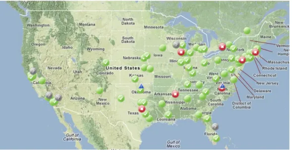
The OSG [6] is a national organization that provides ser-vices and software to form a distributed network of clusters. OSG is composed of 100+ sites primarily in the United States. Figure 2 shows the OSG sites across the United States.
Each OSG user has a personal certificate that is trusted by a Virtual Organization (VO) [12]. A VO is a set of individuals and/or institutions that perform computational research and share resources. A User receives a X.509 user certificate [13] which is used to authenticate with remote resources from the VO.
Users submit jobs to remote gatekeepers. OSG gatekeepers are a combination of different software based on the Globus Toolkit [14], [15]. Users can use different tools that can communicate using the Globus resource specification language [16]. The common tool is Condor [17]. Once Jobs arrive at the gatekeeper, the gatekeeper will submit them to the remote batch scheduler belonging to the sites. The remote batch scheduler will launch those jobs according to its scheduling policy.
Sites can provide storage resources accessible with the user’s certificate. All storage resources are again accessed by a set of common protocols, Storage Resource Manager (SRM) [18] and Globus GridFTP [19]. SRM provides an interface for metadata operations and refers transfer requests to a set of load balanced GridFTP servers. The underlying storage technologies at the sites are transparent to users. The storage is optimized for high bandwidth transfers between sites, and high throughput data distribution inside the local site.
Fig. 2. OSG sites across the United States. Source: http://display.grid.iu.edu/
III. ARCHITECTURE
The architecture of HOG is comprised of three components. The first is the grid submission and execution component. In this part, the Hadoop worker nodes requests are sent out to the grid and their execution is managed. The second major com-ponent is the Hadoop distributed file system (HDFS) that runs across the grid. And the third component is the MapReduce framework that executes the MapReduce applications across the grid.
A. Grid Submission and Execution
Grid submission and execution is managed by Condor and GlideinWMS, which are generic frameworks designed for resource allocation and management. Condor is used to manage the submission and execution of the Hadoop worker nodes. GlideinWMS is used to allocate nodes on remote sites transparently to the user.
When the HOG starts, a user can request Hadoop worker nodes to run on the grid. The number of nodes can grow and shrink elastically by submitting and removing the worker node jobs. The Hadoop worker node includes both the datanode and the tasktracker processes. The Condor submission file is shown in Listing 1. The submission file specifies attributes of the jobs that will run the Hadoop worker nodes.
The requirements line enforces a policy that the Hadoop worker nodes should only run at these sites. We restricted our experiments only to these sites because they provide publicly reachable IP addresses on the worker nodes. Hadoop worker nodes must be able to communicate to each other directly for data transferring and messaging. Thus, we restricted execution to 5 sites. FNAL_FERMIGRID and
USCMS-FNAL-WC1 are clusters at Fermi National Acceler-ator LaborAcceler-atory. UCSDT2 is the US CMS Tier 2 hosted at the University of California – San Diego. AGLT2is the US Atlas Great Lakes Tier 2 hosted at the University of Michigan.
Listing 1. Condor Submission file for HOG
universe = vanilla
requirements = GLIDEIN_ResourceName =?= " FNAL_FERMIGRID" || GLIDEIN_ResourceName =?= "USCMS-FNAL-WC1" || GLIDEIN_ResourceName =?=
"UCSDT2" || GLIDEIN_ResourceName =?= " AGLT2" || GLIDEIN_ResourceName =?= "MIT_CMS" executable = wrapper.sh output = condor_out/out.$(CLUSTER).$(PROCESS) error = condor_out/err.$(CLUSTER).$(PROCESS) log = hadoop-grid.log should_transfer_files = YES when_to_transfer_output = ON_EXIT_OR_EVICT OnExitRemove = FALSE PeriodicHold = false x509userproxy = /tmp/x509up_u1384 queue 1000
MIT_CMSis the US CMS Tier 2 hosted at the Massachusetts Institute of Technology.
The executable specified in the condor submit file is a simple shell wrapper script that will initialize the Hadoop worker node environment. The wrapper script follows these steps in order to start the Hadoop worker node:
1) Initialize the OSG operating environment 2) Download the Hadoop worker node executables 3) Extract the worker node executables and set late binding
configurations
4) Start the Hadoop daemons
5) When the daemons shut down, clean up the working directory.
Initializing the OSG operating environment sets the required environment variables for proper operation on an OSG worker node. For example, it can set the binary search path to include grid file transfer tools that may be installed in non-standard locations.
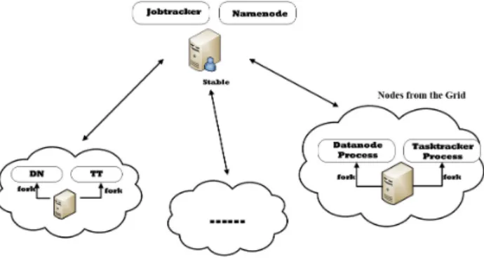
Fig. 3. HOG Architecture
In the evaluation the Hadoop executables package was compressed to 75MB, which is small enough to transfer to worker nodes. This package includes the configuration file, the deployment scripts, and the Hadoop jars. It can be downloaded from a central repository hosted on a web server. Decompression of the package takes a trivial amount of time on the worker nodes, and is not considered in the evaluation. The wrapper must set configuration options for the Hadoop worker nodes at runtime since the environment is not known until it reaches the node where it will be executing. The Hadoop configuration must be dynamically changed to point the value of mapred.local.dir to a worker node local directory. If the Hadoop working directory is on shared stor-age, such as a network file system, it will slow computation due to file access time and we will lose data locality on the worker nodes. We avoid using shared storage by utilizing GlideinWMS’s mechanisms for starting a job in a worker node’s local directory.
B. Hadoop On The Grid
The Hadoop instance that is running on the grid has two major components, Hadoop Distributed File System (HDFS) and MapReduce, shown in Figure 3. The master servers, Namenode for HDFS and JobTracker for MapReduce, are single points of failure for the HOG system, therefore they reside on a stable central server. If the master server becomes unavailable, execution of MapReduce jobs will stop and the HDFS file system will become unavailable (though no data will be lost). When the grid jobs start, the slave servers will report to the single master server.
Hadoop requires worker nodes to be reachable by each other. Some clusters in the Open Science Grid are designed to be behind one or more machines that provide Network Address Translation (NAT) access to the Internet. Hadoop is unable to talk to nodes behind a remote NAT because NAT blocks direct access. Therefore, we are limited to sites in the OSG that have a public IPs on their worker nodes.
Failures on the grid are very common due to the site un-availability and preemption. It is important that HOG responds quickly to recover lost nodes by redistributing data and pro-cessing to remaining nodes, and requesting more nodes from the grid. The Hadoop master node receives heartbeat messages
from the worker nodes periodically reporting their health. In HOG, we decreased the time between heartbeat messages and decreased the timeout time for the worker nodes. If the worker nodes do not report every 30 seconds, then the node is marked dead for both the namenode and jobtracker. The traditional value for theheartbeat.recheck.interval
is 15 minutes for a node before declaring the node dead. 1) HDFS On The Grid: Creating and maintaining a dis-tributed filesystem on a disparate set of resources can be challenging. Hadoop is suited for this challenge as it is designed for frequent failures.
In traditional Hadoop, the datanode will contact the namenode and report its status including information on the size of the disk on the remote node and how much is available for Hadoop to store. The namenode will determine what data files should be stored on the node by the location of the node using rack awareness and by the percent of the space that is used by Hadoop.
Rack awareness provides both load balancing and improved fault tolerance for the file system. Rack awareness is designed to separate nodes into physical failure domains and to load balance. It assumes that bandwidth inside a rack is much larger than the bandwidth between racks, therefore the namenode will use the rack awareness to place data closer to the source. For fault tolerance, the namenode uses rack awareness to put data on the source rack and one other rack to guard against whole rack failure. An entire rack could fail if a network component fails, or if power is interrupted to the rack power supply unit. However, rack awareness requires knowledge of the physical layout of the cluster. On the grid, users are unlikely to have knowledge of the physical layout of the cluster, therefore traditional rack awareness would be impractical. Instead, rack awareness in HOG is extended to site awareness. We differentiate nodes based on their sites.
Sites are common failure domains, therefore fitting well into the existing rack awareness model. Sites in the OSG are usually one or a few clusters in the same administrative domain. There can be many failures that can cause an entire site to go down, such as a core network component failure, or a large power outage. These are the errors that rack awareness was designed to mitigate.
Also, sites usually have very high bandwidth between their worker nodes, and lower bandwidth to the outside world. This is synonymous with HDFS’s assumptions about the rack, that the bandwidth inside the rack is much larger than the bandwidth between racks.
Sites are detected and separated by the reported host-names of the worker nodes. Since the worker nodes need to be publicly addressable, they will likely have DNS names. For example, the DNS names will be broken up into workername.site.edu. The worker nodes will be separated depending on the last two groups, thesite.edu. All worker nodes with the same last two groups will be determined to be in the same site.
The detection and separation is done by a site aware-ness script, defined in the Hadoop configuration as
topology.script.file.name. It is executed each time a new node is discovered by the namenode and the jobtracker. In addition to site-awareness, we increased the default replication factor for all files in HDFS to 10 replicas from the traditional replication factor for Hadoop of 3. Simultaneous preemptions on a site is common in the OSG since higher priority users may submit many jobs, preempting many of our HDFS instances. In order to address simultaneous preemp-tions, both site awareness and increased replication are used. Also, increased replication will guard against preemptions occurring faster than the namenode can replicate missing data blocks. Too many replicas would impose extra replication overhead for the namenode. Too few would cause frequent data failures in the dynamic HOG environment. 10 replicas was the experimental number which worked for our evaluation.
2) MapReduce On The Grid: The goal of our implementa-tion is to provide a Hadoop platform comparable to that of a dedicated cluster for users to run on the grid. They should not have to change their MapReduce code in order to run on our adaptation of Hadoop. Therefore, we made no API changes to MapReduce, only underlying changes in order to better fit the grid usage model.
When the grid job begins, it starts the tasktracker on the remote worker node. The tasktracker is in charge of managing the execution of Map and Reduce tasks on the worker node. When it begins, it contacts the jobtracker on the central server which marks the node available for processing.
The tasktrackers report their status to the jobtracker and accept task assignments from it. In the current version of HOG, we follow Apache Hadoop’s FIFO job scheduling policy with speculative execution enabled. At any time, a task has at most two copies of execution in the system.
The communication between the tasktracker and the job-tracker is based on HTTP. In the HOG system, the HTTP requests and responses are over the WAN which has high latency and long transmission time compared with the LAN of a cluster. Because of this increased communication latency, it is expected that the startup and data transfer initiations will be increased.
Just as site awareness affects data placement, it also affects the placement of Map jobs for processing. The default Hadoop scheduler will attempt to schedule Map tasks on nodes that have the input data. If it is unable to find a data local node, it will attempt to schedule the Map task in the same site as the input data. Again, Hadoop assumes the bandwidth inside a site is greater than the bandwidth between sites.
IV. EVALUATION
A. Experimental Setup
In this section, we employ a workload from the Facebook production cluster to verify HOG performance and reliability. The Facebook workload is used to construct the performance baseline between our HOG and the dedicated Hadoop cluster. We create a submission schedule that is similar to the one used by Zaharia et al. [3]. They generated a submission schedule for 100 jobs by sampling job inter-arrival times and input sizes
from the distribution seen at Facebook over a week in October 2009. By sampling job inter-arrival times at random from the Facebook trace, they found that the distribution of inter-arrival times was roughly exponential with a mean of 14 seconds.
They also generated job input sizes based on the Facebook workload, by looking at the distribution of number of map tasks per job at Facebook and creating datasets with the correct sizes (because there is one map task per 64 MB input block). Job sizes were quantized into nine bins, listed in Table I, to make it possible to compare jobs in the same bin within and across experiments. Our submission schedule has similar job sizes and job inter-arrival times. In particular, our job size distribution follows the first six bins of job sizes shown in Table I, which cover about 89% of the jobs at the Facebook production cluster. Because most jobs at Facebook are small and our test cluster is limited in size, we exclude those jobs with more than 300 map tasks. Like the schedule in [3], [20], the distribution of inter-arrival times is exponential with a mean of 14 seconds, making our total submission schedule 21 minutes long.
TABLE I
FACEBOOKPRODUCTIONWORKLOAD
%Jobs #Maps # of jobs Bin #Maps at Facebook in Benchmark in Benchmark
1 1 39% 1 38 2 2 16% 2 16 3 3-20 14% 10 14 4 21-60 9% 50 8 5 61-150 6% 100 6 6 151-300 6% 200 6 7 301-500 4% 400 4 8 501-1500 4% 800 4 9 >1501 3% 4800 4
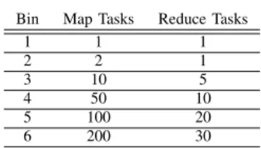
However, the authors [3] only provide the number of map tasks required by each job. In this paper, we introduce reduce tasks to the workload. They number in a non-decreasing pattern compared to job’s map tasks. They are listed in Table II.
TABLE II
TRUNCATED WORKLOAD FOR THIS PAPER
Bin Map Tasks Reduce Tasks
1 1 1 2 2 1 3 10 5 4 50 10 5 100 20 6 200 30
In this paper, we define the term “equivalent performance”. Two systems have equivalent performance if they have the same response time for a given workload. We will build the HOG system and a Hadoop cluster to achieve equivalent performance. Because the size of a Hadoop cluster is fixed, we need to tune the number of nodes in the HOG system to achieve equivalent performance.
In order to avoid the interference caused by growing and shrinking in HOG, we first configure a given number of
TABLE III
DEDICATEDMAPREDUCECLUSTERCONFIGURATION
Nodes Quantity Hardware and Hadoop Configuration Master node 1 2 single-core 2.2GHz
Opteron-248 CPUs, 8GB RAM, 1Gbps Ethernet Slave nodes-I 20 2 dual-core
2.2GHz Opteron-275 CPUs, 4GB RAM, 1 Gbps Ethernet, 4 map and 1 reduce slots per node Slave nodes-II 10 2 single-core
2.2GHz Optron-64 CPUs, 4GB RAM, 1 Gbps Ethernet, 2 map and 1 reduce slots per node
nodes that HOG will achieve and wait until HOG reaches this number. Then, we start to upload input data and execute the evaluation workload.
We first built a Hadoop cluster which contains 30 worker nodes that are configured as one rack. The worker nodes-I group contains 20 nodes. Each of them has 2 dual-core CPUs. The worker nodes-II group contains 10 nodes, each with only 2 single-core CPUs. The cluster is composed of 100 CPUs. Detailed hardware information is listed in the Table III. Our Hadoop cluster is based on Hadoop 0.20. We used loadgen, which is a test example in Hadoop source code and used in evaluating Hadoop schedulers [3], [20] to get the performance baseline. We configure 1 reduce slot for each worker node because there is only one Ethernet card in each node and the reduce stage involves intensive network data transfer. Also, configure 1 map slot per core. Other configuration parameters follow the default settings of Hadoop from Apache [9]. For the HOG configuration, we configure each node to have 1 map slot and 1 reduce slot, since the job is allocated 1 core on the remote worker node.
50 100 250 500 1000 1500 2000 2500 3000 3500 4000 4500 5000 40 50 55 60 99 100 132 160 171 180 974 1101
HOG vs. Cluster Equivalent Performance
Number of Nodes in HOG
Response Time (second)
HOG Cluster (100 cores)
Logrithmic
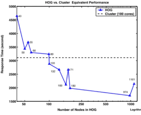
Fig. 4. HOG System Performance
B. Equivalent Performance
In the Figure 4, the dashed line is the response time of the workload in our local cluster and the solid line is the response time of the HOG cluster executing on the OSG. We can see the solid line crosses the dashed line when the HOG has 99 to 100 nodes. We see that the HOG system needs [99,100]
nodes to achieve equivalent performance when compared to our 100-core Hadoop cluster.
We performed 3 runs at each sampling point. The sampling point was set as the maximum number of nodes configured to join HOG. We waited until the available nodes reached the maximum and started execution. During execution, nodes left the system, and other nodes replaced them, but we only marked on the graph with the maximum nodes that could be available.
We can also see from Figure 4 that the response time of the workload does not always decrease with the increasing number of nodes in the HOG system. There are many reasons. As is well known, HOG is based on a dynamic environment and the worker nodes are opportunistic. Once some nodes leave, the HOG system will automatically request more nodes from the OSG to compensate for the missing worker nodes. However, it takes time for requesting, configuring, and starting a new worker node. At the same time, the newly added nodes have no data. HOG has to either copy data to those nodes or start tasks without data locality. The more dynamic the resource environment is, the longer the response time will be.
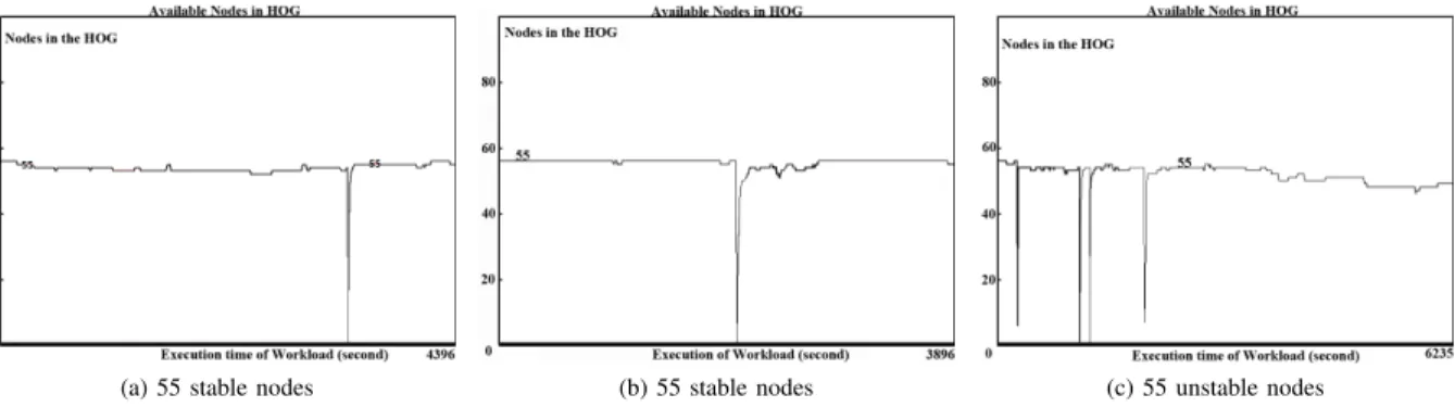
In order to verify our analysis, we examine three executions of the HOG system with 55 nodes. Figure 5 shows the number of available nodes in the HOG system during the workload execution. We set the maximum number of nodes in HOG to 55, though the reported number of nodes in the figure fluctuated above 55 momentarily as nodes left but where not reported dead for their heartbeat timeout. Figure 5a and 5b show smaller node change compared with Figure 5c. In Table IV, we can see Figure 5b shows the shortest response time and Figure 5c shows the longest response time. We also use the area which is beneath the curve during the execution of the workload, to demonstrate the node fluctuation. It also verified our analysis of the workload executions.
We can avoid this fluctuation by running multiple copies of MapReduce jobs in the HOG system. Currently, Hadoop only uses multiple executions for slower tasks (1/3 slower than average) execution, and at most two copies for a task. In our future work, we will make all tasks have configurable number of copies running in the HOG and take the fastest as the result. In this way, the HOG can finish MapReduce jobs faster even when there are some nodes missing.
C. Scalability
As we mentioned in our introduction, HOG is scalable. If users want to increase the number of nodes in the HOG, they can submit more Condor jobs for extra nodes. They can use the HDFS balancer to balance the data distribution. In our ex-periments, we elastically extend our system from 132 to 1101 nodes and run the workload to verify HOG’s performance. Figure 4 shows the response time of the workload in different number of nodes in HOG. In general, we can obtain shorter response time if there are more nodes in the HOG system.
However, there are downsides if we keep increasing the size of HOG. First of all, the data movement and replication cannot be neglected because this process will impose extra overhead
(a) 55 stable nodes (b) 55 stable nodes (c) 55 unstable nodes Fig. 5. HOG Node Fluctuation
TABLE IV AREA BENEATH CURVES
Figure No. Response Time Area 5a 4396 181020 5b 3896 172360 5c 6235 252455
on the Namenode and Datanode. The performance of HOG will degrade if replication happens during the execution of a workload.
Secondly, the probability of losing a node rises with the increasing of cores in HOG. As we can see in the Table IV, the more node fluctuation, the longer response we will get for a given workload. The performance may degrade as node failure increases.
D. Experiences
We learned some lessons during the construction of HOG. We list them in this section.
1) Abandoned Data Nodes: In our first iteration of HOG, the Hadoop daemons were started with the Hadoop-provided startup scripts. These scripts perform a “double fork”, where the daemons will leave the process tree of the script and run independently in their own process tree. Unfortunately, many site resource managers are unable to preempt a daemon that has double forked, since they only look at the process tree of the initial executable.
When a site wishes to preempt a HOG node, it will first kill the process tree, then remove the job’s working directories. Since HOG daemons were outside of the process tree, they continued after the site killed the grid job. When the site deleted the job’s working directories, the datanode would fail, but the tasktracker would continue working. When the tasktracker accepted a map or reduce job, it would fail immediately as it was unable to save the input data to disk.
In order to solve the abandoned daemon problem, we implemented two fixes. First, we modified the Hadoop source code to enable it to periodically check the working directory for writability and readability by writing a small file and reading it back. We modified the Datanode.java class in Hadoop. The original implementation ofDatanode.javachecks
the disk availability when it starts. We add the disk availability check in service code and do the check every 3 minutes. If these tests fail, then the daemons will shut themselves down. Second, we changed how we started the daemons to keep them in the same process tree. In this implementation, the datanode and task tracker would not be lost to the system as it was a direct child process of the wrapper script.
2) Disk Overflow: During our experiments, we noticed many failures during the execution of a MapReduce sample workflow. The errors indicated that the worker nodes were running out of disk. Our replication factor and the high latency between some nodes on the grid caused the disk overflows. It is also worth noting that Hadoop will not delete map intermediate data until the entire job is done.
The high replication factor for HOG allows for very good data locality. With the data on the same node as the map execution, reading in the data is very quick. But, each reduce needs to get data from each mapper. Since the reduce stages run on other sites, the data will need to be transferred over the WAN, which will be much more slowly than the map tasks. As map tasks complete, the map tasks for subsequent jobs are executed. Meanwhile, reduce tasks are completing much slower. This leads to a buildup of intermediate map output on the worker nodes, causing the nodes to fail due to lack of disk space. These failures are reported to the jobtracker as a worker nodes out of disk error.
V. RELATEDWORK
Our platform is different from running Hadoop On Demand (HOD) [21] on the Grid. HOD will create a temporary Hadoop platform on the nodes obtained from the Grid Scheduler and shut down Hadoop after the MapReduce job finishes. For frequent MapReduce requests, HOD has high reconstruction overhead, fixed node number, and a randomly chosen head node. Compared to HOD, HOG does not have reconstruction time, has a scalable size, and has a static dedicated head node which hosts the JobTracker and the Namenode. Though HOG does lose nodes, and has to rebalance data frequently, HOD reconstructs the entire Hadoop cluster while HOG only redistributes data from nodes that are lost by preemption.
MOON [22] creates a MapReduce framework on oppor-tunistic resources. However, they require dedicated nodes to
provide an anchor to supplement the opportunistic resources. Additionally, the scalability of MOON is limited by the size of the dedicated anchor cluster. HOG stores all data in the grid resources and uses replication schemes to guarantee data availability while MOON requires one replica of each data block stored on the anchor cluster. The stable central server in HOG does resemble an anchor, but the scalability of HDFS is not limited by the size of disk on the central server, rather on the disk on the many nodes on the grid.
VI. FUTUREWORK
In this paper, we proved the feasibility of deploying HOG, which can achieve equivalent performance with a dedicated cluster. However, there are still many issues we need to resolve.
Security of Hadoop is a very important issue for HOG. In our current version, HOG uses plain HTTP to achieve the RPC between nodes. In the OSG, users have to use an authorized certificate to access resources. To avoid a man in the middle attack, we will introduce PKI [23] to encrypt the HTTP communication of HOG because Kerberos [24] used by Hadoop is not well supported by the OSG.
To shrink and grow HOG, we need to consider how the data blocks will be moved and replicated. We can use the rate of shrinking and growing to detect the instability of HOG to set the number of replicas of the files and the number of redundant MapReduce tasks. [25]
VII. CONCLUSION
In this paper, we created a Hadoop infrastructure based on the Open Science Grid. Our contribution includes the detection and resolution of the zombie datanode problem, site-awareness, and a data availability solution for HOG. Through the evaluation, we found that the unreliability of the grid makes Hadoop on the grid challenging. The HOG system uses the Open Science Grid, and is therefore free for researchers. We found that the HOG system, though difficult to develop, can reliably achieve equivalent performance with a dedicated cluster. Additionally, we showed that HOG can scale to 1101 nodes with potential scalability at larger numbers. We will work on security and enabling multiple copies of map and reduce tasks execution in the future.
ACKNOWLEDGMENT
This research was done using resources provided by the Open Science Grid, which is supported by the National Science Foundation and the U.S. Department of Energy’s Office of Science. This work was completed utilizing the Holland Computing Center of the University of Nebraska. The authors acknowledge support from NSF awards #1148698 and #1018467.
REFERENCES
[1] J. Dean and S. Ghemawat, “Mapreduce: simplified data processing on large clusters,” inProceedings of the 6th conference on Symposium on Opearting Systems Design & Implementation - Volume 6, ser. OSDI’04. Berkeley, CA, USA: USENIX Association, 2004, pp. 10–10.
[2] A. Bialecki, M. Cafarella, D. Cutting, and O. OMALLEY, “Hadoop: a framework for running applications on large clusters built of commodity hardware,”Wiki at http://lucene.apache.org/hadoop, vol. 11, 2005. [3] M. Zaharia, D. Borthakur, J. Sen Sarma, K. Elmeleegy, S. Shenker, and
I. Stoica, “Delay scheduling: a simple technique for achieving locality and fairness in cluster scheduling,” inProceedings of the 5th European conference on Computer systems. ACM, 2010, pp. 265–278. [4] D. GOTTFRID, “Self-service, prorated supercomputing fun!”
http://open.blogs.nytimes.com/2007/11/01/self-service-prorated-super-computing-fun/.
[5] CERN, “Large hadron collider,” http://lhc.web.cern.ch/lhc/.
[6] R. Pordes, D. Petravick, B. Kramer, D. Olson, M. Livny, A. Roy, P. Avery, K. Blackburn, T. Wenaus, F. W¨urthwein et al., “The open science grid,” inJournal of Physics: Conference Series, vol. 78. IOP Publishing, 2007, p. 012057.
[7] M. Schatz, “Blastreduce: high performance short read mapping with mapreduce,” University of Maryland, http://cgis.cs.umd.edu/Grad/scholarlypapers/papers/MichaelSchatz.pdf. [8] D. Ford, F. Labelle, F. Popovici, M. Stokely, V. Truong, L. Barroso,
C. Grimes, and S. Quinlan, “Availability in globally distributed storage systems,” inProceedings of the 9th USENIX Symposium on Operating Systems Design and Implementation, 2010.
[9] Apache, “Hdfs,” http://apache.hadoop.org/hdfs/.
[10] Hadoop, “HDFS Architecture,” September 2012, https://hadoop.apache.org/docs/r0.20.2/hdfs design.html.
[11] A. Foundation, “Yarn,” https://hadoop.apache.org/docs/r0.23.0/hadoop-yarn/hadoop-yarn-site/YARN.html.
[12] I. Foster, C. Kesselman, and S. Tuecke, “The anatomy of the grid: Enabling scalable virtual organizations,”International journal of high performance computing applications, vol. 15, no. 3, pp. 200–222, 2001. [13] V. Welch, I. Foster, C. Kesselman, O. Mulmo, L. Pearlman, S. Tuecke, J. Gawor, S. Meder, and F. Siebenlist, “X. 509 proxy certificates for dynamic delegation,” in3rd annual PKI R&D workshop, vol. 14, 2004. [14] I. Foster and C. Kesselman, “Globus: A metacomputing infrastructure toolkit,”International Journal of High Performance Computing Appli-cations, vol. 11, no. 2, pp. 115–128, 1997.
[15] G. Alliance, “Globus toolkit,” Online at: http://www.globus.org/toolkit/about.html, 2006.
[16] K. Czajkowski, I. Foster, N. Karonis, C. Kesselman, S. Martin, W. Smith, and S. Tuecke, “A resource management architecture for metacom-puting systems,” inJob Scheduling Strategies for Parallel Processing. Springer, 1998, pp. 62–82.
[17] J. Frey, T. Tannenbaum, M. Livny, I. Foster, and S. Tuecke, “Condor-g: A computation management agent for multi-institutional grids,”Cluster Computing, vol. 5, no. 3, pp. 237–246, 2002.
[18] A. Shoshani, A. Sim, and J. Gu, “Storage resource managers: Middle-ware components for grid storage,” in NASA Conference Publication. NASA; 1998, 2002, pp. 209–224.
[19] W. Allcock, J. Bresnahan, R. Kettimuthu, M. Link, C. Dumitrescu, I. Raicu, and I. Foster, “The globus striped gridftp framework and server,” inProceedings of the 2005 ACM/IEEE conference on Super-computing. IEEE Computer Society, 2005, p. 54.
[20] C. He, Y. Lu, and D. Swanson, “Matchmaking: A new mapreduce scheduling technique,” in Cloud Computing Technology and Science (CloudCom), 2011 IEEE Third International Conference on. IEEE, 2011, pp. 40–47.
[21] Hadoop. (2011, Mar) Hod scheduler. [Online]. Available: https://hadoop.apache.org/common/docs/r0.20.203.0/hod scheduler.html [22] H. Lin, X. Ma, J. Archuleta, W. Feng, M. Gardner, and Z. Zhang, “Moon: Mapreduce on opportunistic environments,” inProceedings of the 19th ACM International Symposium on High Performance Distributed Com-puting. ACM, 2010, pp. 95–106.
[23] D. Solo, R. Housley, and W. Ford, “Internet x. 509 public key infras-tructure certificate and crl profile,” 1999.
[24] J. Steiner, C. Neuman, and J. Schiller, “Kerberos: An authentication service for open network systems,” inUSENIX conference proceedings, vol. 191, 1988, p. 202.
[25] I. Raicu, I. Foster, and Y. Zhao, “Many-task computing for grids and su-percomputers,” inMany-Task Computing on Grids and Supercomputers, 2008. MTAGS 2008. Workshop on. IEEE, 2008, pp. 1–11.