저작자표시-비영리-변경금지 2.0 대한민국 이용자는 아래의 조건을 따르는 경우에 한하여 자유롭게 l 이 저작물을 복제, 배포, 전송, 전시, 공연 및 방송할 수 있습니다. 다음과 같은 조건을 따라야 합니다: l 귀하는, 이 저작물의 재이용이나 배포의 경우, 이 저작물에 적용된 이용허락조건 을 명확하게 나타내어야 합니다. l 저작권자로부터 별도의 허가를 받으면 이러한 조건들은 적용되지 않습니다. 저작권법에 따른 이용자의 권리는 위의 내용에 의하여 영향을 받지 않습니다. 이것은 이용허락규약(Legal Code)을 이해하기 쉽게 요약한 것입니다. Disclaimer 저작자표시. 귀하는 원저작자를 표시하여야 합니다. 비영리. 귀하는 이 저작물을 영리 목적으로 이용할 수 없습니다. 변경금지. 귀하는 이 저작물을 개작, 변형 또는 가공할 수 없습니다.
Master’s Thesis
Frequency-splitting Dynamic MRI Reconstruction
using Multi-scale 3D Convolutional Sparse Coding
and Automatic Parameter Selection
Nguyen Duc Van Thanh
Department of Electrical and Computer Engineering
(Computer Science & Engineering)
Graduate School of UNIST
Frequency-splitting Dynamic MRI Reconstruction
using Multi-scale 3D Convolutional Sparse Coding
and Automatic Parameter Selection
Nguyen Duc Van Thanh
Department of Electrical and Computer Engineering
(Computer Science & Engineering)
Abstract
In this thesis, we propose a novel image reconstruction algorithm using multi-scale 3D con-volutional sparse coding and a spectral decomposition technique for highly undersampled dy-namic Magnetic Resonance Imaging (MRI) data. The proposed method recovers high-frequency information using a shared 3D convolution-based dictionary built progressively during the re-construction process in an unsupervised manner, while low-frequency information is recovered using a total variation-based energy minimization method that leverages temporal coherence in dynamic MRI. Additionally, the proposed 3D dictionary is built across three different scales to more efficiently adapt to various feature sizes, and elastic net regularization is employed to promote a better approximation to the sparse input data. Furthermore, the computational com-plexity of each component in our iterative method is analyzed. We also propose an automatic parameter selection technique based on a genetic algorithm to find optimal parameters for our numerical solver which is a variant of the alternating direction method of multipliers (ADMM). We demonstrate the performance of our method by comparing it with state-of-the-art methods on 15 single-coil cardiac, 7 single-coil DCE, and a multi-coil brain MRI datasets at different sampling rates (12.5%, 25% and 50%). The results show that our method significantly outper-forms the other state-of-the-art methods in reconstruction quality with a comparable running time and is resilient to noise.
Contents
I Introduction . . . 1
II Background . . . 2
2.1 The Compressed Sensing In Dynamic MRI Problem . . . 2
2.2 Dictionary Learning Algorithms . . . 3
III Related work . . . 5
IV Proposed Method . . . 7
4.1 Reconstruction Process . . . 7
4.2 Complexity analysis of proposed reconstruction algorithm . . . 12
4.3 Parameter Searching Process . . . 13
V Experiment Results . . . 15
5.1 Reconstruction quality evaluation . . . 15
5.2 Extension to multi-coil parallel MR . . . 16
5.3 Robustness to noise . . . 17
5.4 Convergence evaluation . . . 17
5.5 Running time evaluation . . . 18
VI Conclusion and Future Work . . . 19
List of Figures
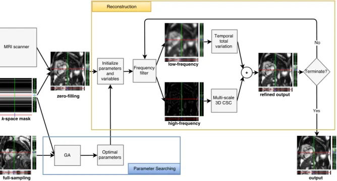
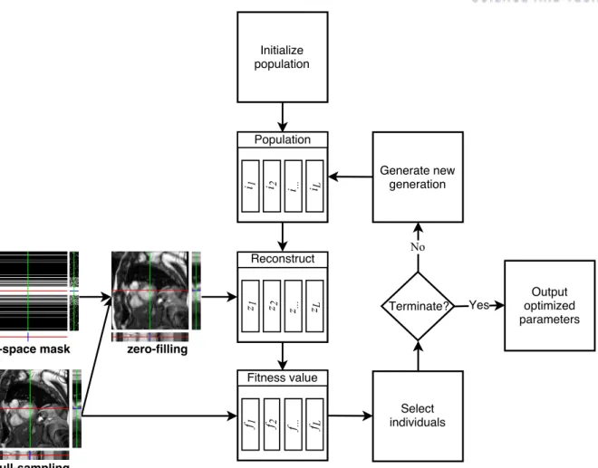
1 Overview of the proposed CS-MRI reconstruction process based on multi-scale 3D CSC with spectral decomposition and optimal parameter selection using a
genetic algorithm. . . 2
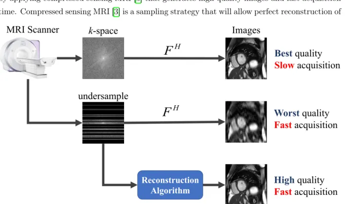
2 Overview of the CS-MRI problem. . . 3
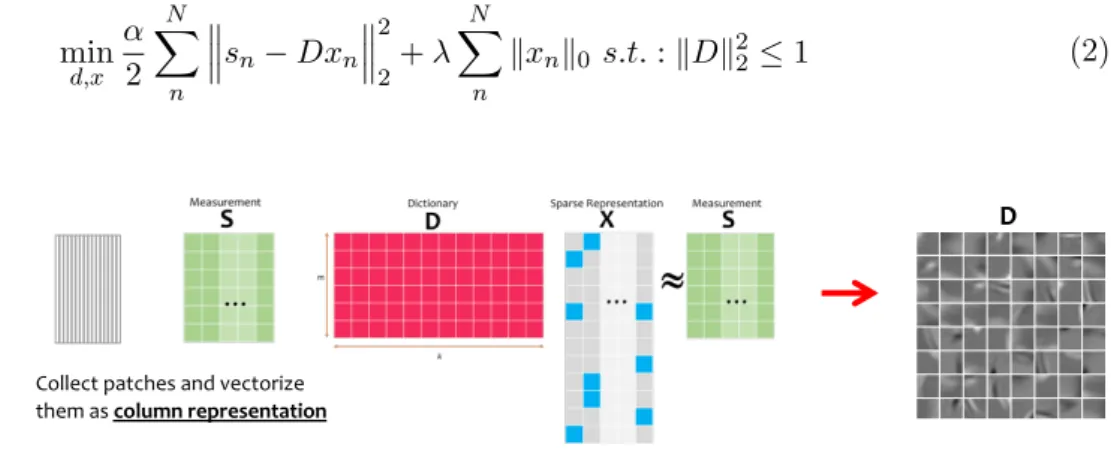
3 Overview of patch-based dictionary learning. . . 4
4 Overview of convolutional sparse coding. . . 4
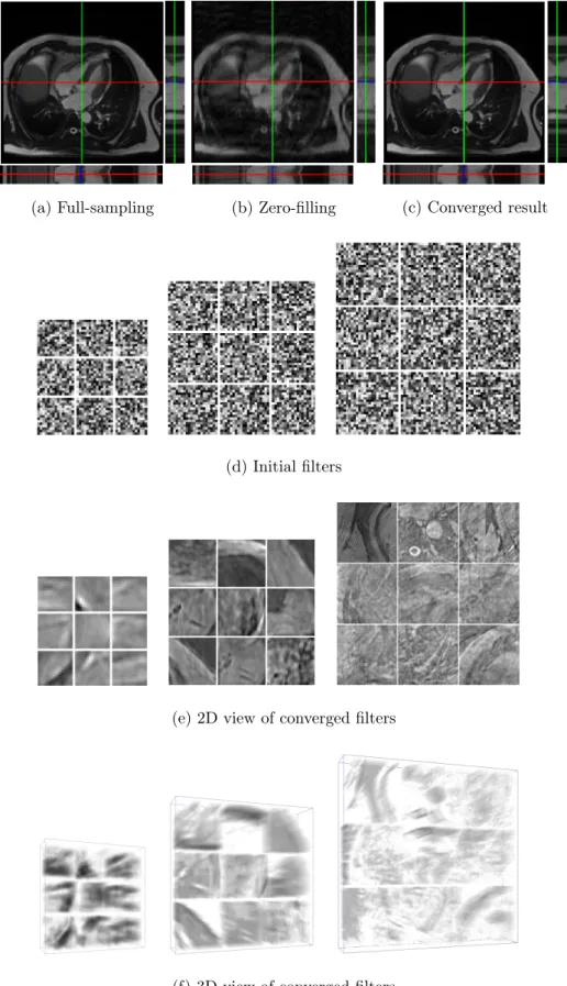
5 Overview multi-scale 3D CSC for CS-MRI reconstruction. . . 6
6 Genetic algorithm for automatically searching optimal parameters. . . 14
7 MRI datasets and Cartesian undersampling masks used in our experiments . . . . 20
8 MSEs, PSNRs, and SSIMs evaluation in three different sampling rates on cardiac MRIs (first column: MSEs; second column: PSNRs; third column: SSIMs). . . . 21
9 MSEs, PSNRs, and SSIMs evaluation in three different sampling rates on tumor DCE MRIs (first column: MSEs; second column: PSNRs; third column: SSIMs). 22 10 Image quality and pixel-wise error comparison of various reconstruction methods on Cardiac 2 dataset (12.5% sampling) . . . 23
11 Image quality and pixel-wise error comparison of various reconstruction methods on Tumor 2 dataset (12.5% sampling) . . . 24
12 Reconstruction quality comparison of Tumor 1 dataset . . . 25
13 PSNRs evaluation on the multi-coil MRI brain dataset . . . 26
14 Image quality and pixel-wise error comparison of multi-coil reconstruction meth-ods on the brain dataset (12.5% sampling) . . . 26
15 Average PSNRs of the images reconstructed from the various noise-corrupted k-space data . . . 27 16 Reconstruction of noise-corrupted Cardiac 3 dataset (at noise level 0.01) . . . 27 17 Reconstruction of noise-corrupted DCE tumor 3 dataset (at noise level 0.01) . . . 28 18 Convergence of proposed method for reconstructing 12.5% sampling Cardiac 1
dataset over 100 epochs. . . 29 19 Convergence rate comparison of 12.5% sampling Cardiac 2 and Tumor 2 datasets
in terms of PSNRs. . . 30 20 Convergence curves of 12.5% sampling cardiac and tumor data in terms of PSNRs
I Introduction
Dynamic magnetic resonance imaging (MRI), including dynamic contrast-enhanced (DCE) MRI and cardiac MRI, has been widely used to analyze changes in tissue characteristics or the move-ment of organs over time. Since dynamic MRI’s diagnostic performance is highly correlated with its temporal resolution [1], speeding up the acquisition time has been actively studied in the recent decades. More recently, compressed sensing theory [2] has been applied to the MRI reconstruction problem [3] to reduce the acquisition time. The objective of CS-MRI is to achieve close-to-perfect reconstruction from sub-Nyquist sampling [4] of k-space data from
the MRI scanner. [5] showed that the computational approach to CS-MRI can also accelerate conventional imaging. Slow numerical computation of CS-MRI reconstruction process can be further accelerated by leveraging parallel computing hardware such as graphics processing units (GPUs) [6].
Early work on CS-MRI exploited the sparsity of signal by applying universal sparsifying transforms such as the Fourier transform, total variation (TV) [7], and Wavelets [8]. For dy-namic CS-MRI, spatio-temporal correlations are commonly used (e.g., k-t FOCUSS [9, 10]).
Dictionary learning, a technique extracting common feature sets (i.e. atoms) from the training data, has been employed in CS-MRI to replace universal sparsifying transforms [11–15]. Since dictionary learning can generate custom-designed atoms that are better fit to the target image, reconstruction quality improves significantly compared to that of universal transforms. Recently, a filter-based dictionary learning method such as convolutional sparse coding (CSC) [16, 17], has been proposed to overcome the drawbacks of conventional patch-based dictionary learning, which includes generating redundant atoms and longer running time. CSC has been successfully adopted in solving dynamic CS-MRI problems [18, 19].
In this thesis, we introduce a novel dynamic CS-MRI reconstruction method that extends state-of-the-art CSC-based reconstruction methods [18,19]. First, we employ frequency filtering to separate low- and high-frequency components of the target image, and then use a relatively simple energy minimization process based on a temporal total variation (TV) energy for low-frequency reconstruction while more expensive feature encoding resources (i.e. dictionary of convolutional filters) are dedicated only to recovering high-frequency component of the image (see Fig. 1 for the overview of the reconstruction process). The motivation behind this approach is that, in conventional CS-MRI, low-frequencyk-space data is more densely sampled (see Fig. 7c k-space mask) while filter-based dictionary learning can better represent sparse local features
in high-frequency data. Second, we employ 3D convolutional filters in various scales and elastic net regularization [20] to further improve the reconstruction quality compared to conventional approaches that only use a single-scale dictionary andl1 regularization [15, 19]. Third, we
pro-pose an automatic optimal parameter-selection method based on a genetic algorithm (GA) for our iterative numerical solver, which is a variant of the alternating direction method of multipli-ers (ADMM). The proposed GA method belongs to the class of metaheuristics algorithms [21]
Figure 1: Overview of the proposed CS-MRI reconstruction process based on multi-scale 3D CSC with spectral decomposition and optimal parameter selection using a genetic algorithm. inspired by natural evolution to optimize objective function [22]. Our approach uses a GA only once to automatically find a set of optimal parameters without manual intervention, and then we can reuse them to reconstruct similar datasets. In our experiment on 15 cardiac and 7 dynamic contrast-enhanced (DCE) MRI datasets in three different Cartesian sampling rates (12.5%, 25% and 50%), the proposed reconstruction method produces significantly better image quality, com-pared to several state-of-the-art methods (e.g., k-t FOCUSS [9, 10], single-scale 3D CSC [19],
blind compressive sensing [13], patch-based dictionary learning [14,15], and FTVNNR [23]), and runs at an efficient rate with GPU acceleration.
The rest of the thesis is organized as follows. Section II illustrates the background knowl-edge included compressed sensing problem in dynamic MRI and dictionary learning algorithms. Section III reviews the recent literature related to the proposed method. Details of the proposed reconstruction process are introduced in Section IV. We demonstrate the performance of our reconstruction method and compare it with state-of-the-art methods in Section V. Finally, we summarize our work and propose future research directions in Section VI.
II Background
2.1 The Compressed Sensing In Dynamic MRI Problem
MRI scanner uses strong magnetic fields and radiofrequency pules to generate signals from body in frequency domain ( k-space) and images are created by taking inverse Fourier transform
magnetic fields of system need to align atoms inside organs and then the scanner records what happens as they relax back from excited state to unexcited state. In order to speed up the time of acquiring data, the scanner can only get a few samples despite of causing bad quality images ( see second row, Fig. 2). A good reconstruction method is used to overcome this drawback by applying compressed sensing MRI [3] that generates high quality images and fast acquisition time. Compressed sensing MRI [3] is a sampling strategy that will allow perfect reconstruction of
MRI Scanner
HF
Reconstruction Algorithm HF
k
-space
Images
Best
quality
Slow
acquisition
Worst
quality
Fast
acquisition
High
quality
Fast
acquisition
undersample
Figure 2: Overview of the CS-MRI problem.
discrete signal from a small number of samples. The dynamic MR data is obtained in frequency domain (k-space) as a sequence of 2D images (sfx⇥sfy) acquired atsft different time instances
which are stacked to become 3D volume sf. Thus, undersampling mask R is used to speed up
acquisition process by sampling m << sf k-space data. Given a sparsity transformation T,
the problem CSMRI can be expressed with 2D Fourier transformation for every instance F2 as
follow:
min
s kT(s)kp s.t.:kRF2(s) mk
2
2 < ✏2 (1)
where0p1and✏is a small constant representing for noise sampling ink-space. Generally,
an important of CSMRI is enforcing sparsity transformationkT(s)kp as much as possible. 2.2 Dictionary Learning Algorithms
Patch-based dictionary learning decompose patches of image into a linear combination
of overcomplete basis sets that provides sparse representation of this particular signal. The objective function Eq. 2 shows that the method collects patches and vectorize them as column representation. Output of this method is an approximation between dictionary D and sparse
mapx, as shown in Fig. 3. However, redundant of atom and slow running time are drawbacks
of this method because of using small patches for input.
min d,x ↵ 2 N X n sn Dxn 2 2+ N X n kxnk0 s.t.:kDk22 1 (2) D
Collect patches and vectorize
them as column representation
Figure 3: Overview of patch-based dictionary learning.
Convolutional sparse coding (CSC)is learning-based method that learns a shift-invariant
dictionary built by convolution filters from data. The brief overview of CSC is finding its best approximation image (s) from the summation of response map PNn dn⇤xn, shown in 3 .
min d,x ↵ 2 s N X n dn⇤xn 2 2+ N X n kxnk1 s.t.:kdnk22 1 (3)
Each response map is calculated by convolution between a filter (or atom)dn and sparse map
xn. The second non-linear norm term enforces sparsity to xn that helps finding a feasible
solution of collection dn and xn. The remaining constraint restricts the Frobenius norm of
each atom dn within a unit length. Zeiler et al. [24] proposed a solution by solving series
of subproblems between dn and xn until convergence; however, performance is significantly
affected by complexity convolution operator because the solvers is completely on image domain. The efficient approaches [7, 16, 25] to solve Eq. 3 leverages Fourier Convolution theorem that convolution operator on spatial domain is equivalent to element-wise on frequency domain. For example, Fig. 4 shows that features are extracted by using convolutional sparse coding.
≈
∑
k=1 K∑
k=1 K*
dk xk≈
DIII Related work
Since its inception in [3]’s seminal work, CS-MRI has been actively studied to accelerate the time-consuming MRI imaging process. Conventional CS-MRI algorithms are mainly based on promoting sparsity in the data by employingl1regularization in universal sparsifying
transforma-tion models. In such methods, the target image is transformed into a sparse domain by applying universal transforms such as Wavelet and Fourier transforms or total variation operation [26,27]. CS-MRI for dynamic data is also proposed by enforcing spatial and temporal coherence (i.e.,
k-t FOCUSS [9, 10] and [28]). These conventional CS-MRI methods suffer from computational
overhead because of solving expensive nonlinear l1 minimization problems. This leads to the
development of efficient numerical algorithms [29, 30] that leverage the Alternating Direction Method of Multipliers (ADMMs) to solve this nonlinear problem in CS-MRI [6]. CS-MRI re-construction methods using nuclear norm and low-rank matrix completion techniques [23,31–35] have also been proposed.
More recently, while the major limitation of universal transform-based methods is just using transformation in general, dictionary learning (DL) [36], an unsupervised learning approach, can be adapted to features from input data by training dictionary. Thus, conventional DL in CS-MRI [11–15] approaches have successfully applied to enhancing MRI reconstruction quality. Caballero et al. [14, 15], for instance, demonstrated the efficiency of using patch-based DL for dynamic MRI reconstruction with temporal TV filter for enforcing coherence of time-axis. Efficient convolutional sparse coding (CSC) is then introduced by minimizing an energy objective function using a convolutional operator on the image domain, which leads to element-wise in the frequency domain, derived within ADMMs framework [16, 17, 25]. [18, 19] first employed CSC to solve CS-MRI problems, which significantly improves running time and reconstruction quality by building more compact and expressive shift-invariance convolutional filters. Nevertheless, MR data contains various feature sizes so that multiple dictionary sizes in the multi-scale 3D CSC method can adapt well to the data rather than single-scale atom size methods (e.g., [13,15,19]). The multi-scale 3D CSC in our method builds the dictionary by simultaneously learning shift-invariant multiple sizes of convolutional filters from data (Fig. 5). In this approach, zero-filling (Fig. 5b, zero-filling reconstruction) and randomly initialized filters (e.g., in Fig. 5d, the various filter sizes) are updated iteratively until they converge, as shown in Fig. 5c, 5e, and 5f.
There are a few approaches that leverage different reconstruction strategies based on the frequency range of the image. [37] proposed a two-stage reconstruction method which performs the first-step reconstruction of low-frequency component only from the central region ofk-space
data, and then combines this result with the remaining k-space data (corresponding to
high-frequency component) to conduct the second-step reconstruction from the full k-space data. A
filter-based reconstruction approach [38] separates k-space with high- and low-pass filters,
re-constructs each frequency component independently, and combines the reconstructed results to generate the final image. Our method shares a similar idea with these previous work by
split-(a) Full-sampling (b) Zero-filling (c) Converged result
(d) Initial filters
(e) 2D view of converged filters
(f) 3D view of converged filters
Figure 5: Overview multi-scale 3D CSC for CS-MRI reconstruction.
ting k-space (i.e. frequency) data, but our method employs advanced reconstruction methods
sparsity in high-frequency and temporal TV for coherency in low-frequency). Furthermore, our method iteratively updates the result to enforce the measurement consistency (see Algorithm 1 and the constrain term in Eq. 7) while the other methods perform one-time reconstruction for each frequency data and then combining them.
Genetic algorithm (GA) is a population-based method which is inspired by nature’s capability to evolve living beings well-adapted to their environment [21,39]. This meta-heuristic algorithm, which is well known in optimization problem with many applications [21, 22, 39], deals in every iteration with a set of solutions rather than with a single solution (i.e. hill-climbing, simulated annealing and tabu search). The main idea of GA is generating a sequence of populations (i.e. generations) where each individual in a population is a solution to the problem. A new generation is created from the previous generation using natural operations such as mutations and crossovers based on the fitness values from members of the current population. This evolution process stops when the number of generations is greater than the pre-defined number and outputs an individual which has a minimum fitness value. Meta-heuristics in optimization is an immense research field and many different classes of algorithms exist, such as single-state methods, population methods, and hybrid methods [21,39]. To the best of our knowledge, our approach is the first attempt to use GA for automatic parameter selection in the CS-MRI reconstruction problem.
IV Proposed Method
The overview of our proposed CS-MRI reconstruction process is illustrated in Fig. 1. The input to our method is a zero-filling reconstruction that is generated by applying inverse Fourier transform to the undersampled k-space data from the MRI scanner, which suffers from undersampling
artifacts. Then, the proposed method consists of two components: the reconstruction process
that takes a zero-filling reconstruction as an initial guess to improve image quality (i.e. removing undersampling artifact, Fig. 1 yellow box), and the parameter searching process using a GA (Fig. 1 blue box).
4.1 Reconstruction Process
In the reconstruction process, the input zero-filling reconstruction image is separated into low-and frequency zero-filling images by applying a blow-and-pass frequency filter. The high-frequency image is then reconstructed by using multi-scale 3D CSC with elastic net regular-ization. This multi-scale CSC method adapts well to features of various sizes, and elastic net regularization can outperform l1-only regularization without impairing the sparsity of
repre-sentation [20]. In the meantime, the low-frequency image is reconstructed by minimizing the total variation along the temporal direction (i.e., promoting sparsity in the temporal gradient field), which is based on the observation that the information in dynamic MRI data is sparser in first-order temporal gradients than in spatial gradients [15]. At the end of the reconstruction process, the reconstructed low- and high-frequency images are combined together to generate
a refined output (i.e. undersampling artifact is reduced). This update process is repeated (see Algorithm 1) until reaching the stopping criteria in which the number of iterations are greater than a pre-defined number, or primal and dual residuals are less than an absolute value, as discussed in Sec. 3.3 of [30]. More detailed discussions of the proposed method are presented in the following sections.
Algorithm 1 Iterative reconstruction process using spectral decomposition
1: procedureReconstruction(m) . m: sparse measurement ofk-space
2: s0 F2H(m) .input: zero-filling reconstruction
3: whilestopping criteria not met do
4: sl
i =F2HHF2(si) . H: low-pass filter;F2: 2D Fourier transform
5: shi =si sli
6: sli+1 findsli+1 in minimizing temporal TV problem .Eq. 8
7: sh
i+1 findshi+1 in multi-scale 3D CSC problem . Eq. 12
8: si sli+1 +shi+1
9: returnsi . si with removed artifact
Spectral decomposition using a frequency filter
To apply different reconstruction strategies based on the frequency range, we decompose the input image into low- and high-frequency images by applying a two-dimensional Butterworth low-pass filter (BLPF) to every 2D MRI slice in the frequency domain. The transfer function
H(u, v)of the BLPF of ordernwith a cutofffrequency at a specified distanceD0 from the origin
is defined as follows:
H(u, v) = 1
1 + [D(u, v)/D0]2n (4)
where D(u, v) is the distance from a point (u, v) to the center of the frequency domain, and
the parameters D0 and n define how the frequency is cut off. Thus, for the input images, the
low-frequency image sl can be computed using two-dimensional Fourier transform F2 and its
inverse FH
2 along the time-axis as follows:
sl=F2HHF2(s) (5)
and the high-frequency image sh can be computed as follows:
sh =s sl (6)
The choice ofD0andncan be automatically made via our proposed parameter selection method
Temporal total variation and multi-scale 3D CSC for reconstruction
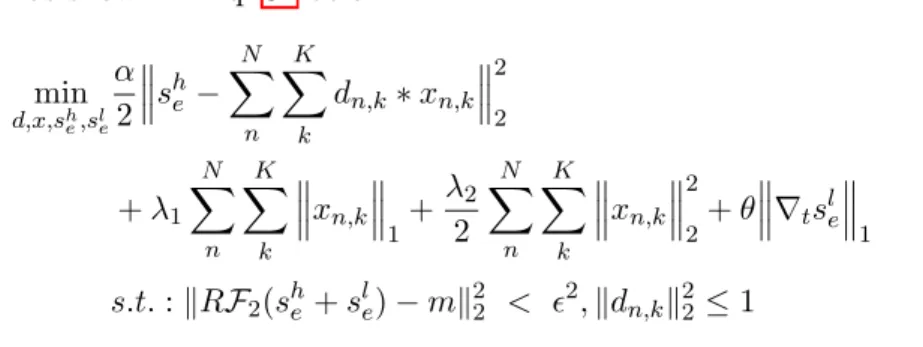
After the frequency filter splits the input imagesinto high(sh)and low(sl)frequency images, the
reconstruction process reduces undersampling artifact in sby solving the energy minimization
problem as follows: min d,x,sh,sl ↵ 2 s h N X n K X k dn,k⇤xn,k 2 2 + 1 N X n K X k xn,k 1+ 2 2 N X n K X k xn,k 2 2+✓ rts l 1 s.t.:kRF2(sh+sl) mk22 < ✏2,kdn,kk22 1 (7)
where N is the number of filter scales (i.e. levels), K is the number of filters in each scale, ⇤ is a convolution operator, dn,k is the k-th filter (or atom) in nth dictionary (i.e. dictionary
for level n), and xn,k is its corresponding sparse code (or sparse map) for sh. Note that the
dimension of the filters we used were 15⇥15⇥20, 20⇥20⇥25, and 25⇥25⇥30, and the
dimension of the sparse map xn,k was identical to the size of the image. In Eq. 7, the first
term measures the difference between sh and its sparse approximation sh P Pd
n,k⇤xn,k,
weighted by ↵. The combination of the second and third terms, which are weighted by 1 and 2 parameters, are called elastic net regularization [20]. The fourth term✓krtslk1 is the total
variation energy that enforces the temporal coherence of the low-frequency image. The rest of this equation is the collection of constraints: the first constraint keeps the consistency between undersampled measurement m and the undersampled reconstructed image using k-space mask RwithF2 operator; the second constraint restricts the Frobenius norm of each atomdn,k within
a unit length. In following discussion, we simplify the notations without indices n,k and also
replace the result of Fourier transform of a given variable by using subscript f (for instance, df3 represents simplified notation for F3d in the 3D domain and s
h
f2 is the simplified notation
for F2sh in the 2D spatial domain). The problem (7) can be split into two sub-optimization
problems as follows, which can be iteratively updated for the global minimum solution.
Temporal TV minimization: we minimize Eq. 7 with respect to sl, which contains the
total variation along the time-axis and the measurement constraint term.
min sl ✓krts lk 1 s.t.:kRF2(sh+sl) mk22 < ✏2 (8) Eq. 8 can be written in an unconstrained form with parameter, as shown in Eq. 9 below:
min sl ✓krts lk 1+ 2kRF2(s h+sl) mk2 2 (9)
method [40]. sl(i+1)= 2F H 2 ml rTtz(i) z(i+1)=clip(z(i)+ 1 ⌘rts l (i+1), ✓ 2) (10) whereml is equal tom RF2sh andiis the iteration number. The clipping function is defined
in Eq. 11. clip(a, b) = 8 < : a, if |a|b b·sign(a), if |a| b (11)
The index i starts with 0, the initial z(0) = 0, and ⌘ maxeig(rtrT
t). In this case, the
maximum eigenvalue of rtrT
t is less than four regardless to the length of signal; thus, we can
set⌘= 4and the maximum number of iterations equals 40 in our experiments. Note that✓and
are optimized by using a GA (see Section 4.3). For more details on parameter and derivation about the algorithm, refer to [40]
Multi-scale 3D CSC with elastic net regularization: in this problem, we find sh in
the energy minimization function, as follows:
min d,x,sh ↵ 2 s h N X n K X k dn,k⇤xn,k 2 2 + 1 N X n K X k xn,k 1+ 2 2 N X n K X k xn,k 2 2 s.t.:kRF2(sh+sl) mk22 < ✏2,kdn,kk22 1 (12)
Eq. 12 can be re-written using auxiliary variablesy and g forx and d, as follows: min d,x,g,y,sh ↵ 2 s h X Xd⇤x 2 2+ 1kyk1+ 2 2 kyk 2 2 s.t.:x y= 0,kRF2sh mhk22 < ✏2, g=P roj(d),kgk22 1 (13) where mh is equal to m RF
2sl. The g and d variables are related by a projection operator
as a combination of a truncated matrix with the corresponding dictionary size followed by a padding-zero in oder to make the dimension of g the same as that of x, and the variable g
should also be zero-padded to make its size similar to gf3 and xf3 so we can leverage Fourier
transform to solve this problem. The constrained Eq. 13 can be unconstrained by using dual variableu,h, and further regulates the measurement consistency and the dual differences with
,⇢ and , respectively: min d,x,g,y,sh ↵ 2 s h X Xd⇤x 2 2+ 1kyk1+ 2 2 kyk 2 2 + 2kRF2s h mhk2 2+ ⇢ 2kx y+uk 2 2 + 2kd g+hk 2 2 s.t.:g=P roj(d),kgk22 1 (14)
We solve Eq. 14 by iteratively finding the minimization solution of subproblems, as shown below: Solve forx: min x ↵ 2 X X d⇤x sh 2 2+ ⇢ 2kx y+uk 2 2 (15)
We apply the Fourier transform to subproblem (15), it becomes:
min xf3 ↵ 2 X X df3xf3 s h f3 2 2+ ⇢ 2kxf3 yf3 +uf3k 2 2 (16)
Next, the minimum solution can be found by taking the derivative of Eq. 16 with respect to variablexf3 and setting it to zero. The solution is shown in Eq. 17.
(↵DHf3Df3+⇢I)xf3 =D
H
f3s
h
f3+⇢(yf3 uf3) (17)
whereDf3 is the concatenation of all diagonalized matricesdf3 n,k, as illustrated in Eq. 18 and
DHf3 is the Hermitian transpose ofDf3.
Df3 = [diag(df3 1,1), ..., diag(df3 1,k), ..., diag(df3 n,k)] (18)
Solve fory: min y 1kyk1+ 2 2 kyk 2 2+ ⇢ 2kx y+uk 2 2 (19)
In [16–19],l1 regularization is only used for CSC; however, our subproblem contains both lasso
and ridge regularizations. Fortunately, this subproblem can also be solved by using a shrinkage operation: y =S 1/( 2+⇢)⇣⇢(x+u) 2+⇢ ⌘ (20) Update foru:
The update rule for u can be defined as a fixed-point iteration with the difference between x
and y (u converges whenx and y converge each other).
u=u+x y (21) Solve ford: min d ↵ 2 X X d⇤x sh 2 2+ 2kd g+hk 2 2 (22)
We solve this subproblem in the Fourier domain, similar tox: min df3 ↵ 2 X X df3xf3 s h f3 2 2+ 2kdf3 gf3 +hf3k 2 2 (23) (↵XfH3Xf3+ I)df3 =X H f3s h f3+ (gf3 hf3) (24)
Note that Xf3 stands for the concatenated matrix of all diagonal matrices xf3 n,k as shown in
Eq. 25 andXfH3 is the Hermitian transpose ofXf3.
Solve forg:
min
g 2kd g+hk
2
2 s.t.: g=P roj(d),kgk22 1 (26)
g can be solved by using the inverse Fourier transform of df3. This projection should be
con-strained by suppressing the elements which are outside the filter size dn,k, and followed by
normalizing itsl2-norm to a unit length.
Update forh: Similar to u, we update h as follows:
h=h+d g (27) Solve for sh: min sh ↵ 2 s h X Xd⇤x 2 2+2kRF2s h mhk2 2 (28)
Subproblem (28) can be transformed and solved in the 2D Fourier domain:
min sh f2 ↵ 2 s h f2 F H 2 X X df3xf3 2 2+2kRs h f2 m hk2 2 (29)
Previously,df3 andxf3 were obtained in the 3D Fourier domain, we must bring it onto the same
space by applying an inverse Fourier transform along the time-axis F2H. Finally, shf2 can be
found by solving the following linear system:
( RHR+↵I)shf2 = RHmh+↵F2HX Xdf3xf3 (30)
Note that we can efficiently solve independent linear systems (17), (24), and (30) via the Sherman-Morrison formula, as shown in [17]. After the iteration process, sh will be the
re-sults of applying a 2D inverse Fourier transform F2H to shf2.
4.2 Complexity analysis of proposed reconstruction algorithm
Our iterative method consists of spectral decomposition using low-pass filter and solving sub-problems. In order to investigate computational complexity, we will carefully analyze these components using Big O Notation, as shown in Table 1. Suppose P is the number of pixels in
dynamic MR image and M is total convolutional filters (M =N ⇥K). Firstly, the cost of fast
Fourier transforms (FFTs) of the MR image isO(P logP). In spectral decomposition step,
low-pass filter is used to separate spectral of MR data which costs O(P); however, this step needs
FFTs operator so it costsO(P logP). Temporal TV minimization (sl) contains FFTs, calculating
temporal TV and clipping operator which cost O(P logP), O(P) and O(P), respectively. For
solving subproblemsx,dandsh (Eq. 17, 24 and 30), these can be efficiently solved by
Sherman-Morrison formula withO(M P)cost proposed by [25] so that the dominant operator is FFTs at
all M indicesO(M P logP). The same computational complexityO(M P logP)can be interpreted
for solving subproblemg because of domination of FFTs operator. Finding solution for y using
shrinkage operation which is applied for every element in y; thus, it cost O(M P). Finally,
the addition and subtraction operations for updating u and h cost O(M P). In conclusion, the
Component Complexity
Spectral decomposition (Eq. 4) O(P logP)
Solvesl (Eq. 10) O(P logP)
Solvex, d and sh (Eq. 17, 24 and 30) O(M P logP)
Solveg O(M P logP)
Solve y (Eq. 20) O(M P)
Update uand h (Eq. 21 and 27 ) O(M P)
Table 1: Complexity analysis of proposed method.
4.3 Parameter Searching Process
The proposed reconstruction process contains many user-controllable parameters (e.g., ↵, ,
1, 2, ⇢, , ✓,D0 and n), and manually adjusting these parameters is a time-consuming and
laborious process. Thus, we propose an automatic parameter searching process, which can be thought of as a pre-processing step of the reconstruction process. Our searching approach employ a GA, which is a meta-heuristic algorithm inspired by the process of natural evolution, as shown in Fig. 6. In the proposed parameter searching process, we create a simulation based on the objective function which is defined by a fully-sampledk-space data and an undersampling mask,
and a GA finds the best parameters to minimize this objective function.
A detailed description of the parameter selection process is introduced below. First, the full (ground-truth) image is undersampled to generate zero-filling reconstruction using the same sampling mask used in the reconstruction process. Then, GA arbitrarily initializes a population with L members where each individual (i) has a set of nine randomly chosen parameters to be used in the reconstruction process. Next, the zero-filling is reconstructed L times by using our method (Fig. 1 yellow box) that each time uses a set of nine parameters which contents in every individual (i) of the current population to get reconstructed results (z). The fitness values of objective function f are then calculated for each member in the current population by comparing between the full-sampled and reconstructed image (z) as well as sparse code x.
After ward, GA selects members, called parents, based on the ranking of their calculated fitness values. Finally, there are three types of children that are generated for the next generation such as elite children with the best fitness values, crossover children created by combining a pair of parents and mutation children created by introducing random changes to a single parent. The algorithm continues by creating a loop of generating the new generation based on bio-operators until reaching the terminate condition (i.e., the current generation is greater than pre-defined number). In general, the goal of GA in optimization problem is conducting many trials and errors to find the best individual which minimizes the fitness function. Therefore, we propose a fitness function(f), as shown in Eq. 31, that uses Peak Signal-To-Noise-Ratio (P SN R) between
Figure 6: Genetic algorithm for automatically searching optimal parameters.
↵ 1 2 ⇢ ✓ D0 n
Lower 0.001 0.001 0.001 0.001 1 1 0.001 1 1 Upper 5 5 5 5 100 100 1 5 5 Table 2: Lower and upper bounds of parameters used in our experiment. which are outputs of the reconstruction process (Fig. 1 yellow box) after 100 iterations.
f = P SN R+⌧x¯ (31)
where⌧ is the weight for trade-off between 2 values P SN R (bigger is better) and average of x
(smaller is better). Moreover, we also set possible lower and upper bounds for each parameter to narrow down the GA’s searching space, as illustrated in Table 2. Specially, our experiment shows that a GA can be applied only once to find the optimal parameters that work for similar types of data (i.e., cardiac or DCE MRI data).
V Experiment Results
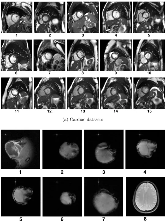
To assess the performance of our method, we conducted experiments on 15 cardiac MRI datasets from The Data Science Bowl [41] (30 frames of a 256⇥256 image across the cardiac cycle of a heart for each dataset), 7 tumor DCE MRI datasets (128⇥128 image with 128 frames of each
dataset) and a multi-coil MRI brain dataset [42] (128⇥128 with 12 frames in which each frame consists of 12 parallel acquisitions) in three different rates of Cartesiank-space undersampling
masks (12.5%, 25% and 50% sampling masks), as shown in Fig. 7c. GA is also set to run only one time to search parameters in five generations withL= 200 and⌧ = 20. More specifically, for each
kind of dataset, we arbitrarily select one full-sampled data and the sampling mask to optimize parameters, and reuse these found parameters to reconstruct the remaining of MRI datasets. We compare our method with several state-of-the-art methods, including k-t FOCUSS [10],
FTVNNR [23], BCS [13], Caballero et al. [15], and 3D CSC [19]. We also compare with the intermediate versions of our method (i.e., incrementally adding new features, such as multi-scale extension of CSC, elastic net regularization, and spectral decomposition, to the baseline version of 3D CSC [19] to assess how each addition of feature affects the overall performance of the method (see Table 3). The proposed prototype system is implemented using MATLAB 2017a with GPU support.
Method Abbreviation
k-tFOCUSS [10] k-t FOCUSS
Algorithm using low-rank and
total variation regularizations [23] FTVNNR Blind compressive sensing [13] BCS
DLTG [15] DLTG
3D CSC [19] 3D-CSC
Multi-scale 3D CSC Multi-scale Multi-scale 3D CSC withl1, l2 regularization Elastic multi-scale
Elastic multi-scale and temporal TV minimization Elastic multi-scale tv Elastic multi-scale on high-frequency, and
temporal TV minimization on low-frequency Our method Table 3: CS-MRI reconstruction methods compared in our experiment.
5.1 Reconstruction quality evaluation
For a fair comparison, we set up all DLTG [15] and CSC methods with the same number of filters (27 filters). All multi-scale 3D CSC methods used three different filter sizes (N = 3) and each
of Mean Square Errors (M SEs), Peak Signal-To-Noise-Ratios (P SN Rs) and Structural
SIM-ilarities (SSIM s) for cardiac and tumor DCE MRIs; on each box, the central mark indicates
the median, and the bottom and top edges of the box indicate the 25th and 75th percentiles, respectively. As can be seen in Fig. 8 and 9, our method gives a higher P SN R, SSIM and
a lower M SE compared to the other approaches in case of 12.5%, 25%, 50% sampling rates.
Fig. 10 and 11 show a qualitative comparison of various reconstruction results. It is shown that our method generates less visual artifact compared to other methods (see the region of inter-ests and pixel-wise error maps), even under an extremely low sampling rate (12.5%). It is also worth noting that our method can reconstruct temporal changes in DCE data more accurately compared tok-t FOCUSS and DLTG at a very low sampling rate (see Fig. 9 12.5%).
The Akep value, borrowed from the [43]’s model, is also a commonly used quality metric for
dynamic MRI (especially DCE) to judge the consistency of the reconstructed image sequence because this value reflects the degree of MRI signal enhancement and the exchange rate in term of brightness and the contrast. Therefore, Akep value characterizes the velocity of MRI
signal change in the region of interest (ROI) of the tumor, which is shown to provide the relevant information regarding tumor perfusion and permeability. To assess how the proposed reconstruction method performs, we measure the Akep on each reconstructed image (actually,
Akep is generated per pixel) and generate a least-square fitting curve. By comparing the curve’s
shape, we can verify the reconstruction method’s efficacy. The Fig. 12a shows Akep values as a
color map of Tumor 1 dataset in Fig. 7b where our result clearly preserves details much better than the others and Fig. 12b and 12c shows the curve fitting profiles at some locations (marked A and B in Fig. 12a). As illustrated, our curve fitting profiles closely approximate the ground truth (full signal). In addition, our method effectively reduces the intensity variation (or noise) of the reconstructed images (see the variation of red circles are much smaller than that of other results) due to enforcing temporal coherence using a TV energy.
Overall, the proposed method achieves better reconstruction quality than other state-of-the-art methods. Shift-invariant convolution filters can represent both spatial and temporal features well, whilst multi-scale 3D CSC withl1 andl2 regularization shows its performance with better
M SE, P SN R and SSIM. Moreover, our frequency-splitting reconstruction approach, using
temporal TV minimization for low-frequency and multi-scale 3D CSC with elastic net regular-ization for high-frequency, can significantly improve the image quality as well as convergence rate, which will be discussed in Section 5.4.
5.2 Extension to multi-coil parallel MR
Although we introduced our method for single coil MRI data in the previous sections, the proposed method can be applied to multi-coil MRI data as well with a small modification. For this, the main objective function (Eq. 7) can be combined with SENSE in the k-t
Fourier transform as shown in Eq. 32 below: min d,x,sh e,sle ↵ 2 s h e N X n K X k dn,k⇤xn,k 2 2 + 1 N X n K X k xn,k 1+ 2 2 N X n K X k xn,k 2 2+✓ rts l e 1 s.t.:kRF2(she +sle) mk22 < ✏2,kdn,kk22 1 (32) wheresh e =Esh andsle=Esl.
We tested the parallel version of our method on a 12-coil MRI brain dataset, and compared with FTVNNR, BCS and 3D-CSC methods for image quality assessment. For all sampling rates we tested (12.5%, 25% and 50%), our method outperformed the other methods (i.e., higher PSNR of reconstructed images, see Fig. 13a and Fig. 13b). Fig. 14 also shows that our method is less prone to pixel-wise errors and generates images closer to the full reconstruction than FTVNNR, BCS and 3D-CSC.
5.3 Robustness to noise
Noise resiliency is another important quality measure for the MR image reconstruction algorithm. To assess the noise resiliency of the proposed method, we synthetically corrupted the undersam-pled k-space data with Gaussian random noise and compared the reconstruction quality. In this experiment, we used cardiac and DCE MRI datasets at three Cartesian sampling rates, cor-rupted with Gaussian white noise in various levels (the range of standard deviation of Gaussian is {0.01, 0.03, 0.05, 0.07, 0.09, 0.1}), as shown in Fig. 7c. We compared the reconstruction results with those of three representative methods (FTVNNR [23], BCS [13] and 3D-CSC [19]) because they represent general transformation (non-learning approach), patch-based dictionary learning, and convolutional sparse coding, respectively. The optimal parameters found in the previous experiments (Sec. 5.1) are used for all methods in this experiment. As shown in Fig. 15, 16 and 17, our method produced the results with much higher PSNR, less noise, and superior image quality compared to the other methods.
5.4 Convergence evaluation
Fig. 18 illustrates the convergence of our method over 100 iterations. The left column contains full low-frequency, full high-frequency, full reconstruction and total time-axis gradient value of full low frequency, whilst right column gives the changing of refined output with its low- and high-frequency as well as the convolutional filters and temporal total variation value. In Fig. 18, the features in high-frequency part are progressively refined along with converging of convolutional filters every twenty epochs. The temporal total variation value in low-frequency also reduces over iterations which enforces the coherence of time-axis. As seen in Fig. 19 and 20, using temporal TV minimization is clearly helpful for the reconstruction process, while our frequency splitting
approach can significantly improve the quality with comparable convergence rate. The proposed method converges faster (i.e. require less number of epochs) than 3D-CSC, multi-scale and elastic multi-scale. Note that patch-based dictionary (DLTG [15]) usually converges faster, but the actual running time is much slower because there is no GPU acceleration as in our method (see Table 4). Moreover, Fig. 19 and 20 show adequate convergence curves of the CSC methods with a large P SN R improvement and no divergence. Thus, GA can find optimal parameters
for the reconstruction process. In our observation, when we used the searched parameters for all datasets in the same kind of MRIs, the efficiency of convergence rate still remains, as shown in Fig. 20.
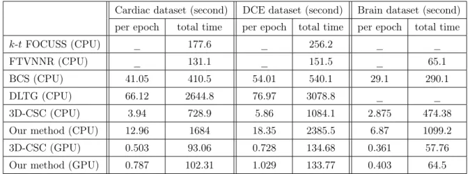
5.5 Running time evaluation
We measured the average reconstruction time of methods on a PC equipped with an Intel i7-7700K CPU and a NVIDIA Titan X GPU. All CSC approaches and DLTG [15] were run for 200 epochs, as shown in Fig. 19 and 20; however, the rate of convergence varied over methods. For example, our method converged in about 130 epochs, while DLTG took about 40 epochs (see Fig. 19) and 3D-CSC took more than 185 epochs (see Fig. 20). As shown in Table 4, the average per-epoch running time of our method on a GPU is 36.9⇥, 84⇥, 5⇥, and 16.5⇥faster
than BCS, DLTG, 3D-CSC (CPU) and the CPU version of our method, respectively. A similar performance gain of our method was observed on DCE MRI data and multi-coil brain MRI date as well. Furthermore, DLTG converged faster (i.e., small number of epochs) than our method, but the actual running time of our method on a GPU to reach the convergence was significantly faster than that of DLTG (speed up of 25.58⇥for cardiac and 23⇥for DCE data). However, due
to the computational overhead of our method (e.g., frequency filtering and energy optimization in low- and high-frequency), single-scale 3D CSC on a GPU was faster than our method. We also expect a significant performance improvement using NVIDIA CUDA and C/C++ over the current implementation using MATLAB, which is left for the future work.
Cardiac dataset (second) DCE dataset (second) Brain dataset (second)
per epoch total time per epoch total time per epoch total time
k-tFOCUSS (CPU) _ 177.6 _ 256.2 _ _
FTVNNR (CPU) _ 131.1 _ 151.5 _ 65.1
BCS (CPU) 41.05 410.5 54.01 540.1 29.1 290.1
DLTG (CPU) 66.12 2644.8 76.97 3078.8 _ _
3D-CSC (CPU) 3.94 728.9 5.86 1084.1 2.875 474.38
Our method (CPU) 12.96 1684 18.35 2385.5 6.87 1099.2
3D-CSC (GPU) 0.503 93.06 0.728 134.68 0.361 57.76
Our method (GPU) 0.787 102.31 1.029 133.77 0.403 64.5
Table 4: Average running time of various reconstruction methods (per epoch: average running time of one epoch; total time: average running time to reach the convergence).
VI Conclusion and Future Work
In this thesis, we introduced a novel CS-MRI reconstruction workflow based on an unsuper-vised learning approach. We discovered that the frequency-dependent reconstruction, i.e., using temporal total variation for low-frequency reconstruction and multi-scale 3D CSC with elastic net regularization for high-frequency reconstruction, played an important role for improving the overall reconstruction quality and the convergence rate. We also analyze computational com-plexity of our reconstruction algorithm. The proposed automatic parameter searching method using GA significantly reduced user’s effort for tuning parameters in the reconstruction process. Furthermore, we showed that the proposed method can be easily extended to parallel MR imag-ing. The results showed that the proposed method outperformed the state-of-the-art CS-MRI reconstruction methods, such as k-t FOCUSS [9, 10], FTVNNR [23], single-scale 3D CSC [19],
blind compressive sensing [13] and patch-based dictionary learning [14, 15], in terms of image quality and noise resiliency. In the future, we plan to improve the speed of proposed method by leveraging the parallel computing technology, such as multi-GPU and cluster systems. Explor-ing advanced meta-heuristic algorithms to improve the parameter selection process is another interesting future research direction.
(a) Cardiac datasets
1 2 3 4
5 6 7 8
(b) Tumor DCE (1-7) and multi-coil brain (8) datasets
(c) Undersamplingk-space masks
Zero-fillingk-t FOCUSS DLTG FTVNNR BCS 3D-CSC Multi-scale Elastic multi-scale Elastic multi-scale tv Our method 0 0.5 1 1.5 2 2.5 3 12.5% sampling Zero-fillingk-t FOCUSS DLTG FTVNNR BCS 3D-CSC Multi-scale Elastic multi-scale Elastic multi-scale tv Our method 20 22 24 26 28 30 32 34 12.5% sampling Zero-fillingk-t FOCUSS DLTG FTVNNR BCS 3D-CSC Multi-scale Elastic multi-scale Elastic multi-scale tv Our method 0.5 0.6 0.7 0.8 0.9 12.5% sampling Zero-fillingk-t FOCUSS DLTG FTVNNR BCS 3D-CSC Multi-scale Elastic multi-scale Elastic multi-scale tv Our method 0 0.1 0.2 0.3 0.4 0.5 0.6 0.7 0.8 25% sampling Zero-fillingk-t FOCUSS DLTG FTVNNR BCS 3D-CSC Multi-scale Elastic multi-scale Elastic multi-scale tv Our method 26 28 30 32 34 36 38 25% sampling Zero-fillingk-t FOCUSS DLTG FTVNNR BCS 3D-CSC Multi-scale Elastic multi-scale Elastic multi-scale tv Our method 0.7 0.75 0.8 0.85 0.9 0.95 25% sampling Zero-fillingk-t FOCUSS DLTG FTVNNR BCS 3D-CSC Multi-scale Elastic multi-scale Elastic multi-scale tv Our method 0 0.02 0.04 0.06 0.08 0.1 0.12 0.14 0.16 50% sampling (a) MSEs Zero-fillingk-t FOCUSS DLTG FTVNNR BCS 3D-CSC Multi-scale Elastic multi-scale Elastic multi-scale tv Our method 32 34 36 38 40 42 44 46 50% sampling (b) PSNRs; unit:dB Zero-fillingk-t FOCUSS DLTG FTVNNR BCS 3D-CSC Multi-scale Elastic multi-scale Elastic multi-scale tv Our method 0.9 0.92 0.94 0.96 0.98 1 50% sampling (c) SSIMs
Figure 8: MSEs, PSNRs, and SSIMs evaluation in three different sampling rates on cardiac MRIs (first column: MSEs; second column: PSNRs; third column: SSIMs).
Zero-fillingk-t FOCUSS DLTG FTVNNR BCS 3D-CSC Multi-scale Elastic multi-scale Elastic multi-scale tv Our method 0 0.2 0.4 0.6 0.8 1 1.2 1.4 1.6 1.8 12.5% sampling Zero-fillingk-t FOCUSS DLTG FTVNNR BCS 3D-CSC Multi-scale Elastic multi-scale Elastic multi-scale tv Our method 25 30 35 40 12.5% sampling Zero-fillingk-t FOCUSS DLTG FTVNNR BCS 3D-CSC Multi-scale Elastic multi-scale Elastic multi-scale tv Our method 0.5 0.6 0.7 0.8 0.9 1 12.5% sampling Zero-fillingk-t FOCUSS DLTG FTVNNR BCS 3D-CSC Multi-scale Elastic multi-scale Elastic multi-scale tv Our method 0 0.1 0.2 0.3 0.4 0.5 0.6 0.7 0.8 25% sampling Zero-fillingk-t FOCUSS DLTG FTVNNR BCS 3D-CSC Multi-scale Elastic multi-scale Elastic multi-scale tv Our method 25 30 35 40 45 25% sampling Zero-fillingk-t FOCUSS DLTG FTVNNR BCS 3D-CSC Multi-scale Elastic multi-scale Elastic multi-scale tv Our method 0.65 0.7 0.75 0.8 0.85 0.9 0.95 1 25% sampling Zero-fillingk-t FOCUSS DLTG FTVNNR BCS 3D-CSC Multi-scale Elastic multi-scale Elastic multi-scale tv Our method 0 0.05 0.1 0.15 0.2 0.25 50% sampling (a) MSEs Zero-fillingk-t FOCUSS DLTG FTVNNR BCS 3D-CSC Multi-scale Elastic multi-scale Elastic multi-scale tv Our method 30 32 34 36 38 40 42 44 46 50% sampling (b) PSNRs; unit:dB Zero-fillingk-t FOCUSS DLTG FTVNNR BCS 3D-CSC Multi-scale Elastic multi-scale Elastic multi-scale tv Our method 0.8 0.85 0.9 0.95 1 50% sampling (c) SSIMs
Figure 9: MSEs, PSNRs, and SSIMs evaluation in three different sampling rates on tumor DCE MRIs (first column: MSEs; second column: PSNRs; third column: SSIMs).
Full-sampling Zero-filling k-t FOCUSS 3D-CSC DLTG Our method Elastic multi-scale tv Elastic multi-scale Multi-scale FTVNNR BCS
Figure 10: Image quality and pixel-wise error comparison of various reconstruction methods on Cardiac 2 dataset (12.5% sampling)
Full-sampling Zero-filling k-t FOCUSS DLTG
3D-CSC Multi-scale Elastic multi-scale Elastic multi-scale tv Our method
FTVNNR BCS
Figure 11: Image quality and pixel-wise error comparison of various reconstruction methods on Tumor 2 dataset (12.5% sampling)
Full-sampling Zero-filling k-t FOCUSS 3D-CSC DLTG Our method A B
Multi-scale Elastic multi-scale Elastic multi-scale tv
FTVNNR BCS
(a) Akepmaps of 25% sampling reconstruction of Tumor 1 dataset
0 100 200 300 400 500 600 Time (s) 0.8 0.9 1 1.1 1.2 1.3 1.4 1.5 1.6 1.7 1.8 S/S0 Full signal Our method k-t FOCUSS FTVNNR 0 100 200 300 400 500 600 Time (s) 0.8 0.9 1 1.1 1.2 1.3 1.4 1.5 1.6 1.7 1.8 S/S0 Full signal Our method BCS DLTG 0 100 200 300 400 500 600 Time (s) 0.8 1 1.2 1.4 1.6 1.8 2 S/S0 Full signal Our method 3D-CSC Multi-scale 0 100 200 300 400 500 600 Time (s) 0.8 0.9 1 1.1 1.2 1.3 1.4 1.5 1.6 1.7 1.8 S/S0 Full signal Our method Elastic multi-scale Elastic multi-scale tv (b) Temporal profile of A 0 100 200 300 400 500 600 Time (s) 0.9 1 1.1 1.2 1.3 1.4 1.5 1.6 1.7 1.8 1.9 S/S0 Full signal Our method k-t FOCUSS FTVNNR 0 100 200 300 400 500 600 Time (s) 0.8 1 1.2 1.4 1.6 1.8 2 2.2 S/S0 Full signal Our method BCS DLTG 0 100 200 300 400 500 600 Time (s) 0.8 1 1.2 1.4 1.6 1.8 2 2.2 S/S0 Full signal Our method 3D-CSC Multi-scale 0 100 200 300 400 500 600 Time (s) 0.8 1 1.2 1.4 1.6 1.8 2 2.2 S/S0 Full signal Our method Elastic multi-scale Elastic multi-scale tv (c) Temporal profile of B
10 15 20 25 30 35 40 45 50 Sampling (%) 20 25 30 35 40 45 PSNR (dB) Zero-filling FTVNNR BCS 3D-CSC Our method
(a) Average PSNRs of all frames
1 2 3 4 5 6 7 8 9 10 11 12 Frame Number 18 20 22 24 26 28 30 32 34 PSNR (dB) Zero-filling FTVNNR BCS 3D-CSC Our method (b) PSNRs of frames at 12.5% mask
Figure 13: PSNRs evaluation on the multi-coil MRI brain dataset
Zero-filling FTVNNR BCS 3D-CSC Our method
Full-sampling
Figure 14: Image quality and pixel-wise error comparison of multi-coil reconstruction methods on the brain dataset (12.5% sampling)
0 0.01 0.02 0.03 0.04 0.05 0.06 0.07 0.08 0.09 0.1 Noise level 10 12 14 16 18 20 22 24 26 28 Average PSNR (dB) Zero-filling FTVNNR BCS 3D-CSC Our method
(a) Cardiac MRI
0 0.01 0.02 0.03 0.04 0.05 0.06 0.07 0.08 0.09 0.1 Noise level 10 12 14 16 18 20 22 24 26 28 30 Average PSNR (dB) Zero-filling FTVNNR BCS 3D-CSC Our method
(b) DCE tumor MRI
Figure 15: Average PSNRs of the images reconstructed from the various noise-corrupted k-space data
Zero-filling FTVNNR BCS 3D-CSC Our method Full-sampling
Zero-filling FTVNNR BCS 3D-CSC Our method Full-sampling
Figure 18: Convergence of proposed method for reconstructing 12.5% sampling Cardiac 1 dataset over 100 epochs.
0 20 40 60 80 100 120 140 160 180 200 Epoch 18 20 22 24 26 28 30 32 PSNR DLTG 3D-CSC Multi-scale Elastic multi-scale Elastic multi-scale tv Our method
(a) Cardiac 2 dataset
0 20 40 60 80 100 120 140 160 180 200 Epoch 22 24 26 28 30 32 34 36 38 40 42 PSNR DLTG 3D-CSC Multi-scale Elastic multi-scale Elastic multi-scale tv Our method (b) Tumor 2 dataset
Figure 19: Convergence rate comparison of 12.5% sampling Cardiac 2 and Tumor 2 datasets in terms of PSNRs.
0 50 100 150 200 Epoch 18 20 22 24 26 28 30 32 34 PSNR 3D-CSC Multi-scale Elastic multi-scale Elastic multi-scale tv Our method 0 50 100 150 200 Epoch 18 20 22 24 26 28 30 32 PSNR 3D-CSC Multi-scale Elastic multi-scale Elastic multi-scale tv Our method
(a) Convergence curves of two different Cardiac 3 and 4 datasets
0 50 100 150 200 Epoch 22 24 26 28 30 32 34 36 38 40 PSNR 3D-CSC Multi-scale Elastic multi-scale Elastic multi-scale tv Our method 0 50 100 150 200 Epoch 20 25 30 35 40 45 PSNR 3D-CSC Multi-scale Elastic multi-scale Elastic multi-scale tv Our method
(b) Convergence curves of two different Tumor 3 and 4 datasets
Figure 20: Convergence curves of 12.5% sampling cardiac and tumor data in terms of PSNRs using the optimal parameters found by the genetic algorithm.
References
[1] R. H. El Khouli, K. J. Macura, P. B. Barker, M. R. Habba, M. A. Jacobs, and D. A. Bluemke, “Relationship of temporal resolution to diagnostic performance for dynamic con-trast enhanced MRI of the breast,” Journal of Magnetic Resonance Imaging, vol. 30, no. 5, pp. 999–1004, 2009.
[2] D. L. Donoho, “Compressed sensing,” IEEE Transactions on information theory, vol. 52, no. 4, pp. 1289–1306, 2006.
[3] M. Lustig, D. L. Donoho, J. M. Santos, and J. M. Pauly, “Compressed sensing MRI,” IEEE
signal processing magazine, vol. 25, no. 2, pp. 72–82, 2008.
[4] C. E. Shannon, “Communication in the presence of noise,” Proceedings of the IRE, vol. 37, no. 1, pp. 10–21, 1949.
[5] R. Otazo, L. Feng, H. Chandarana, T. Block, L. Axel, and D. K. Sodickson, “Combina-tion of compressed sensing and parallel imaging for highly-accelerated dynamic MRI,” in
Proceedings - International Symposium on Biomedical Imaging, 2012, pp. 980–983.
[6] T. M. Quan, S. Han, H. Cho, and W.-K. Jeong, “Multi-GPU reconstruction of dynamic compressed sensing MRI,” in Proceeding of ISBI 2016. Springer, 2015, pp. 484–492. [7] S. Ma, W. Yin, Y. Zhang, and A. Chakraborty, “An efficient algorithm for compressed MR
imaging using total variation and wavelets,” in Computer Vision and Pattern Recognition,
2008. CVPR 2008. IEEE Conference on. IEEE, 2008, pp. 1–8.
[8] I. Daubechies, Ten lectures on wavelets. SIAM, 1992.
[9] H. Jung, J. C. Ye, and E. Y. Kim, “Improved k–t blast and k–t sense using focuss,” Physics
in medicine and biology, vol. 52, no. 11, p. 3201, 2007.
[10] H. Jung, K. Sung, K. S. Nayak, E. Y. Kim, and J. C. Ye, “k-t FOCUSS: A general
compressed sensing framework for high resolution dynamic MRI,” Magnetic resonance in
medicine, vol. 61, no. 1, pp. 103–116, 2009.
[11] S. Ravishankar and Y. Bresler, “MR image reconstruction from highly undersampled k-space data by dictionary learning,” IEEE transactions on medical imaging, vol. 30, no. 5, pp. 1028–1041, 2011.
[12] S. P. Awate and E. V. DiBella, “Spatiotemporal dictionary learning for undersampled dy-namic MRI reconstruction via joint frame-based and dictionary-based sparsity,” in
Biomedi-cal Imaging (ISBI), 2012 9th IEEE International Symposium on. IEEE, 2012, pp. 318–321.
[13] S. G. Lingala and M. Jacob, “Blind compressive sensing dynamic MRI,” IEEE transactions
on medical imaging, vol. 32, no. 6, pp. 1132–1145, 2013.
[14] J. Caballero, D. Rueckert, and J. V. Hajnal, “Dictionary learning and time sparsity in dynamic MRI,” inProceeding of MICCAI 2012. Springer, 2012, pp. 256–263.
[15] J. Caballero, A. N. Price, D. Rueckert, and J. V. Hajnal, “Dictionary learning and time sparsity for dynamic MR data reconstruction,” IEEE transactions on medical imaging, vol. 33, no. 4, pp. 979–994, 2014.
[16] H. Bristow, A. Eriksson, and S. Lucey, “Fast convolutional sparse coding,” in Proceedings
of CVPR, 2013, pp. 391–398.
[17] B. Wohlberg, “Efficient convolutional sparse coding,” in Proceeding of ICASSP, 2014, pp. 7173–7177.
[18] T. M. Quan and W.-K. Jeong, “Compressed sensing reconstruction of dynamic contrast enhanced MRI using GPU-accelerated convolutional sparse coding,” in Proceeding of ISBI 2016. IEEE, 2016, pp. 518–521.
[19] ——, “Compressed Sensing Dynamic MRI Reconstruction Using GPU-accelerated 3D Con-volutional Sparse Coding,” in Proceeding of MICCAI, 2016, pp. 484–492.
[20] H. Zou and T. Hastie, “Regularization and variable selection via the elastic net,” Journal of
the Royal Statistical Society: Series B (Statistical Methodology), vol. 67, no. 2, pp. 301–320,
2005.
[21] S. Luke,Essentials of metaheuristics. Lulu Raleigh, 2009, vol. 113.
[22] H. Mühlenbein, M. Schomisch, and J. Born, “The parallel genetic algorithm as function optimizer,” Parallel computing, vol. 17, no. 6-7, pp. 619–632, 1991.
[23] J. Yao, Z. Xu, X. Huang, and J. Huang, “An efficient algorithm for dynamic MRI using low-rank and total variation regularizations,” Medical image analysis, vol. 44, pp. 14–27, 2018.
[24] M. D. Zeiler, D. Krishnan, G. W. Taylor, and R. Fergus, “Deconvolutional networks,” 2010. [25] B. Wohlberg, “Efficient algorithms for convolutional sparse representations,” IEEE
[26] M. Lustig, J. M. Santos, D. L. Donoho, and J. M. Pauly, “k-tSPARSE: High frame rate
dy-namic MRI exploiting spatio-temporal sparsity,” inProceedings of the 13th Annual Meeting
of ISMRM, Seattle, vol. 2420, 2006.
[27] L. B. Montefusco, D. Lazzaro, S. Papi, and C. Guerrini, “A fast compressed sensing approach to 3D MR image reconstruction,” IEEE transactions on medical imaging, vol. 30, no. 5, pp. 1064–1075, 2011.
[28] C. Chen, Y. Li, L. Axel, and J. Huang, “Real time dynamic mri by exploiting spatial and temporal sparsity,” Magnetic resonance imaging, vol. 34, no. 4, pp. 473–482, 2016.
[29] T. Goldstein and S. Osher, “The split Bregman method for L1-regularized problems,” SIAM
journal on imaging sciences, vol. 2, no. 2, pp. 323–343, 2009.
[30] S. Boyd, N. Parikh, E. Chu, B. Peleato, and J. Eckstein, “Distributed optimization and statistical learning via the alternating direction method of multipliers,” Foundations and
TrendsR in Machine Learning, vol. 3, no. 1, pp. 1–122, 2011.
[31] B. Trémoulhéac, N. Dikaios, D. Atkinson, and S. R. Arridge, “Dynamic MR Image Reconstruction–Separation From Undersampled (k-t)-Space via Low-Rank Plus Sparse
Prior,” IEEE transactions on medical imaging, vol. 33, no. 8, pp. 1689–1701, 2014.
[32] X. Miao, S. G. Lingala, Y. Guo, T. Jao, and K. S. Nayak, “Accelerated cardiac cine using locally low rank and total variation constraints,” inProceedings of the 23rd Annual Meeting,
Toronto, Canada, 2015, p. 571.
[33] J. Yao, Z. Xu, X. Huang, and J. Huang, “Accelerated dynamic MRI reconstruction with total variation and nuclear norm regularization,” inProceeding of MICCAI. Springer, 2015, pp. 635–642.
[34] S. Ravishankar, B. E. Moore, R. R. Nadakuditi, and J. A. Fessler, “Low-rank and adaptive sparse signal (LASSI) models for highly accelerated dynamic imaging,” IEEE transactions
on medical imaging, vol. 36, no. 5, pp. 1116–1128, 2017.
[35] Z. Zhu, J. Yao, Z. Xu, J. Huang, and B. Zhang, “A simple primal-dual algorithm for nuclear norm and total variation regularization,” Neurocomputing, vol. 289, pp. 1–12, 2018.
[36] M. Aharon, M. Elad, and A. Bruckstein, “K-SVD: An algorithm for designing overcomplete dictionaries for sparse representation,” IEEE Transactions on signal processing, vol. 54, no. 11, pp. 4311–4322, 2006.
[37] Y. Yang, F. Liu, W. Xu, and S. Crozier, “Compressed sensing MRI via two-stage recon-struction,” IEEE Transactions on biomedical engineering, vol. 62, no. 1, pp. 110–118, 2015.
[38] Y.-C. Wu, H. Du, and W. Mei, “Filter-based compressed sensing MRI reconstruction,”
International Journal of Imaging Systems and Technology, vol. 26, no. 3, pp. 173–178,
2016.
[39] C. Blum and A. Roli, “Metaheuristics in combinatorial optimization: Overview and con-ceptual comparison,” ACM Computing Surveys (CSUR), vol. 35, no. 3, pp. 268–308, 2003. [40] A. Chambolle, “Total variation minimization and a class of binary MRF models,” in
EMM-CVPR, vol. 5. Springer, 2005, pp. 136–152.
[41] Kaggle, “Data science bowl cardiac challenge data,” https://www.kaggle.com/c/second-annual-data-science-bowl/data, 2015.
[42] CBIG, “Computational Biomedical Imaging Group,” https://research.engineering.uiowa.edu/cbig/content/matlab-codes-blind-compressed-sensing-bcs-dynamic-mri, 2018.
[43] U. Hoffmann, G. Brix, M. V. Knopp, T. He , and W. J. Lorenz, “Pharmacokinetic Mapping of the Breast: A New Method for Dynamic MR Mammography,” Magnetic Resonance in
Medicine, vol. 33, no. 4, pp. 506–514, 1995.
[44] R. Otazo, D. Kim, L. Axel, and D. K. Sodickson, “Combination of compressed sensing and parallel imaging for highly accelerated first-pass cardiac perfusion MRI,” Magnetic
Acknowledgements
Firstly, I would like to express my sincere gratitude to my advisor Prof. Won-Ki Jeong for the continuous support of my Master study and related research.
Besides my advisor, I would like to thank the rest of my thesis committee: Prof. Jaesik Choi and Prof. Seungjoon Yang, for their insightful comments and also all professors who have taught me in UNIST.
My sincere thanks also goes to my fellow labmates and following institution friends for their supports and for all the memories we have had in the last two years.
Last but not the least, I would like to thank my family: my parents and to my brother and sisters for supporting me spiritually throughout writing this thesis and my life in general.