LSAC RESEARCH REPORT SERIES
The Probability of Exceedance as a Nonparametric
Person-Fit Statistic for Tests of Moderate Length
Jorge N. Tendeiro
Rob R. Meijer
University of Groningen, Groningen, the Netherlands
Law School Admission Council
Research Report 13-06
November 2013
The Law School Admission Council (LSAC) is a nonprofit corporation that provides unique, state-of-the-art products and services to ease the admission process for law schools and their applicants worldwide. Currently, 218 law schools in the United States, Canada, and Australia are members of the Council and benefit from LSAC's services. All law schools approved by the American Bar Association are LSAC members.
Canadian law schools recognized by a provincial or territorial law society or government agency are also members. Accredited law schools outside of the United States and Canada are eligible for membership at the discretion of the LSAC Board of Trustees; Melbourne Law School, the University of Melbourne is the first LSAC-member law school outside of North America. Many nonmember schools also take advantage of LSAC’s services. For all users, LSAC strives to provide the highest quality of products, services, and customer service.
Founded in 1947, the Council is best known for administering the Law School Admission Test (LSAT®), with about 100,000 tests administered annually at testing centers worldwide. LSAC also processes academic credentials for an average of 60,000 law school applicants annually, provides essential software and information for
admission offices and applicants, conducts educational conferences for law school professionals and prelaw advisors, sponsors and publishes research, funds diversity and other outreach grant programs, and publishes LSAT preparation books and law school guides, among many other services. LSAC electronic applications account for 98 percent of all applications to ABA-approved law schools.
© 2013 by Law School Admission Council, Inc.
All rights reserved. No part of this work, including information, data, or other portions of the work published in electronic form, may be reproduced or transmitted in any form or by any means, electronic or mechanical, including photocopying and recording, or by any information storage and retrieval system, without permission of the publisher. For information, write: Communications, Law School Admission Council, 662 Penn Street, PO Box 40, Newtown, PA, 18940-0040.
Table of Contents
Executive Summary ... 1
Introduction ... 1
A Nonparametric Approach to Person Fit ... 2
The Probability of Exceedance ... 4
Simulation Study ... 7
Data Simulation: Normal Response Patterns ... 7
Data Simulation: Aberrant Response Patterns ... 8
Results: Model Variations ... 9
Results: Detection Rate of the PE ... 11
Asymptotic Distribution of the PE Statistic ... 13
Discussion ... 13
References ... 14
Appendix A ... 18
Executive Summary
In this report we present a measure to identify unlikely patterns of correct/incorrect answers to test questions (commonly referred to as items). Some examples of why such patterns may occur include the misinterpretation of questions, item preknowledge, answer copying, or guessing behavior. The proposed measure is the probability of exceedance (PE). PE provides information about the probability of a correct/incorrect answer pattern, conditional on the test taker’s total score. Although this concept is not new, it is hardly if ever applied in practice.
In this report we show how the PE of a response vector can be computed and how misfitting response patterns are detected. A simulation study is conducted to investigate the robustness of this procedure.
Introduction
In psychological and educational testing, checking the validity of individual test scores is an important element in the assessment procedure. One way to do this is to investigate the consistency of observed item scores with the probability expected under an item response theory (IRT; Embretson & Reise, 2000) model. Analyzing how well individual response vectors fit an IRT model is known as person-fit research or appropriateness measurement (e.g., Meijer & Sijtsma, 2001). The importance of
person-fit research is, for example, recognized in the guidelines of the International Test Commission (2011), which recommended checking unexpected response patterns as one of many tools to determine test score validity (p. 17). Also, several testing
organizations have considered implementing methods for individual test score and item score validity. For example, at Educational Testing Service, the TOEFL program has already implemented quality control charts for its quarterly reviews as preemptive
checks (A. von Davier, personal communication, July 12, 2012). Another example of the usefulness of checking the consistency of individual item scores was given in Meijer, Egberink, Emons, and Sijtsma (2008), who identified schoolchildren who did not understand the phrasing of many questions of a questionnaire on self-concept. Furthermore, Ferrando (2012) discussed the use of person-fit research to screen for idiosyncratic answering behavior and low person-reliability for students filling out a Neuroticism and Extraversion personality scale. For overviews on some of the statistics and procedures available in person-fit research, see Karabatsos (2003) and Meijer and Sijtsma (1995, 2001).
Although there are many person-fit statistics available in the literature, most statistics have been proposed in the context of parametric IRT. In many test applications,
however, it can be very convenient to have person-fit statistics that do not require the estimation of parametric IRT parameters, but instead only require nonparametric IRT item indices such as the item proportion-correct scores. For example, for almost all tests and questionnaires that are evaluated in the Dutch Rating System for Test Quality
Meijer and Sijtsma (2001) discussed early attempts to formulate nonparametric IRT statistics (see also Emons, 2008; Meijer, 1994). When applying these statistics,
however, there is a lack of research to help one decide when to classify an item score pattern as either fitting or misfitting. To classify a pattern as (mis)fitting, a distribution is needed. This distribution can be based on empirical results, exact results, asymptotic results, or simulation. For parametric IRT, there are studies that discuss these
distributions (e.g., Drasgow, Levine, & McLaughlin, 1991; Magis, Raîche, & Béland, 2012; Meijer & Tendeiro, 2012; Snijders, 2001). For nonparametric approaches,
however, there are almost no studies that discuss when to classify an item score pattern as misfitting. Although one can always use some rule of thumb such as, for example, 1.5 standard deviations from the mean score (see, e.g., Tukey, 1977), in many
situations information about the probability of the realization of a particular score pattern would help researchers to decide when to classify a pattern as misfitting.
In this report we discuss an approach to classify a score pattern as misfitting (aberrant) without assuming a parametric model: the probability of exceedance (PE). We show that for tests of moderate length, the exact distribution of the PE can be used to classify a score pattern as normal or aberrant. The procedures to compute the PE for individual response vectors and the associated exact distributions are explained and are partly based on earlier work by van der Flier (1982). Furthermore, we show that
violations of the assumption of invariant item ordering (IIO; Meijer & Egberink, 2012; Sijtsma & Junker, 1996; Sijtsma, Meijer, & van der Ark, 2011) property do not seem to have a large impact on the performance of the PE statistic. Finally, the extension of the PE statistic to long tests is discussed.
A Nonparametric Approach to Person Fit
In the present study, nonparametric IRT models (NIRT; Mokken & Lewis, 1982; Sijtsma & Molenaar, 2002) are used. The main goal in NIRT is to use the scores of a group of persons on a test to rank the persons on an assumed latent trait (and not to estimate each person’s -score, as is done in parametric IRT). Let random variable Xi denote the score on item i (i 1, , ,k where k is the numbers of items in the test or questionnaire). All items considered in this report are dichotomous; hence item scores are equal to either 0 or 1 (to code incorrect or correct answers, respectively). The item response function (IRF) is defined as
Pi P Xi 1 | , (1)
where i 1, , .k In NIRT the IRFs are defined as distribution-free functions of the latent ability. The following three assumptions in NIRT are typically used (e.g., Sijtsma & Molenaar, 2002, p. 18):
1. Unidimensionality: All items in the test are designed to predominantly measure the same latent trait .
2. Local independence, that is, answers to different items are statistically independent conditional on , therefore
1 1 1 P , , k k| P i i| . k i X x X x X x
3. Latent monotonicity of the IRFs: Each IRF is monotone nondecreasing in , that is, Pi
a Pi
b for all a b and i 1, , .k It can be observed that these assumptions also apply to the most common parametric IRT models (e.g., the logistic models; see Embretson & Reise, 2000).In this sense, one can regard parametric IRT models as nonparametric IRT models with added constraints (namely, in the functional relationship between and the probability of answering the item correctly).
The NIRT model that satisfies assumptions 1–3 is known as the Monotone Homogeneity Model (MHM). When the items are dichotomous, the MHM implies a stochastic ordering of the latent trait (SOL) by means of the total score statistic
+
X
ki 1xi (Hemker, Sijtsma, Molenaar, & Junker, 1997):
P(c| X s) P(c| X t), (2)
for any fixed value c and for any total scores 0 s t k. SOL is an important property because it justifies the common use of the total score X to infer the ordering of the persons on the unobservable latent scale.
IIO is a condition that eases the interpretation of person-fit results, and it is used to interpret PE. The k items of a test satisfy the IIO assumption if
1 2
P P Pk for all . (3) In other words, IIO means that the IRFs do not intersect (Sijtsma & Molenaar, 2002, p. 21). A model verifying IIO allows for an ordering of the items that is independent from . In practical terms, this means that the relative difficulty of the items is the same across the entire latent scale.
IIO may seem to be a strong assumption that is difficult to satisfy in practice for some datasets (e.g., Ligtvoet, van der Ark, te Marvelde, & Sijtsma, 2010; Sijtsma & Junker, 1996; Sijtsma et al., 2011). However, Meijer and Egberink (2012) and Meijer, Tendeiro, and Wanders (2013) found that, for clinical scales, IIO was satisfied in many cases once low discriminating items were removed from the data. Besides, Sijtsma and
Meijer (2001) showed that the performance of a number of person-fit statistics was robust against violations of IIO. We assume IIO when we discuss PE. Practical
consequences of violating IIO with respect to the PE statistic will be addressed later in the report.
The Probability of Exceedance
Define the proportion-correct score (p-value) of item i by pi
Pi( ) ( )
f
d , where
f is the density of ability in the population. Recall that the IIO assumption allows ordering the items conditional on ; see Equation (3). The probability that random vector X
X1,,Xk
will be equal to a specific response vector x( ,x x1 2, ,xk) can then be defined by
1 1 (1 ) P i i k x x i i i p p p
x X x . (4)Pattern
x
deviates from the expected score pattern if too many “easy” items (i.e., items with large pi) are answered incorrectly, and/or if too many “difficult” items (i.e., items with low pi) are answered correctly. In this sense,x
is considered deviant or aberrant when it does not closely match the expected score pattern that is suggested by the population’s p-values. The probability of exceedance (PE) of an item score pattern x,PE( ),x is a measure of the deviance between
x
and the expected score pattern. PE( )xis defined as the sum of the probabilities of all response vectors which are, at most, as likely as x, given the total score X :
PE x p Xy| X , (5)
where the summation extends to all response vectors y with total score X+ verifying
.P y P x Equation 5 may be equivalently written as
:Y X , :Y X PE . P P p p
y y x y X y x X y (6)We observe that because the computation of PE relies on item response vectors that were not necessarily observed in the data (specifically, response vectors less likely than
),
x the PE person-fit statistic does not follow the likelihood principle (Birnbaum, 1962; Lee, 2004).
The PE statistic requires assumptions 1–3 to hold; that is, the MHM should fit the data adequately. Conditioning the probabilities on the right-hand side of Equation (5) on the total score is based on the stochastic ordering of the subjects on the scale.
Therefore, the PE of a score pattern
x
accumulates evidence againstx
based on a subpopulation of persons with the same latent trait; see Equation (2). Response patternx
is considered deviant or aberrant with respect to the population’s expected score if
PE x is smaller than a predefined level (e.g., .05 or .01, or some predefined percentile of the exact distribution of PE).
The IIO assumption is useful for a correct interpretation of the PE because of the unique ordering of the items by their p-values across . Violations of IIO may lead to situations where the relative difficulty of the items changes for different values of , that is, where Equation (3) is violated. Such a violation puts the adequacy of the ordering of the p-values across the latent ability scale at risk. Assuming IIO avoids this kind of ambiguity when interpreting item scores. Therefore, it is generally useful to use a model meeting the IIO assumption when the main goal is to compare item score patterns between persons with different total scores, as is the case in person-fit analyses. Thus, the additional assumption of IIO states that the overall item ordering according to the p-values is the same for different trait values.
The concept of PE is illustrated in Table 1 using a short test with k = 5 items. All item score patterns with total score X = 3 are enumerated: There are 10 different patterns. Items are ordered by increasing order of difficulty (p-values: p1 = .8, p2 = .7, p3 = .5, p4 = .4, and p5 = .3), although such an ordering is not strictly necessary; see Equations (4) and (5). Column P
x displays the probability of each response score pattern computed using Equation (4). For example, the probability of response pattern 5 is equal to (1−p1) p2 p3 p4(1−p5) = .2*.7*.5*.4*.7 = .0196. Observe that the 10 response patterns are ordered by increasing order of P
x . This implies that response patterns are ordered by decreasing order of misfit from the expected score pattern. Column
PE x quantifies how much each response pattern deviates from the population’s
expected response pattern based on the pi values; see Equation (5). For example, the
PE of response pattern 3 is equal to (.0036 + .0084 + .0126)/.3602 = .0683, where .3602 is the sum of the probabilities of the 10 response patterns with a total score of 3. It can be seen that the least deviant response vector is the Guttman pattern (1, 1, 1, 0, 0), whereas the most deviant response vector is the reversed Guttman pattern (0, 0, 1, 1, 1) (Guttman, 1944, 1950). Hence, PE can be regarded as a person-fit statistic that is sensitive to deviations from the Guttman model.
TABLE 1
Response vector probabilities and probabilities of exceedance of all response vectors with three correct answers in a test with five items
Score Pattern x Item 1 (p1 = .8) Item 2 (p2 = .7) Item 3 (p3 = .5) Item 4 (p4 = .4) Item 5 (p5 = .3) P x PE x 1 0 0 1 1 1 .0036 .0100 2 0 1 0 1 1 .0084 .0333 3 0 1 1 0 1 .0126 .0683 4 1 0 0 1 1 .0144 .1083 5 0 1 1 1 0 .0196 .1627 6 1 0 1 0 1 .0216 .2227 7 1 0 1 1 0 .0336 .3159 8 1 1 0 0 1 .0504 .4559 9 1 1 0 1 0 .0784 .6735 10 1 1 1 0 0 .1176 1.0000
pi = p-value of item i i 1, ,5 ; P x = probability of response score pattern x; PE x = probability of exceedance of response score pattern x.
This example can be extended to larger tests. The complete enumeration of
response score patterns for given values of k and X becomes computationally more
intensive for larger number of items k. The computation of the exact distribution of PE is feasible for tests consisting of up to k = 20 items using currently available personal computers. Table 2 gives an idea of the number of possible response patterns for given values of k and X . Appendix A shows the R (R Development Core Team, 2011) code that can be used to perform all the necessary computations.
TABLE 2
Number of possible response patterns given the total number of items k and the total correct score X+
k X Number of Patterns 5 3 10 10 5 252 15 8 6435 20 10 184,756 25 12 5,200,300 30 15 155,117,520 50 25 126,410,606,437,752
We observe that the estimation of the cutoff level for the PE statistic is dependent on the type of data to be analyzed. Factors such as the number of items in the scale, the item p-values, and the total sum score play a role in determining the exact
distribution of the PE statistic. Several approaches can be conceived to determine adequate cutoff values, such as using predefined cutoff values (1%, 5%, or 10%), using percentiles of the empirical distribution, using percentiles of the exact distribution, or estimating cutoff values using bootstrapping procedures. The researcher should decide, in each situation, which approach provides the most sensible results in terms of
Simulation Study
We investigated the performance of the PE statistic in a simulation study. The goal was to gain a clearer impression concerning PE’s detection rates and robustness against violations of the NIRT model assumptions, under two different settings. In particular, we were interested in studying the robustness of PE against violations of IIO using simulated data. As discussed before, IIO is a useful property in the framework of person fit because it allows a unique ordering of the items across the latent scale . A violation of Equation (3) may lead to intervals on the scale where, say, item i is easier than item j, and intervals where the reverse is also possible. Such situations should be avoided whenever possible.
In this section we present the results of a simulation study that investigated how much the PE statistic is affected by violations of IIO (and by other necessary model assumptions, to be presented shortly). Several procedures from the mokken R package (van der Ark, 2007, 2012) were used to check the fit of the MHM to the data as well as violations of IIO. We followed general guidelines given by Sijtsma et al. (2011) and Meijer and Tendeiro (2012) to perform our analyses. In particular, Meijer and Tendeiro (2012) indicated that before investigating person fit it is important to first check whether the IRT model fits the data; if not, misfit is difficult to interpret. Hence, special attention is paid to model fitting prior to person-fit assessment.
Data Simulation: Normal Response Patterns
Twenty different datasets with scores of 1,000 persons on 15 items were generated using the one-parameter logistic model with item discrimination equal to 1.7 for every item; item-difficulty and person-ability parameters were drawn from the standard normal distribution. The number and percentages of test takers displaying aberrant behavior equaled N.aberr = 10, 50, and 100, corresponding to 1%, 5%, and 10% of the test takers, respectively, and the number and percentages of items answered aberrantly equaled k.aberr = 3, 5, and 10, corresponding to 20%, 33%, and 66% of the items, respectively. Test takers were randomly selected to display aberrant behavior according to two criteria: The latent ability should be low (more precisely, < −1), and the total sum score on the (k.aberr+3) most difficult items of the scale should not exceed 3. Two types of aberrant behavior were mimicked in our simulation: Cheating and random responding. In the case of cheating, k.aberr 0s out of the (k.aberr+3) most difficult items were randomly selected and changed into 1s. In the case of random responding, each of the k.aberr 0s out of the (k.aberr+3) most difficult items were changed into 1s with a probability of .25. Moreover, 20 replications were simulated for each condition. This framework served as the basis for our simulation study.
We started the analysis by confirming that some necessary conditions for the MHM to hold were met for the 20 datasets generated (prior to imputing aberrant behavior). All inter-item covariances were non-negative (Sijtsma & Molenaar, 2002, Theorem 4.1), and all item-pair scalability coefficients Hij satisfied 0 < Hij < 1 (Sijtsma & Molenaar,
covariances are positive and all item scalability coefficients Hi are larger than a
specified lower bound c = .3). All 15 items were selected by the AISP, thus assuring the scalability of the generated set of items. The overall scalability coefficients of the 20 datasets varied between H .42 and H .50, and hence the scale can be
considered moderate in precision with respect to its ability to order persons on the latent scale by means of the total scores (Mokken, 1971). Also, we used several methods available in the mokken package to look for violations of IIO: The pmatrix method
(Molenaar & Sijtsma, 2000), the rest score method (Molenaar & Sijtsma, 2000), and the manifest IIO method (MIIO; Ligtvoet et al., 2010). No significant violations of IIO were found. The HT coefficients of the 20 datasets varied between .32 and .64 (mean = .48,
SD = .08) and thus the precision of the item ordering was, on average, medium (Ligtvoet et al., 2010).
Data Simulation: Aberrant Response Patterns
Next, aberrant behavior (cheating, random responding) was inputted in each 15-item dataset following the procedure previously explained. The probability of exceedance was then computed for each of the 1,000 test takers. A cutoff level of .10 was used as the criterion to flag item score vectors: Vectors x verifying PE
x < .10 were flagged as potentially displaying aberrant behavior. This cutoff level kept empirical Type I error rates between 1% and 3% in case of cheating (Table 3) and between 2% and 3% in case of random responding (Table 4).TABLE 3
Empirical Type I error rates (mean, SD) in the cheating behavior case, across 20 replications, using PE = .10 as threshold
Total Number of Items
N.aberr k.aberr 15 16 17 18 19 20 10 3 .02 (.006) .03 (.005) .03 (.006) .02 (.005) .03 (.007) .03 (.006) 5 .02 (.006) .03 (.005) .03 (.006) .02 (.005) .02 (.007) .03 (.005) 10 .02 (.006) .03 (.005) .03 (.005) .02 (.005) .02 (.007) .03 (.006) 50 3 .02 (.006) .02 (.004) .02 (.005) .02 (.005) .02 (.007) .02 (.005) 5 .02 (.006) .02 (.005) .02 (.005) .02 (.005) .02 (.007) .02 (.006) 10 .02 (.007) .02 (.006) .02 (.006) .02 (.006) .02 (.008) .02 (.006) 100 3 .02 (.006) .02 (.005) .02 (.006) .02 (.005) .02 (.007) .02 (.006) 5 .01 (.006) .02 (.005) .01 (.005) .02 (.005) .02 (.006) .02 (.006) 10 .02 (.007) .02 (.007) .02 (.008) .02 (.008) .02 (.009) .02 (.008)
N.aberr = number of simulated test takers displaying cheating behavior; k.aberr = number of items whose scores have been changed in order to display cheating behavior.
TABLE 4
Empirical Type I error rates (mean, SD) in the random responding behavior case, across 20 replications, using PE = .10 as threshold
Total Number of Items
N.aberr k.aberr 15 16 17 18 19 20 10 3 .02 (.006) .03 (.005) .03 (.006) .03 (.005) .03 (.007) .03 (.006) 5 .02 (.007) .03 (.005) .03 (.006) .03 (.005) .03 (.007) .03 (.006) 10 .02 (.006) .03 (.005) .03 (.006) .03 (.005) .03 (.007) .03 (.006) 50 3 .02 (.006) .02 (.005) .03 (.006) .02 (.005) .02 (.007) .03 (.005) 5 .02 (.006) .02 (.005) .02 (.006) .02 (.005) .02 (.006) .03 (.005) 10 .02 (.006) .03 (.005) .03 (.005) .03 (.005) .03 (.007) .03 (.005) 100 3 .02 (.006) .02 (.005) .02 (.006) .02 (.005) .02 (.007) .02 (.005) 5 .02 (.006) .02 (.005) .02 (.006) .02 (.005) .02 (.007) .02 (.006) 10 .02 (.007) .02 (.006) .02 (.006) .02 (.005) .02 (.007) .02 (.005)
N.aberr = number of simulated test takers displaying random responding behavior; k.aberr = number of items whose scores have been changed in order to display random responding behavior.
Scores on five additional items were generated using a similar procedure as before except for the discrimination parameter, which was now fixed at 1.2 for these items. We combined the scores on the original 15 items with the scores on these extra 1, 2,…, 5 items. The total number of items in the scale (variable length) was also used as a factor to explain the findings in the simulation study. It was expected that the different
discrimination values used to generate the scores on the additional set of items would lead to an increasing number of significant violations of IIO (Sijtsma & Molenaar, 2002).
Results: Model Violations
The effects of N.aberr, k.aberr, and length on the mean number of significant violations to IIO were analyzed using full factorial models. Results are summarized in the top panels of Tables 5 and 6. Factor length had indeed the largest effect on the number of significant violations to IIO in the random responding situation. Similar results were found in the cheating situation with the exception of the pmatrix criterion.
We also inspected whether other NIRT model assumptions were affected by our data manipulation (concerning the imputation of aberrant behavior and the addition of one through five extra items to the data). We checked whether inter-item covariances were non-negative (Sijtsma & Molenaar, 2002, Theorem 4.1); item-pair scalability coefficients Hij were between 0 and 1 (Sijtsma & Molenaar, 2002, Theorem 4.3), and
IRFs displayed monotonicity. Full factorial models (main effects: N.aberr, k.aberr, and length) were fitted. It was verified that all model assumptions were significantly affected [non-negative inter-item covariances: F(9,1070) = 66.42, p < .01, R2 = .36; Hij
coefficients between 0 and 1: F(9,1070) = 150.3, p < .01, R2 = .56; monotonicity: F(9,1070) = 91.29, p < .01, R2 = .43]. The bottom panels of Tables 5 and 6 show the effect sizes for each factor. It can be verified that N.aberr (the proportion of subjects in the sample displaying aberrant behavior) was the factor with the largest effect on the violations of the NIRT model conditions.
TABLE 5
Effect of N.aberr, k.aberr, and length on the deterioration of NIRT model assumptions in the cheating setting
N.aberr k.aberr length Global Effect
pmatrix ω2 = .36 ω2 = .19 ω2 = .05 R2 = .62 restscore ω2 = .21 ω2 = .18 ω2 = .23 R2 = .62 MIIO ω2 = .19 ω2 = .17 ω2 = .27 R2 = .63 Cov ω2 = .32 ω2 = .01 ω2 = .02 R2 = .36 Monot ω2 = .41 ω2 = .02 ω2 ≤ .01 R2 = .43 Hij ω 2 = .52 ω2 = .04 ω2 ≤ .01 R2 = .56 N.aberr = number of simulated test takers displaying cheating behavior; k.aberr = number of items whose scores have been changed in order to display cheating behavior; length = number of items in the dataset; global effect = fit of the regression model using main effects only.
Top panel: Mean number of significant violations to IIO according to the pmatrix, restscore, and MIIO procedures.
Bottom panel: Cov = proportion of the replications in which all inter-item covariances are non-negative; Monot = mean number of significant violations to monotonicity; Hij = mean number of significant violations to item-pair scalability coefficients verifying 0 < Hij < 1.
TABLE 6
Effect of N.aberr, k.aberr, and length on the deterioration of NIRT model assumptions in the random responding setting
N.aberr k.aberr length Global Effect
pmatrix ω2 = .01 ω2 ≤ .01 ω2 = .05 R2 = .07 restscore ω2 ≤ .01 ω2 = .01 ω2 = .41 R2 = .43 MIIO ω2 = .01 ω2 = .01 ω2 = .44 R2 = .47 Cov ω2 = .10 ω2 = .01 ω2 = .09 R2 = .20 Monot ω2 = .20 ω2 = .02 ω2 ≤ .01 R2 = .24 Hij ω2 = .17 ω2 = .02 ω2 = .01 R2 = .21
N.aberr = number of simulated test takers displaying random responding behavior; k.aberr = number of items whose scores have been changed in order to display random responding behavior; length = number of items in the dataset; global effect = fit of the regression model using main effects only. Top panel: Mean number of significant violations to IIO according to the pmatrix, restscore, and MIIO procedures.
Bottom panel: Cov = proportion of the replications in which all inter-item covariances are non-negative; Monot = mean number of significant violations to monotonicity; Hij= mean number of significant
violations to item-pair scalability coefficients verifying 0 < Hij < 1.
Summarizing, we concluded that adding one through five differently discriminating items to the initial set of 15 items did lead to a significant increase in the number of violations to IIO. This effect was more evident in the random responding setting than in the cheating setting. Moreover, it was verified that other NIRT model assumptions (non-negative inter-item covariances, Hij coefficient between 0 and 1, and latent
monotonicity) were mostly affected by the number of subjects in the sample that displayed aberrant behavior. We cannot stress enough how important it is to carefully check, and report, model assumptions before attempting any kind of person-fit analyses.
Results: Detection Rate of the PE
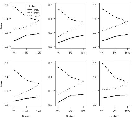
Our next step was to analyze the detection rate of the PE under both aberrant behaviors considered in this study. Figures 1 and 2 (for cheating and random
responding, respectively) display the detection rates found using a PE threshold value of .10; Table 7 summarizes the size of the effects found. The number of items
displaying aberrant behavior (k.aberr) had the largest effect on the detection rates in both settings. Interestingly, the detection rates were higher for a moderate value of k.aberr (= 5); both low and large values of k.aberr are associated with lower power. This finding is in line with results in St-Onge, Valois, Abdous, and Germain (2011), who showed that the detection rates of several person-fit statistics increase with aberrance rates only to some point, after which a decrease is to be expected. It was also observed that the cheating detection rates decreased with N.aberr. This can be understood by observing that the cheating behavior that we imputed led to sum-score differences (before versus after cheating imputation), which had a large impact on the original sum-scores (which were typically very low). In other words, the performance of PE seemed to decrease when the aberrance rate increased beyond moderate boundaries (St-Onge et al., 2011). The imputation of random responding behavior, on the other hand, was milder (the selected 0s were changes into 1s with a probability of .25). This introduced a more moderate rate of aberrant behavior in the data, and the PE statistic performed accordingly (for k.aberr = 3, 10): Its detection rate improved with N.aberr. The k.aberr = 5 in the random responding case was different because the PE’s detection rate decreased with N.aberr.
FIGURE 2. Random responding detection rate of PE for a number of items equal to 15 (top left), 16 (top middle), 17 (top right), 18 (bottom left), 19 (bottom middle), and 20 (bottom right).
TABLE 7
Effect of N.aberr, k.aberr, and length on detection rates for cheating and random responding
N.aberr k.aberr length Global Effect
Cheating ω2 = .09 ω2 = .22 ω2 = .03 R2 = .34 Random responding ω2 = .00 ω2 = .26 ω2 = .01 R2 = .27
Note.N.aberr = number of simulated test takers displaying aberrant behavior; k.aberr = number of items whose scores have been changed in order to display aberrant behavior; length = number of items in the dataset; global effect = fit of the regression model using main effects only.
Once more, the explanation resides in the balance that must exist between the performance of a person-fit statistic (PE in this study) and the level of aberrant rate in the data. When k.aberr = 5 the actual detection rate is larger than for the other values considered, but adding more and more “aberrant” test takers to the set did surpass some “breakpoint” of the PE statistic, which affected its performance for higher rates of aberrant test takers in the data.
In general, it can be concluded that the PE performed very well in the cheating case and moderately well in the random responding case. The PE statistic did not seem to be overly affected by violations of IIO or other model assumptions. Several factors, such as the number of test takers and items displaying aberrant behavior, must be taken into account when judging the performance of PE. Also, we stress two important ideas that should be taken into account when attempting to perform any person-fit analysis (using PE or any other statistic). We find it important to check whether the item response model of choice fits the data adequately (as we did) and to check how the performance
Asymptotic Distribution of the PE Statistic
One limitation of the PE statistic is that its computation requires a complete
enumeration of all response patterns with the same length and total-correct score as the response pattern under inspection. This task becomes demanding for numbers of items larger than, say, 20 on an average personal computer. Table 2 illustrates how quickly the total number of response vectors increases as the number of items increases. Depending on the number of items, it might be possible to circumvent the problem by using supercomputers. Nevertheless, it would be useful to approximate the exact distribution of the PE statistic through an asymptotic distribution for long tests. In
Appendix B we show the statistical derivation (based on previous work by van der Flier, 1982) that we used in an attempt to approximate the exact distribution of PE for large tests. We confirmed that this approximate distribution worked well only for a very limited range of situations (i.e., when all the p-values are very close to each other) for tests consisting of 20 items. Hence, it is still not clear how many items are required in order for the approximate distribution to be useful for long tests. Future research that can clarify this issue, or that possibly presents different distributional alternatives, is needed.
Discussion
In this report, we discussed a nonparametric statistic to detect misfitting item score patterns that is based on complete enumeration of all possible item score patterns. A big advantage of this method compared to existing methods is that practitioners can use the PE using a prespecified probability level. A drawback is that it can only be used for tests of moderate length due to the rapid increase of computational labor as the number of items increases. It is important to observe that the procedure used here does not guarantee that aberrant behavior did indeed take place whenever a flagging occurs. The PE, as is usually the case for interpreting person-fit statistics, can only provide an indication of the presence of aberrant behavior. The PE should not be used as
conclusive evidence that aberrant behavior did occur. Some follow-up strategies (e.g., interviewing the flagged test takers, interviewing the proctors, consulting the seating charts) could provide more substantive information.
In practice some items may not fit the IRT model. A researcher finds himself then in the vexing position of having to remove items because of inferior psychometric quality and keeping items in the scale because longer tests are better suited to detect person misfit (Meijer, Sijtsma, & Molenaar, 1995). There are good arguments, however, in favor of first investigating the scale quality of a set of items before conducting person-fit research. Inspecting the psychometric quality of the items and removing items with insufficient quality reduces the error component when we try to interpret misfitting response behavior. When an item cannot be described by an IRT model (e.g., because it correlates negatively with other items), or when an item has low discrimination (i.e., low Hi value), its score is a very unreliable indicator of the latent variable. Taking these
the proportion-correct scores and thus does not account for the discrimination of an item. Thus, it is important to check for items with low discriminating power, as we did.
Finally, in this study we discussed the PE for dichotomous items, which are often encountered in educational and intelligence testing. However, this procedure can be generalized to polytomous item scores, which will be a topic for future research.
References
Birnbaum, A. (1962). On the foundations of statistical inference. Journal of the American Statistical Association, 57(298), 269–306. doi: 10.1080/01621459.1962.10480660 Drasgow, F., Levine, M. V., & McLaughlin, M. E. (1991). Appropriateness measurement
for some multidimensional test batteries. Applied Psychological Measurement, 15(2), 171–191. doi:10.1177/014662169101500207
Embretson, S. E., & Reise, S. P. (2000). Item response theory for psychologists. Mahwah, NJ US: Lawrence Erlbaum Associates Publishers.
Emons, W. H. M. (2008). Nonparametric person-fit analysis of polytomous item scores. Applied Psychological Measurement, 32(3), 224–247.
doi:10.1177/0146621607302479
Evers, A., Sijtsma, K., Lucassen, W., & Meijer, R. R. (2010). The Dutch review process for evaluating the quality of psychological tests: History, procedure, and results.
International Journal of Testing, 10(4), 295–317. doi:10.1080/15305058.2010.518325 Ferrando, P. J. (2012). Assessing inconsistent responding in E and N measures: An
application of person-fit analysis in personality. Personality and Individual Differences, 52(6), 718–722. doi:10.1016/j.paid.2011.12.036
Geisinger, K. F. (2012). Worldwide test reviewing at the beginning of the twenty-first century. International Journal of Testing, 12(2), 103–107.
doi:10.1080/15305058.2011.651545
Guttman, L. (1944). A basis for scaling qualitative data. American Sociological Review, 9, 139–150. doi:10.2307/2086306
Guttman, L. (1950). The basis for scalogram analysis. In S. A. Stouffer et al. (Eds.), Measurement and precision (pp. 60–90). Princeton NJ: Princeton University Press. Hemker, B. T., Sijtsma, K., Molenaar, I. W., & Junker, B. W. (1997). Stochastic ordering
using the latent trait and the sum score in polytomous IRT models. Psychometrika, 62(3), 331–347. doi:10.1007/BF02294555
International Test Commission (2011). ITC guidelines for quality control in scoring, test analysis, and reporting of test scores. Retrieved from http://intestcom.org.
Karabatsos, G. (2003). Comparing the aberrant response detection performance of thirty-six person-fit statistics. Applied Measurement In Education, 16(4), 277–298. doi:10.1207/S15324818AME1604_2
Lee, P. M. (2004). Bayesian statistics: An introduction. West Sussex, UK: John Wiley & Sons Ltd.
Ligtvoet, R., van der Ark, L. A., te Marvelde, J. M., & Sijtsma, K. (2010). Investigating an invariant item ordering for polytomously scored items. Educational and Psychological Measurement, 70(4), 578–595. doi:10.1177/0013164409355697
Magis, D., Raîche, G., & Béland, S. (2012). A didactic presentation of Snijders’s lz* index of person fit with emphasis on response model selection and ability estimation. Journal of Educational and Behavioral Statistics, 37(1), 57–81.
doi:10.3102/1076998610396894
Meijer, R. R. (1994). The number of Guttman errors as a simple and powerful person-fit statistic. Applied Psychological Measurement, 18(4), 311–314.
doi:10.1177/014662169401800402
Meijer, R. R., & Egberink, I. J. L. (2012). Investigating invariant item ordering in
personality and clinical scales: Some empirical findings and a discussion. Educational and Psychological Measurement, 72(4), 589–607. doi:10.1177/0013164411429344 Meijer, R. R., Egberink, I. J. L., Emons, W. H. M., & Sijtsma, K. (2008). Detection and
validation of unscalable item score patterns using item response theory: An illustration with Harter’s self-perception profile for children. Journal of Personality Assessment, 90(3), 227–238. doi:10.1080/00223890701884921
Meijer, R. R., & Sijtsma, K. (1995). Detection of aberrant item score patterns: A review of recent developments. Applied Measurement in Education, 8(3), 261–272.
doi:10.1207/s15324818ame0803_5
Meijer, R. R., & Sijtsma, K. (2001). Methodology review: Evaluating person fit. Applied Psychological Measurement, 25(2), 107–135. doi:10.1177/01466210122031957 Meijer, R. R., Sijtsma, K., & Molenaar, I. W. (1995). Reliability estimation for single
dichotomous items based on Mokken’s IRT model. Applied Psychological Measurement, 19(4), 323–335. doi:10.1177/014662169501900402
Meijer, R. R., Tendeiro, J. N., & Wanders, R. B. K. (in press). The use of
nonparameteric IRT to explore data quality. Handbook of Item Response Theory Methods as Applied to Patient Reported Outcomes.
Mokken, R. J. (1971). A theory and procedure of scale analysis. Berlin, Germany: De Gruyter.
Mokken, R. J., & Lewis, C. (1982). A nonparameteric approach to the analysis of dichotomous item responses. Applied Psychological Measurement, 6(4), 417–430. doi:10.1177/014662168200600404
Molenaar, I. W., & Sijtsma, K. (2000). User’s manual MSP5 for windows. Groningen: IEC ProGAMMA.
R Development Core Team (2011). R: A language and environment for statistical computing. Vienna, Austria: R Foundation for Statistical Computing. Retrieved from
http://www.R-project.org/.
Sijtsma, K., & Junker, B. W. (1996). A survey of theory and methods of invariant item ordering. British Journal of Mathematical and Statistical Psychology, 49(1), 79–105. doi:10.1111/j.2044-8317.1996.tb01076.x
Sijtsma, K., & Meijer, R. R. (2001). The person response function as a tool in person-fit research. Psychometrika, 66(2), 191–207. doi:10.1007/BF02294835
Sijtsma, K., Meijer, R. R., & van der Ark, L. A. (2011). Mokken scale analysis as time goes by: An update for scaling practitioners. Personality and Individual Differences, 50(1), 31–37. doi:10.1016/j.paid.2010.08.016
Sijtsma, K., & Molenaar, I. W. (2002). Introduction to nonparametric item response theory. Thousand Oaks, CA: SAGE Publications, Inc.
Snijders, T. A. B. (2001). Asymptotic null distribution of person fit statistics with estimated person parameter. Psychometrika, 66(3), 331–342.
doi:10.1007/BF02294437
St-Onge, C., Valois, P., Abdous, B, & Germain, S. (2011). Accuracy of person-fit statistics: A Monte Carlo study of the influence of aberrance rates. Applied Psychological Measurement, 35(6), 419–432. doi:10.1177/0146621610391777 Tukey, J. W. (1977). Exploratory data analysis. Reading, MA: Addison-Wesley
Publishing Company.
van der Ark, L. A. (2007). Mokken scale analysis in R. Journal of Statistical Software, 20(11), 1–19.
van der Ark, L. A. (2012). New developments in Mokken scale analysis in R. Journal of Statistical Software, 48(5), 1–27.
van der Flier, H. (1982). Deviant response patterns and comparability of test scores. Journal of Cross-Cultural Psychology, 13(3), 267–298.
Appendix A: R Code for Computing PE
Function “uniqueperm2” (retrieved from
http://stackoverflow.com/questions/5671149/permute-all-unique-enumerations-of-a-vector-in-r) generates all unique permutations of a dichotomous vector x of size n. Function “PE” computes the PE for each person (= row) of the dataset “Data”.
uniqueperm2 <- function(x) { dat <- factor(x) N <- length(dat) n <- tabulate(dat) ng <- length(n) if(ng==1) return(x) a <- N-c(0,cumsum(n))[-(ng+1)]
foo <- lapply(1:ng, function(i) matrix(combn(a[i],n[i]),nrow=n[i])) out <- matrix(NA, nrow=N, ncol=prod(sapply(foo, ncol)))
xxx <- c(0,cumsum(sapply(foo, nrow))) xxx <- cbind(xxx[-length(xxx)]+1, xxx[-1]) miss <- matrix(1:N,ncol=1) for(i in seq_len(length(foo)-1)) { l1 <- foo[[i]] nn <- ncol(miss)
miss <- matrix(rep(miss, ncol(l1)), nrow=nrow(miss)) k <- (rep(0:(ncol(miss)-1), each=nrow(l1)))*nrow(miss) + l1[,rep(1:ncol(l1), each=nn)]
out[xxx[i,1]:xxx[i,2],] <- matrix(miss[k], ncol=ncol(miss)) miss <- matrix(miss[-k], ncol=ncol(miss))}
k <- length(foo)
out[xxx[k,1]:xxx[k,2],] <- miss
out <- out[rank(as.numeric(dat), ties="first"),] foo <- cbind(as.vector(out), as.vector(col(out))) out[foo] <- x
t(out)}
PE <- function(Data){ Nsubs <- dim(Data)[1]; Nitems <- dim(Data)[2];
if (Nitems > 20) {print("Number of items is > 20. Abort."); break}; Ps <- as.vector(apply(Data,2,sum) / Nsubs);
Qs <- 1-Ps;
possible.NC <- as.numeric(levels(factor(apply(Data,1,sum)))) PEvec.data <- rep(NA,Nsubs);
NC <- possible.NC[itms];
Data.NC <- uniqueperm2(c(rep(1,NC),rep(0,Nitems-NC)));
Nvecs.NC <- if (length(Data.NC)==Nitems){1} else {dim(Data.NC)[1]}; Pvec <- NULL; if (Nvecs.NC > 1){ for (i in 1:Nvecs.NC){ Pvec <- c(Pvec,prod(Ps^Data.NC[i,])*prod(Qs^(1-Data.NC[i,])))}} PEvec <- NULL; if (Nvecs.NC > 1){
for (i in 1:Nvecs.NC){PEvec <- c(PEvec,sum(Pvec[Pvec <= Pvec[i]])/sum(Pvec))}} else {PEvec <- c(1)}; suitable.subs <- which(apply(Data,1,sum) == NC); if (Nvecs.NC > 1){ for (i in 1:length(suitable.subs)){ sub=1;
while (sum(abs(Data.NC[sub,]-Data[suitable.subs[i],])) > 0 & sub <= Nvecs.NC){sub <- sub+1}
PEvec.data[suitable.subs[i]] <- PEvec[sub];}}
else {for (i in 1:length(suitable.subs)){PEvec.data[suitable.subs[i]] <- 1}}} PEvec.data;}
Appendix B: An Attempt to
Derive an Asymptotic Distribution of the PE Statistic
Consider the likelihood of response vector x (x1,x2,,xk) with total score X :
Lx = log(p(Xx)) =
k i i k i i i i p p p x 1 1 1 log 1 log =Vx C. (B-1)The likelihood of x is a sum of two terms: a random variable denoted Vx and a constant term that does not depend on x. If the number of items is sufficiently large (k 20) and if the set of p-values displays a “reasonable variance” (van der Flier, 1982, p. 295), then it can be shown that Vx (conditional on X) is asymptotically normally distributed with mean
k i i k i i i i i k i i i k i i i i p p p p p p p p p p 1 1 1 1 X ) 1 ( 1 log ) 1 ( 1 log (B-2) and variance
k i i i i i k i i i k i i i i i p p p p p p p p p p 1 2 1 2 1 2 ) 1 ( 1 log ) 1 ( 1 log ) 1 ( (B-3)(van der Flier, 1982, pp. 295–296). As a consequence, it can be concluded that Lx
(conditional on X) is asymptotically normally distributed with mean
k i i L p 1 ) 1 log( and variance L2 2 under the conditions previously stated. This result allows deriving an asymptotic distribution for p(Xx)exp(Lx) conditional on X :
L L p p P p P
0 0 0 log log ) exp(Lx Lx , (B-4)We considered using the right-side expression of Equation (B-4) as an
approximation for PE