Visualizing Changes of Hierarchical Data using Treemaps
Ying Tu and Han-Wei ShenAbstract—While the treemap is a popular method for visualizing hierarchical data, it is often difficult for users to track layout and attribute changes when the data evolve over time. When viewing the treemaps side by side or back and forth, there exist several problems that can prevent viewers from performing effective comparisons. Those problems include abrupt layout changes, a lack of prominent visual patterns to represent layouts, and a lack of direct contrast to highlight differences. In this paper, we present strategies to visualize changes of hierarchical data using treemaps. A new treemap layout algorithm is presented to reduce abrupt layout changes and produce consistent visual patterns. Techniques are proposed to effectively visualize the difference and contrast between two treemap snapshots in terms of the map items’ colors, sizes, and positions. Experimental data show that our algorithm can achieve a good balance in maintaining a treemap’s stability, continuity, readability, and average aspect ratio. A software tool is created to compare treemaps and generate the visualizations. User studies show that the users can better understand the changes in the hierarchy and layout, and more quickly notice the color and size differences using our method.
Index Terms—Treemap, tree comparison, visualize changes, treemap layout algorithm.
1 INTRODUCTION
The treemap is a popular method for visualizing hierarchical data. By dividing the display area into rectangles recursively according to the hierarchy structure and a user-selected data attribute, treemaps can ef-fectively display the overall hierarchy as well as the detailed attribute values from individual data entries. Since the treemap was first intro-duced [5] in 1991, data from many applications have been visualized with treemaps. Examples include file systems [5], sports [10], stock data [12], and social cyberspace data [7].
While the treemap has already been accepted as a powerful method for visualizing hierarchical data, there still exist additional visualiza-tion requirements yet to be addressed by treemaps. One of the needs is for users to visualize the difference when the data undergo changes. As a data set evolves over time, for example, the changes can range from major structure differences that affect the relationships among data en-tries, to subtle attribute value changes in individual data entries. How easily viewers can capture the changes in the data often determines how effective the visualization is to answer specific questions. Tak-ing file systems as an example, it is preferable for the treemaps to clearly reflect the overall changes in the directory structure as well as the changes of individual file attributes.
Effective visualization of changes in hierarchical data using treemaps is still an open challenge. The primary goal of our work for visualizing changes using treemaps is to compare treemaps which represent snapshots of data in different time points. Currently, the common approaches to comparing treemaps are to view them side by side or switch back and forth. But those approaches suffer from several common problems that can prevent viewers from performing effective data analysis:
• Abrupt layout changes: if small local changes in the data cause relatively large or global changes in the treemap layout, viewers are more likely to be overwhelmed by the differences and cannot easily identify the changes in the data.
• Lack of prominent visual patterns to represent the layout: with-out a prominent visual pattern, it is difficult for viewers to scan the map items in order and thus harder to track changes.
• Ying Tu is with the Computer Science and Engineering Department at the
Ohio State University, E-mail: [email protected].
• Han-Wei Shen is with the Computer Science and Engineering Department
at the Ohio State University, E-mail: [email protected]. Manuscript received 31 March 2007; accepted 1 August 2007; posted online 27 October 2007.
For information on obtaining reprints of this article, please send e-mail to: [email protected].
• Lack of direct contrast to highlight differences: if the attributes of the corresponding data entries are displayed separately in dif-ferent places with difdif-ferent contexts, viewers have to do indirect visual comparison, which creates difficulties in observing subtle differences.
In this paper, we take on this challenge and present strategies to visualize changes in hierarchical data using treemaps. To achieve our goal, we first propose a new treemap layout, thespiral layout, to reduce abrupt layout changes and generate a consistent visual pat-tern. Based on this representation, we propose the method ofcontrast treemapsto effectively compare two treemap snapshots and highlight the changes in one view.
The main idea of the spiral treemap is to use ‘spirals’ as the under-lying visual pattern to guide the placement of treemap items. In our spiral layout algorithm, items with the same parent in the tree are or-ganized along a spiral. By doing so, any two adjacent data entries in the hierarchy will remain adjacent in the layout, and the sibling data entries together form a consistent spiral pattern. The use of spirals reduces abrupt layout changes, so that neither the overall pattern nor the specific order of data entries will change drastically as the data continue evolving. In addition, map items that belong to different sub-trees can be easily distinguished as they are placed in different spirals. Moreover, our spiral layout algorithm provides a reasonably good as-pect ratio, which is necessary for us to display the contrast between data attributes in two treemaps. We evaluated the spiral treemap lay-out using the metrics proposed by Shneiderman and Wattenberg [2]. We also proposed two additional metrics to better measure the layout with respect to dynamic data. Experimental results show that the spiral treemap is spatially continuous, relatively stable and readable, and has adequately low aspect ratios.
Besides the spiral treemap layout, we propose acontrast treemap method for comparing treemaps. The main idea of the contrast treemap is to allow directcomparisons of the attributes in the cor-responding data entries at two time points. A contrast treemap is a treemap that encodes the information from two different snapshots of dynamically evolving data. Based on tree mapping techniques, cor-respondences between data entries can be formed automatically, and then a contrast treemap is built upon the union of both trees. By map-ping the corresponding items from two snapshots of data to a single item in the contrast treemap, we can use the item area to display the attributes from both snapshots and emphasize the difference in mul-tiple ways. Effectively, the contrast treemap eliminates the need for users to look back and forth between two separate items when com-paring their data values. As a result, differences become more explicit and easier to capture by viewers. A user study with statistical data of players in the National Basketball Association (NBA) shows that our Published 14 September 2007.
contrast treemap can better assist viewers in capturing and analyzing differences.
The rest of this paper is organized as follows: In Section 2, we briefly review the related work on treemap layouts and visualization techniques for tree comparison. In Section 3, we introduce the spiral treemap layout and compare it with other popular treemap algorithms. In Section 4, we present the contrast treemap and the techniques used for visualizing changes. Our user study is described in Section 5. Fi-nally, we summarize our work in Section 6.
2 RELATEDWORK
Tree Comparisons: Our visualization techniques are designed to
compare hierarchical data with treemaps. Using visualization to as-sist tree comparisons has been studied before. For example, Munzner et al.[8] compare phylogenetic trees. The focus of their comparison is on the tree structures. In this paper, we mainly focus on attributed trees, trees whose leaf nodes are associated with attributes. Our visu-alization not only highlights the structure differences of two trees, but also emphasizes the attribute and treemap layout changes.
Two previous works have compared trees with treemaps. One is the Univ. of Maryland’s Treemap 4.1 [6]. This software includes a slider control feature for multiple time series, a useful way to view treemaps at different time steps. This feature allows users to detect whether there are any changes to the treemaps, but it is not easy for them to analyze what exactly the changes are. Our visualizations are particularly designed for assisting change analysis.
Another work is the market mapapplication [12], which uses a treemap to show the rate of performance changes to popularly held stocks. The methods presented in this application are different from ours in two ways. First, we introduce shadings to indicate rates, an al-teration whose advantage will be explained in Section 4.2.3. Second, when displaying the change rates, we show hierarchical differences, a type of differences which is not handled in themarket map. In ad-dition, our visualization is a general solution which can help users analyze a variety of dynamic data types.
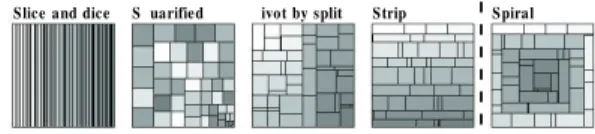
Slice and dice S uarified ivot by split Strip Spiral
Fig. 1. Examples of Layouts.
Treemap layout algorithms: A treemap layout algorithm is a
subdivision of rectangular areas representing internal tree nodes into smaller rectangles representing the children of the nodes. When the treemap was introduced [5], the slice-and-dice algorithm was the only layout. It uses parallel lines to divide the rectangle. Later, more treemap layout algorithms were proposed. The most well known algo-rithms are listed below with comments about their characteristics [9]. An example of each layout is shown in Figure 1. The intensity of the rectangles represents the order of the nodes in the tree.
• Slice-and-dice: Ordered, poor aspect ratios, best stability • Squarified: Unordered, best aspect ratios, medium stability • Pivot (or called “ordered”): Partially ordered, medium aspect
ra-tios, medium stability
• Strip: Ordered, medium aspect ratios, medium stability Recently, Viegenet al. [11] proposed variations to the squarified treemap. In the standard squarified algorithm the nodes are sorted by decreasing node size, and the strips are placed along the longest edge, either the left or bottom edges, of the rectangle. In the extended algorithm, the nodes can be sorted by increasing node size and the strips can be placed along the right and top edges. The variations produce different looks in terms of where the smallest and largest map items are placed.
Our spiral treemap layout generates a continuous and consistent vi-sual pattern, an advantage not possessed by many layout algorithms except the slice-and-dice. However, since the slice-and-dice can have
items of very poor aspect ratios, it is often not used. Our spiral lay-out has one thing in common with the extended squarified treemap: the strips can be placed along any edge in the rectangle. The biggest differences between these two layouts are the spatial continuity and the primary design goal. In a later section, we show that the spiral treemap performs well according to the metrics developed by Bed-erson, Shneiderman, and Wattenberg [2]. We also add several new metrics to analyze the layouts from additional aspects.
Content of treemap items: Typically treemap items are in a
uni-form color, which represents a value, but the inuni-formation represented by an item can actually be more expressive. For example in [1], each treemap item is occupied by an image, so the treemap can be used as an image browser. In this paper, we encode additional information while displaying the treemap items to show the contrast between two tree nodes’ data.
Furthermore, in order to highlight the spiral visual pattern, we use shading on the spiral treemap. Shading on treemaps was first intro-duced by van Wijk and Wetering [14]. Their goal of shading was to provide insight into the hierarchical structure, in particular the parent-child relationship, but the neighboring relationships were not partic-ularly emphasized. The original shading algorithm in the cushion treemaps cannot completely satisfy our need, thus we modify their algorithm to obtain the desired effects.
3 SPIRALTREEMAP
In this section, we describe how the spiral treemap was designed to be a continuous layout with a clear and consistent visual pattern. We also present an algorithm that creates the spiral layout with a good average aspect ratio to ensure the map items’ visibility, with an evaluation of the layout at the end.
3.1 Continuous Layouts
The design goal of our treemap layout is to avoid abrupt layout changes for dynamic data and also produce a clear and consistent vi-sual pattern, so that viewers can scan the items in order according to the pattern, effectively search for specific items, and keep track of the changes in the data. Among the existing treemap algorithms, the one that can most nearly meet the requirement of our goal while maintain-ing a good aspect ratio for the treemap items is the strip treemap. Strip treemaps place treemap items in a set of strips, which form a consis-tent visual pattern. While the algorithm can produce relatively stable layouts, it can occasionally show abrupt layout changes along with the changes of the attribute values. For example in Figure 2, a map item may shift from the end of one row to the beginning of the next row or vice versa. Essentially, the abrupt layout change is caused by spatial discontinuity.
Fig. 2. An example of the strip treemap’s spatial discontinuity. Because of size attribute changes, the item in green shifts from the end of the first row to the beginning of the second row. Its neighboring relationship with the blue item breaks, and a new neighboring relationship with the orange item is established.
Spatial discontinuity is the opposite concept of spatial continuity. By spatial continuity, we mean that for any two nodes in the tree that are next to each other in a given order, their corresponding map items are also neighbors in the treemap. Here we introduce the concepts ofadjacency arrowsandflow contoursto analyze the layouts’ spatial continuity.
Adjacency arrows are the building blocks of a flow contour. An adjacency arrowis a straight arrow from the center of a map itemMA to the center of another map itemMBif the node ofMA, A, in the tree is right before the node ofMB, B. Since A and B are adjacent tree nodes, the arrow indicates the adjacency information.
Aflow contourof an internal node is formed if all adjacency arrows among the node’s children are drawn on the treemap. The flow contour
starts from the first child’s map item, traverses through every child, and ends at the last child’s map item. Figure 3 shows an example of a flow contour. We can deduce the following property related to flow contours and spatial continuity: The flow contour of an internal node will go through the map item of every child of the node once and only once, and be free of intersections if and only if the treemap is spatially continuous, i.e. it holds spatial continuity. This property can be used to decide whether a treemap is spatially continuous. In addition, when a treemap layout algorithm guarantees to generate continuous treemaps, we say the layout of this algorithm is continuous.
(a) (b) (c)
Fig. 3. Tree nodes’ order and the flow contour. (a) shows the order among the tree nodes. (b) shows the adjacency arrows. The big pink flow in (c) is the flow contour.
3.2 Layouts with a Consistent Visual Pattern
When the flow contours of every treemap generated by a particular layout algorithm has a similar appearance, we say this layout has a consistent visual pattern. A consistent visual pattern can help viewers effectively scan the tree nodes in order, and hence makes it easier to create a visual mapping between two treemaps. An ideal visual pattern should also clearly reflect the hierarchies of the data, i.e., the parent-child relationship is clearly reflected in the patterns.
We use flow contours to aid the design of the treemap layout. The flow contour is used as a topological abstract of the treemap layout. Using flow contours, the problem of creating a visual pattern of a treemap layout can be reduced to the problem of shaping the flow con-tours. If the resulting flow contour is of a visually consistent pattern, so will be the layout. In fact, the concept of flow contours is similar to that of space-filling curves by Wattenberg [13]; the major differ-ence is that we want to use rectangular-shaped map items (internal or leaves) in the resulting treemap since rectangles make it easier to detect subtrees or branches. It is also easier to display additional con-tent/visualizations inside a rectangular area.
To find a flow contour pattern for our layout, we intend to use some-thing that we are familiar with. We propose to use spirals as the un-derlying flow contour pattern to guide the placement of treemap items. The flow contours extracted from a spiral layout are visually consis-tent even when the sizes of individual map items change. Take the spirals, (a) and (b) in Figure 4 for example: (a) is smaller and the dis-tance between the arcs shrinks as the spiral swirls in; (b) is larger and has a constant distance between adjacent parallel arcs. Although they are different, the visual pattern, which is a clockwise spiral shape, is clearly identical. Since we prefer rectangular-shaped map items, and want to make the best use of the area in the bounding rectangle, we adapt the classic spirals to be rectangular spirals, such as (c) in Figure 4.
(a) (b) (c) (d) Fig. 4. Spiral Examples and an S-Shape Example.
Of course, a spiral is not the only flow shape that possesses a con-sistent visual pattern. The s-shape flow is an alternative, such as (d) in Figure 4. An s-shape flow flips orientation between east and west. The angle of each direction change is 180 degree. The spiral flows produced by our algorithm will only make 90 degree turns at a time, which are easier to follow, comparatively.
3.3 Creating Spiral Layout
Like every other treemap layout algorithm, our spiral treemap is structed in a recursive manner. In essence, the resulting treemaps
con-tain nested spirals, where the children of each internal tree node form a spiral inside the rectangular space assigned to the node. Since our algorithm runs recursively for each internal node of the tree, in the fol-lowing, we describe our spiral layout algorithm only for a node and its children.
Given a list of map items, the key to form a spiral and occupy the entire given rectangular area is to subdivide the item list into segments, as shown in Figure 5, and lay out those segments in an iterative north-east-south-west spiral pattern.
1st Seg. 2nd Seg. 3rd Seg. 4th Seg. 5th Seg.
(a) (b) (c) (d) (e)
……
……
Fig. 5. Rectangular Spirals: In (a), the 1st segment fits in the north side of the given rectangle; in (b), the 2nd segment fits in the east side of the remainder of the given rectangle; in (c) and (d), the 3rd and 4th segment fit in the south and west; in (e), the 5th segment goes back to the north and is placed under the first 1st segment. When a segment fits into some place, its area does not change, but the width and height are adjusted. The alignment of items in a segment is decided according to the orientation of a segment.
A spiral layout is naturally continuous and has a consistent visual pattern, but the treemap items do not necessarily have good aspect ra-tios. Clearly, given some criteria, the optimal segment subdivisions to produce the lowest aspect ratio can be found by a brute-force method that exhausts all the combinations. However, it would be prohibitively expensive when a tree is deep and fat. When designing the spiral treemap layout algorithm, we are inspired by the strip treemap algo-rithm [2]. Strip treemaps work by placing the rectangular items one at a time into a horizontal (or vertical) strip of varying thicknesses, as in the example in Figure 1. If adding a new item to the current strip will decrease the average aspect ratio, the new item is added; otherwise, a new strip is started from the next row with the item. Since the strip layout algorithm uses the best local average aspect ratio as the condi-tion to finalize a strip, the average aspect ratio of all input items is well maintained.
To control the aspect ratio, we use a similar approach to the strip treemap algorithm. A segment in the spiral layout is like a strip in the strip layout, except that the orientation of the segment alternates in an east-south-west-north manner. The essence of the spiral algorithm is the following. Assuming a node hasnchild nodes,L1... Ln, in a given order to occupy the rectangle R, assigned to the node. We first scale the areas for the child nodes so that the total area will be equal to the area ofR. Then, we insert the map item for the first nodeL1to Rat the north (pointing to east). Since this is the only node inserted so far, it will occupy the entire width ofR. Because the area forL1is known, we can calculate its height and also calculate the aspect ratio. After this, the map item for the second nodeL2is inserted to the east ofL1’s. With the same principle, now with the total area ofL1and L2, and knowing that both of the nodes cover the entire width ofR, we can re-calculate the new height for the segment, as well as the new average aspect ratio. If the average aspect ratio increases as the result of adding this new item, we start a new segment which now points south using the rectangular space left under the north segment. We repeat this algorithm to insert all child nodes’ map items but alternate the orientations of the segments in the order of east, south, west, and north, and so on.
The last treemap in Figure 1 is generated by the above algorithm. If we compare this treemap with the strip treemap on its left, it can be seen that their average aspect ratios are similar. Later in this paper, we will study the spiral algorithm’s average aspect ratio, as well as continuity, stability and readability and compare it with other layout
algorithms in Section 3.5.
3.4 Spiral Visual Cues
As we said in Section 3.1, if viewers can detect flow contours, they can scan the items more easily along the order defined by the tree. To make the spiral patterns even easier to detect, we use shading as a vi-sual cue to highlight the neighboring relationships in the order given. Since a spiral can be seen as a set of connected segments in four differ-ent oridiffer-entations, detecting segmdiffer-ents is essdiffer-ential for iddiffer-entifying spirals. For this reason, we shade a segment as a metal tube to highlight its orientation and boundary. Figure 6 shows examples of shading the spirals.
Fig. 6. Shading for a Spiral. The left one shows the shading to high-light segments; the right one has additional shading for seams between items.
3.5 Analysis of Spiral Treemaps
To evaluate the effectiveness of the spiral treemap layout algorithm, we conducted experiments to compare it with the slice-and-dice, squari-fied, three different pivot layouts, and strip layout algorithms.
3.5.1 Metrics
To compare the treemap algorithms, in [2], theaverage aspect ratio,
average distance change, andreadabilitywere defined.
• Average aspect ratio. It is defined as the unweighted arithmetic average of the aspect ratios of all leaf-node rectangles. The ideal average aspect ratio would be 1.0, which would mean every item is a perfect square.
• Average distance change. It quantifies how much an item changes its position and size in terms of the Euclidean distance as data are updated.
• Readability. It quantifies how easy to visually scan a layout to find a particular item, based on how many times viewers’ eyes have to change scan direction when traversing a treemap layout in order.
To compare additional aspects of the treemaps, we define the fol-lowing new metrics.
• Continuity. Similar to readability, continuity also reflects how easy it is to visually scan a layout to find a particular item. It quantifies how many times viewers’ scanning flow is interrupted when the next item is not a neighbor of the current item. Assume
a parent node containsxchild nodes, then there arex−1 pairs
of adjacent tree node siblings. We count the number of pairs of adjacent tree node siblings that are neighbors in the layout, say
y, so x−y1 is the value of this layout’s continuity. If the layout
is continuous, the scanning flow is free of interruption, so the continuity is the best, which is 1.0. We define the continuity for hierarchical layouts similar to the way readability was defined in [2]: the average of the continuity of the leaf-node layouts, weighted by the number of nodes contained in the tree.
• Variance of distance changes. This variance is a supplement to the average distance change. If the average distance change is low, but the variance is high, it means that although most items do not move much, some items move by large distances, which would cause abrupt layout changes.
3.5.2 Evaluation
We measured the effectiveness of treemap layouts using the experi-mental methods proposed in [2]. The experiment consisted of a
se-quence ofMonte Carlo trials to simulate temporally updated data.
The authors [2] provide a package of implementations of multiple lay-out algorithms and their evaluation methods. Based on their code, we added our spiral algorithm and metrics we defined to compare the spi-ral layout algorithm with others.
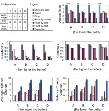
We performed experiments on multiple types of hierarchies to cover different cases. In our experiments, layouts were created for bounding rectangles of various aspect ratios, such as 1:1, 1:2, 2:1, and we also varied the tree breadth and depth. Due to limited space, we only show four representative configurations, as described in Figure 7. Other re-sults not shown in this paper displayed similar trend. For each experi-ment we ran 50 trials of 50 steps each.
The performance comparison of different treemap layouts is shown in Figure 7. Since our spiral layout is most similar to the strip layout,
we mainly focus on the trade-offs between them. Theaspect ratioof
the spiral layout is average: much smaller than the slice-and-dice lay-out, noticeably larger than the squarified laylay-out, similar to the rest. In
terms ofreadability, the spiral layout is a little worse than the strip
layout. But this is complemented by the perfectcontinuity, which is
important for tracking map items for treemap comparison. The
stabil-ity of the layout is mainly reflected byaverage distance change, for
which the spiral layout is better than the strip layout in most cases, except for the case where the aspect ratio is large. That is expected be-cause in that case, the strip layout has fewer rows and thus has fewer turns. But in the case where a small aspect ratio is used, the spiral layout is noticeably better. In real cases with a multi-level hierarchy, a wide range of aspect ratios will be used, and thus the spiral layout can achieve much lower average distance change, as shown in the
con-figurationD. In addition, thedistance change variationfor the spiral
layout is also significantly better than the strip layout. It means when a change happens, the positions of items in the spiral layout tend to change smoothly following the spiral pattern, which is less likely to introduce abrupt layout changes to confuse viewers.
Slice-and-dice Spiral Strip Pivot-by-middle Pivot-by-size Pivot-by-split Squarified Configurations: Width: Height Legend: Tree Breadth Tree Depth 1:1 A B C D 2:1 1:2 1:1 50 50 50 20 1 1 1 3 0 1 2 3 4 5 A B C D
(the lower the better)
Aspect Ratio 145 291 72 59 0 0.2 0.4 0.6 0.8 1 1.2 A B C D
(the higher the better)
Readability 0 0.2 0.4 0.6 0.8 1 1.2 A B C D
(the higher the better)
Continuity 0 5 10 15 20 A B C D
(the lower the better)
Average Distance Change 0 0.1 0.2 0.3 0.4 A B C D
(the lower the better)
Distance Change
Variation
Fig. 7. Performance of Multiple Treemap Layout Algorithms
In summary, our spiral layout is a well-rounded layout algorithm in general and especially suitable for treemap comparisons given its continuous and consistent visual pattern.
4 VISUALIZECHANGES/CONTRAST ONTREEMAPS
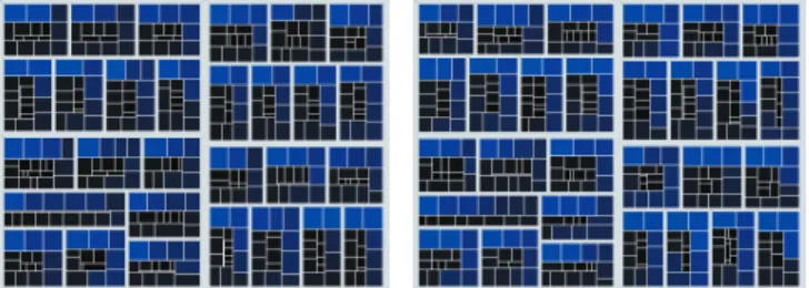
In this section, we introduce the concept ofcontrast treemaps. Un-like “spiral” in thespiral treemapand “strip” in the strip treemap, here the adjective “contrast” does not refer to a layout algorithm, but describes a treemap whose map items’ content incorporates informa-tion and highlights the contrast for comparing two treemaps. Exam-ples of treemap comparisons presented in this section are generated for the hierarchies using the online NBA statistics based on conferences, divisions, teams, and players1. In the example shown in Figure 8, the left treemap is for the 2002-2003 season and the right for 2003-2004 season. Both treemaps use “minutes/game” for thesize attribute, whose value determines a map item’s area, and “points/game” for the color attribute. As for the color encoding, blue means a large value of “points/game”, and black means a small value of “points/game”. Hereafter we will call the two compared treemaps as TM1 and TM2. The size and color changes reflect the changes of player performance; The hierarchical changes reflect the personnel changes, for example, new players, transferred players, and players who are missing from the second season.
Fig. 8. Two treemaps created from the NBA statistics of the 2002-2003 (left) and 2003-2004 (right) seasons.
4.1 Tree Mapping and Union Trees
Previously, a treemap was derived from a single tree, however, the contrast treemap is designed to show two trees’ information. Thus we defineunion treesto incorporate two trees into a single tree, and the contrast treemap is derived from the union tree.
Constructing a union tree of two trees is based on the assumption that the two trees can be mapped, so that any node in one tree has a counterpart in the other tree, otherwise it is assumed that this node is deleted from or inserted to the other tree.
1 2 3 4 4 C 1 2 3 3 4 1 2 4 5 5 A B D E A B D C F G E A B D D C C A B F G (a) (b) (c) Fig. 9. (c) is the union tree of (a) and (b).
We illustrate union trees in Figure 9. (a) and (b) are the trees to be compared, denoted asT1andT2; internal and leaf nodes are rep-resented as circles and squares; leaf nodes fromT1andT2are in grey and yellow respectively. The hierarchical changes fromT1 toT2are: the leaf node E ofT1is deleted; the internal node 4 ofT1is moved to be a child ofT2’s root; the internal node 5 is inserted with two children F and G to be under the node 3. (c) is the union tree of (a) and (b), denoted asTunion. The leaf nodes ofTunionare represented by trian-gles, with two squares, or one square and one diamond. The squares represent the node attribute information fromT1andT2, so a node in
Tunioncan access the attribute values ofT1andT2. If a node does not
exist inT1orT2, the copy of this node’s information inTunionis null and represented as a diamond.
1http://www.usatoday.com/sports/basketball/nba/statistics/archive.htm
Tree mapping relies on the tree mapping algorithms. In fact, com-paring tree structures and constructing the mapping is a research area being actively studied. Different types of trees need different tech-niques to map. The typical hierarchies that are proper to visualize with treemaps are rooted, labeled trees. Bille [3] surveyed the problem of comparing labeled trees based on simple local operations of delet-ing, insertdelet-ing, and relabeling nodes. S. Chawatheet al. [4] proposed algorithms based on more operations including moving and copying nodes. In case there is no obvious mapping between two hierarchi-cal data, mapping snapshots of a time-evolving hierarchy can be done using those algorithms.
For our case study of the NBA statistics, we assumed that the nodes in the hierarchy have unique keys, which are the names of the players. Mapping can be done by comparing keys, so a node withKeyiin one hierarchy and a node with the same key in the other hierarchy can be easily matched.
Size attribute of a contrast treemap:Like a regular treemap, any attribute can be used as the size attribute for a contrast treemap. Since an item of a contrast treemap can have two values for the attribute, one value from each treemap, there are several options to assign size to items. Assuming the values of the size attribute fromT1andT2for an item areS1andS2, for example: If we useS1, the layout will look exactly like the treemap ofT1; If we useS2, the layout will look like T2; We can also use the sum, max, or min ofS1andS2, or use an equal value for each item.
Layout of a contrast treemap:Although we can use any treemap layout algorithm for the contrast treemaps, the layouts with good as-pect ratio, stability and a clearly visual pattern are preferred, which has been reasoned in Section 3. So our examples all use the spiral layout. 4.2 Contrast Treemap Content Design
In the contrast treemap, we focus on using color-encoding of the leaf nodes’ map items to display changes, since most of the rectangular space is allocated to them. As will be seen in the examples, hierarchi-cal changes in the leaf nodes can be clearly seen by color highlights. Although we do not explicitly highlight the internal nodes’ structure changes, these changes can be implicitly inferred by their descending leaf nodes’ map items.
4.2.1 Two-Corner Contrast Treemap
In this section we introduce a scheme called thetwo-corner contrast treemap, to compare the attribute values of a map item from the two treemaps. A two-corner contrast treemap color-encodes the value con-trast in the treemap items to highlight the differences. Assuming the attribute to be compared isAk, the basic idea is to useAkasTunion’s color attribute, and for each map item, we assign the color of TM1’s value to the upper-left corner of the map item, and the color of TM2’s value to the lower-right corner, and blend the colors across the item’s area. If the attribute value of TM1 or TM2 is null, a diamond in the union tree, the whole item can be in the other treemap’s color; or a default color can be assigned for the absent nodes.
In Figure 10, we use five images to show some variations of the basic item content design in terms of how and where two colors are blended. The color from TM1 is green, and the color from TM2 is yellow. In (a), two colors are blended across the entire rectangle. Al-though it has a smoother color transition, it may be difficult for viewers to compare the original two colors to see the value difference. In (b), each color takes half of the space, but the contrast may be too strong to be visually pleasing when looking at the entire treemap. In (c), the two colors are smoothly blended by an intermediate band along the diagonal, so it looks more pleasing than (b). In (d) the attribute values from TM1 and TM2 are also encoded by the area occupancy, i.e. the space taken by each color is also determined by the attribute values: the larger the attribute value is, the more space its color occupies in the item. If desired, we can use the area occupancy to encode another attribute to accompany the color separation. In (e), the effects of (c) and (d) are combined.
The contrast treemap in Figure 11 compares TM1 and TM2 in Fig-ure 8. The size and color attributes are the same as in FigFig-ure 8. We use
the size attribute values of TM2 to decide the contrast treemap’s item sizes, so the players missing in the second season will not be seen. The layout looks slightly different from TM2 in Figure 8, because some space is taken by the abbreviated labels. The top-left corner is used to show the information of TM1 (02-03), and the bottom-right corner is for TM2 (03-04).
(a) (b) (c ) (d) (e)
Fig. 10. Design of the Contrast Treemap - Two Corners
The colors are blended like (e) in Figure 10. For an item, if both corners are in the blue to black range, the player was in the same team for both seasons. If the color for the 02-03 season is pine green, it means the player transferred to this team in the second season. If the color for the 02-03 season is dark yellow, the player joined the NBA in the second season. If the player played in the 02-03 season, no matter if he changed teams or not, the area occupancy of the map item is also encoded by “points/game”. We can compare the color or area to know in which season a player scored more points per game. Examples: (all example items in treemaps are surrounded with bright green circles)
• “Mc” in the Orlando Magic (Tracy McGrady) performed equally well in both season.
• “Red” in the Milwaukee Bucks (Michael Redd) performed bet-ter in the second season. Actually, the value of “points/game” increased from 15.1 to 21.7.
• There are two “Jack”s that transferred to the Houston Rockets, who are Mark Jackson and Jim Jackson. Mark’s 03-04 color is darker than Jim’s, so we know Jim was better. We can also see that, after they transferred to another team, Jim got better but Mark was not so lucky.
• Most of the new players did not get high “points/game”, so their color was dark, but “Ant” in the Denver Nuggets (Carmelo An-thony) and “Jam” in the Cleveland Cavaliers (LeBron James) were exceptions. Their colors are bright. Both of them received about 21 points/game in the 03-04 season.
Fig. 11. An Example of the Contrast Treemap - Two Corners 4.2.2 Texture Contrast Treemap
Besides the attribute value changes, sometimes it is necessary to com-pare the layouts between two treemaps to see where the major changes take place. The layout change includes changes in the map items’ width, height, position, and neighbors.
To achieve this goal, we can select an image as the background texture for the first treemap TM1. The positions of the treemap item
corners are normalized to [0,1] in each dimension and used as the tex-ture coordinates. When TM1 changes to TM2, some map item’s size and location may change but we keep the same texture coordinates for the item’s corners from TM1 and re-draw the treemap items accord-ing to TM2’s new layout. Since there are layout differences between TM1 and TM2, the input texture will be distorted and some portions of the texture will get displaced. Based on how the texture has changed, viewers can perceive the information about the layout changes.
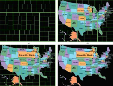
Figure 12 shows an example of this technique. Because there are a lot of and various changes between TM1 and TM2 of the NBA data, in order to better explain this technique, we simplify the scenario, using an arbitrary treemap to be TM1, and get TM2 by enlarging the size of an item in TM1 by 3 times. (a) is a typical treemap. In (b), an US map is selected to be the background image and mapped to (a). In (c), the treemap layout is changed from (b), where the size of an item aroundSouth Dakotais increased a lot. We removed the frame lines on (c), to result in (d). By observing (c) or (d), we know some large layout changes happened aroundSouth Dakota, minor layout changes happened aroundNorth CarolinaandSouth Carolina, and other parts do not have much change. To make use of this method, users can choose any background image that they are familiar with.
It is noteworthy that how much a layout changes does not always reflect how much item sizes or tree hierarchies change. For a unsta-ble layout, such as the squarified treemap, viewers cannot expect the extent of layout change to be proportional to that of the size or hier-archy changes. For relatively stable layouts, such as the spiral layout and slice-and-dice layout, viewers are able to see the extent of changes from the texture alteration.
(a) (b )
(c) (d ) Fig. 12. An Example of the Contrast Treemap - Texture Image
4.2.3 Ratio Contrast Treemap
When comparing the attribute values between two treemaps, some-times it is useful to know how much the value of a node from one tree is greater than, equal to, or less than the value of its corresponding node in the other tree. This can be done by calculating the ratio be-tween the two values and showing how the ratio compares to 1. To display this information in the contrast treemap, users can pick three base colors:low color,neutral color, andhigh color. Assuming the ratio is R, when R is less than, equal to, or greater than 1, the contrast treemap item is assigned thelow color,neutral color, orhigh color, respectively.
To further display the value of this ratio, colors, various saturation, brightness, and shading can be utilized, as shown in Figure 13 (a), (b) and (c). Yellow and green are set to be thehighandlow color, but differentneutral colorsare used. Given the color table, viewers can determine whether an attribute value increases or decreases, and also what the ratio is.
(a) (b) (c)
Fig. 13. Design of the Contrast Treemap - Ratio
In (a), shading is used to indicate the ratio. The principle is that the farther the ratio is away from 1, the sharper the contrast becomes, and the smaller the bright spot in the item will become. One advantage of using shading is that items with sharper shading contrast can attract viewers’ attention, which in this case, means the value difference is larger. Another advantage is that more base colors can be used to represent other information.
Figure 14 is an example of the Ratio Contrast Treemap. The layout of this treemap is the same as the treemap in Figure 11. It displays the ratios of the players’ two seasons “points per game”. Some players’ values were not high, but the ratio may be high. If the goal is to find some potential star players, this treemap might help. Red and pink are the high colors for untransferred and transferred players respec-tively. Green and lighter green are the low colors for untransferred and transferred players, respectively. New players are in dark yellow. Pine green is the neutral color. We can observe that, for example, the map items of “Mur” in the Seattle SuperSonics (Ronald Murray) and “Arr” in the Utah Jazz (Carlos Arroyo) have the sharpest red shading. The ratios were very high, which were121..94and 122..86 respectively.
Fig. 14. An Example of the Contrast Treemap - Ratio 4.2.4 Multi-Attribute Contrast Treemap
Sometimes viewers may want to compare more than two attributes between the data snapshots. In this case, since single color and size encoding is not sufficient, we design a method to show the contrast of multiple attributes by vertically dividing the area of an treemap item into multiple sub-areas. Each sub-area is used to represent one at-tribute and is horizontally divided into top and bottom halves in pro-portion to the value ratios of the attribute in the two trees. All top halves are in one color and all bottom halves are in a second color. Here, the value differences are not encoded by the gradient colors, but by the ratios of the heights of the top and bottom halves.
(a) (b) (c ) (d) Fig. 15. Design of the Contrast Treemap - Multi-Attributes
Figure 15 shows map item examples, where more than ten attributes are encoded, and a ragged line emerges, separating the top and bottom areas. The green color area is for data at the time point of TM1, and the cyan area is for TM2. In (a), we can see two attributes with dif-ferent values. In the case that a node is deleted from or inserted to TM2, then there is only one color in the whole item since there are no corresponding values available to divide the items into two halves, so the full green item (c) stands for a tree node being deleted, and the full cyan item (d) stands for a tree node being inserted. In this way, we can visualize the changes of the tree structure as well.
Figure 16 is an example. Every team’s rectangle contains all players that played in the team over the selected years and we let the size value for every player be equal. All the attributes were encoded. Cyan is for the 02-03 season, and yellow is for another season. Pine green is the background color. If a player was in one team for two seasons, the color pattern is cyan over yellow. If a player transferred from Team A to Team B, in A’s rectangle, the player’s color is cyan over pine green, and in B’s rectangle, the player’s color is pine green over yellow. If a player only played for one season, the whole item is colored by that season’s color. We can see that some players’ performance changed a lot from one season to the next. For example, for “Pipp” (Scottie Pippen), who transferred to the Chicago Bulls from the Portland Trail Blazers, the data show that he did not get as high statistical numbers in the Bulls as he did in the Trail Blazers.
Fig. 16. An Example of the Contrast Treemap - Multi-Attributes
5 USERSTUDY
To evaluate the contrast treemap, a user study based on the NBA statis-tics data set, described in Section 4, was conducted.
We performed the user study with 12 subjects. All the subjects were students majoring in computer science and engineering. They used computers for at least 7 hours daily. 25% were female and 75% were male. 17% were familiar with the NBA teams and players; 33% knew a little and 50% were unfamiliar. 42% did not know about treemaps before; 33% knew a little about treemaps; 25% knew treemaps well and had experience using treemaps to visualize data. For the subjects who did not have the knowledge of treemaps, a short tutorial was given before the experiments. The basic idea of the contrast treemaps were introduced to all subjects. The user study consisted of five sections of questions, explained below.
In the first section, the subjects looked at 3 treemaps, among which two were individual treemaps derived from each of the seasons, and the other was a two-corner contrast treemap that combined information from both seasons.
The contrast treemap’s color and size attributes are the same as in Figure 11, but the size value of an item is the sum of the size value in TM1 and TM2. Inserted, deleted, and moved items were highlighted with different colors.
The subjects were given 6 players’ names and teams for the 02-03 season. They were asked to find the players’ teams in the 03-04 season. The time for the search of each player was recorded. Among the 6 players, 2 stayed in the same team in the 03-04 season, 2 transferred, and 2 retired. The subjects were told that a player might not be in the treemap of the 03-04 season, hence they could give up if they could not find the player and believed he retired.
The test results collected from the case where the subjects looked at the two individual treemaps and searched for the players show that: 1) If the player stayed, the subjects almost spent no time finding the player’s team in the second year. 2) If he transferred, subjects gave up in 29% of cases. The average time to give up was 0.9 minute. For the cases of successfully locating a transferred player, the subject spent one minute on average. Considering two subjects gave up immedi-ately, i.e. they refused to search, it is not too surprising that the time to give up was shorter. 3) If the player left the NBA, the average time to give up was 1.5 minutes.
The test results from the case where the subjects looked at the con-trast treemap shows that all subjects spent no time searching for the missing players, and the giving up rate of searching for the transferred players dropped from 29% to 4%. That is because the contrast treemap highlighted the transferred, new, and missing players, thus the sub-jects could directly answer the questions when they saw the player was highlighted as a missing player; and when they were searching for the transferred players, they believed they could find the player so they did not give up easily. To search for the transferred players, excluding the single giving up case, the time spent on the contrast treemap was slightly less than one minute; the result that the time spent was shorter may be because the searching range was narrowed down to the players highlighted as “transferred”. We use this test to prove our assumption that searching can take a long time, and visual cues can help viewers avoid blindly searching.
In the second section, the subjects looked at the 3 treemaps used in the previous section. Three players and their teams were given, the subjects were asked to compare the performance of each player between both seasons from the individual treemaps. Then the subjects looked at the contrast treemap to answer the same question. 42% of the subjects were not sure about the color difference for at least one player from the two treemaps, but all subjects gave the correct answers from the contrast treemap. The subjects all stated that making comparisons in the contrast treemap was easier and faster than comparing the colors of items from two separate treemaps side by side.
In the third section, three players and their teams were given, and the subjects were asked to rank the ratios of performance changes for the players by looking at the per-season treemaps and a ratio contrast treemap. When looking at the per-season treemaps, most subjects re-verted colors to values according to the given color scale, calculated the rates and ranked them. 30% of the answers were wrong. When looking at the ratio contrast treemap, they quickly decided the rank, and only 11% of the answers were wrong. The result shows that com-paring subtle color differences for estimating ratio is difficult. The ratio contrast treemap can help viewers since the ratio itself has been converted to color.
In the fourth section, two distorted background contrast treemaps with their original background treemaps were shown to the subjects. The question asked was whether the subjects would like to use a map item’s texture to search for the item and whether the subjects thought the texture helped them find items that had big changes. 83% subjects stated that the texture was helpful and they liked searching textures. 17% subjects did not agree, because they preferred to match labels instead of images.
In the fifth section, a multi-attribute contrast treemap was shown. Given 2 players, the subjects were asked to compare the performance of each player and decide whether they performed better in the second season. All subjects gave the correct answers. They were also asked what they could see from the treemap; the options were how a player’s performance differed, whether a player changed teams, and whether a player was new or retired in the 03-04 season. All subjects believed that all the questions could be answered by looking at this treemap, as
Figure 16.
The user study results showed that incorporating two trees’ or two treemaps’ information to one contrast treemap can help users per-form data comparisons more effectively, and our design is effective to achieve the goals.
6 CONCLUSIONS ANDFUTUREWORK
In this paper, we introduced a new spiral treemap layout and pre-sented several techniques to visualize changes of hierarchical data us-ing treemaps. Experimental results show that our spiral layout is able to provide good continuity, stability, readability, and adequately low aspect ratio so that it is suitable for visually comparing evolving data. To highlight the changes, we proposed the contrast treemap, a novel approach to directly compare attributes from two snapshots of hier-archical data in one treemap. Along with the spiral treemap layout, our design overcomes three main challenges in comparing hierarchical data using treemaps: a) abrupt layout changes, b) a lack of prominent visual patterns to represent the layout, and c) a lack of direct contrast to highlight differences. We have developed a software tool based on our design to compare treemaps and generate visualizations. A compre-hensive user study has been conducted with statistical data of players in the NBA. The test results suggested that our contrast treemap can better assist viewers to compare data and analyze differences.
There are several directions for future research. First, we will de-velop efficient and optimized algorithms to cut segments for a spiral to produce better stability and average aspect ratio. Second, we will ex-periment different continuous and visually consistent layouts besides spirals. Third, we will continue to enhance the contrast treemap to express more channels of information.
ACKNOWLEDGEMENTS
This work is supported by NSF ITR Grant ACI-0325934, NSF RI Grant CNS-0403342, NSF Career Award CCF-0346883, and DOE SciDAC grant DE-FC02-06ER25779.
REFERENCES
[1] B. B. Bederson. Photomesa: a zoomable image browser using quantum
treemaps and bubblemaps. InACM symposium on User interface
soft-ware and technology (UIST ’01), 2001.
[2] M. W. Benjamin B. Bederson, Ben Shneiderman. Ordered and quantum
treemaps: Making effective use of 2d space to display hierarchies.ACM
Transactions on Graphics (TOG), 21(4), October 2002.
[3] P. Bille. A Survey on Tree Edit Distance and Related Problems. Theor.
Comput. Sci., 2005.
[4] S. Chawathe and H. Garcia-Molina. Meaningful change detection in
structured data. InACM SIGMOD International Conference on
Man-agement of Data, 1997.
[5] B. Johnson and B. Shneiderman. Tree-maps: a space-filling approach to
the visualization ofhierarchical information structures. InIEEE
Confer-ence on Visualization, 1991.
[6] H.-C. I. Lab. Treemap 4.1. http://www.cs.umd.edu/hcil/treemap.
[7] Miscosoft, http://netscan.research.microsoft.com/treemap/.
Pre-Rendered Tree Map Views of All Usenet and microsoft.public.
[8] T. Munzner, F. Guimbretiere, S. Tasiran, L. Zhang, and Y. Zhou. Treejux-taposer: scalable tree comparison using focus+context with guaranteed
visibility. InACM SIGGRAPH, 2003.
[9] B. Shneiderman. Treemaps for space-constrained visualization of hierar-chies. http://www.cs.umd.edu/hcil/treemap-history/index.shtml. [10] D. Turo. Hierarchical visualization with treemaps: making sense of pro
basketball data. InCHI ’94: Conference companion on Human factors in
computing systems, 1994.
[11] R. Vliegen and E.-J. van der Linden. Visualizing business data with
generalized treemaps.IEEE Transaction on Visualization and Computer
Graphics, 12(5), 2006.
[12] M. Wattenberg. http://www.smartmoney.com/marketmap.
[13] M. Wattenberg. A note on space-filling visualizations and space-filling
curves. InINFOVIS ’05: Proceedings of the Proceedings of the 2005
IEEE Symposium on Information Visualization, 2005.
[14] J. J. V. Wijk and H. van de Wetering. Cushion treemaps: Visualization of
hierarchical information. InINFOVIS ’99: Proceedings of the 1999 IEEE