Multistatic Passive Weather Radar

(1)

UNIVERSITY OF OKLAHOMA GRADUATE COLLEGE

MULTISTATIC PASSIVE WEATHER RADAR

A DISSERTATION

SUBMITTED TO THE GRADUATE FACULTY in partial fulfillment of the requirements for the

Degree of DOCTOR OF PHILOSOPHY By ANDREW BYRD Norman, Oklahoma 2020

(2)

MULTISTATIC PASSIVE WEATHER RADAR

A DISSERTATION APPROVED FOR THE

SCHOOL OF ELECTRICAL AND COMPUTER ENGINEERING

BY THE COMMITTEE CONSISTING OF

Dr. Robert Palmer, Chair

Dr. Caleb Fulton, Co-Chair

Dr. Nathan Goodman

Dr. Pierre Kirstetter

Dr. Alan Shapiro

(3)

(4)

For my wife, Suzy. I can’t imagine beginning this next great adventure with anyone but you.

(5)

Acknowledgments

I have to begin by thanking Robert Palmer and Caleb Fulton, who have been my advisors, my coauthors on the two journal papers that form the cornerstone of this dissertation, and my friends. Dr. Palmer extended my initial offer to work at the ARRC and has, since then, set an almost implausibly high standard for leadership. It is a very rare advisor or manager who may be so confidently depended upon for advocacy and invaluable insight (both technical and otherwise) by those who work for him. Dr. Fulton is a model of astonishing depth and breadth of technical brilliance, but also of how to take genuine joy in the work of engineering. I think most people at the ARRC have a great love for their work, but Dr. Fulton’s is so incandescent that it leaves you little choice but to have fun. Working for and with these two has truly been a privilege.

I also owe a tremendous debt to the family that has supported me through this journey. My mother, Janet, has helped to support me in every way possible through the years, and no thanks I give her will ever be sufficient. I am extremely grateful for my wife, Suzy, who has been incredibly loving and patient throughout this process. Suzy’s family, Fernando, Lupe, and Sylvia have also been wonderfully supportive and welcoming. They have truly given me a home in Oklahoma (quite literally in these last months).

Finally, there are some necessary acknowledgments specific to the work de-tailed in Chapters 3-5. I wish to extend special thanks to ARRC staff engineer Cody Piersall for his work on the radar control software, and to the administration and facilities staff at OUHSC (particularly Stuart Hall and Dustin Bozarth) for their extraordinary level of cooperation. Thanks to the administration and engineers at the Radar Operations Center (particularly Adam Heck, Steven Smith, and Terrance Clark) for their help in understanding the finer details of WSR-88D operations.

(6)

Thanks also to Alan Shapiro for his excellent suggestion of using the KTLX radial velocity comparison to validate the system and to David Bodine for several use-ful discussions of multistatic radar applications, as well furnishing the numerical weather prediction data used in the simulations for Chapter 5, and, in cooperation with Clarice Dyson, for operating the passive radars to collect the scattered con-vection observations in Chapter 4. Finally, thanks to Dusan Zrni´c for some helpful discussion and references regarding sidelobe whitening.

This work was supported by the National Severe Storms Laboratory through cooperative agreement NA15OAR4320115.

(7)

IEEE Copyright Notice

The contents of two journal papers (for which I was the first author) were reused substantially in Chapters 3-6 of this work. Chapters 3-4 are composed primarily of material drawn from [1] (©2019 IEEE). Chapter 5 is composed primarily of mate-rial from [2] (under review, IEEE). Chapter 6 contains substantial reprinted matemate-rial from [1] and [2]. There are additional figures, datasets, and explanations added to the material present in these papers. Some figures may appear slightly different from the corresponding figures in these works due to updates and improvements to the processing software. The paper structure has also been rearranged to accomo-date the dissertation format. However, these changes are not substantial enough to distinguish these chapters as new works independent from these papers.

(8)

List of Figures

2.1 The fundamental geometry of a bistatic radar observation includ-ing the transmitter rangeRT, receiver rangeRR, baseline lengthL,

and bistatic angleβ. The arrows indicate the direction of radiation propagation along each path. . . 14 2.2 An example of the transmitter and receiver locations as the focii

of an ellipse of constant range (shown in purple). This ellipse is a cross-section of the three-dimensional constant-range ellipsoid along the bistatic plane. For a scatterer located at any point on this ellipse, the bistatic rangeRB =RT+RRwill be constant. . . 17

2.3 The range and beamwidth boundaries that form a resolution vol-ume in a typical bistatic weather radar. The concentric ellipses cor-respond to constant bistatic range ellipses. The translucent cones represent the main beam widths of the transmitter and receiver. The resolution volume formed by the intersection of the transmit beam with the ellipses is highlighted by a black dashed line. . . 18 2.4 Example of a degenerate resolution volume geometry in which the

near bistatic range boundary is defined by the system baseline and the far bistatic range volume does not come into play, as the exterior volume edges are defined by the transmit and receive beampatterns. 22

(12)

2.5 Diagram of the geometric quantities used to calculate Cartesian scatterer coordinates in (2.12)-(2.14). . . 23 2.6 Echo localization through multilateration in a network consisting

of a single transmitter and three receivers. The purple ellipses rep-resent isorange contours corresponding to detection of the actual scatterer by each receiver. If only two receivers are used, there will be two candidate detection locations where the isorange contours intersect: one at the location of the actual scatterer and a “ghost” represented by a white triangle. The third receiver is necessary for disambiguation. . . 25 2.7 Complications of multilateration when multiple targets are present.

Ghost targets are represented by white triangles. The especially problematic ghost target at which three ellipses intersect is indi-cated in red. . . 26 2.8 Relevant geometric quantities for modeling Doppler velocity

mea-surements using a bistatic radar. . . 28 2.9 Three-dimensional bistatic RCS of raindrop with impingent

radia-tion polarized along (a) the z-axis (V polarizaradia-tion) and (b) the y-axis (H polarization). . . 31 2.10 One-dimensional Cressman weighting function forRi = 1. . . 33

3.1 This satellite image [44] shows the locations of the two passive re-ceivers at the Radar Innovations Lab (RIL) and University of Ok-lahoma Health Science center (OUHSC), as well as the location of KTLX, the WSR-88D being utilized as a transmitter of opportunity and also operating as an independent monostatic radar. . . 38

(13)

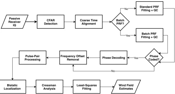
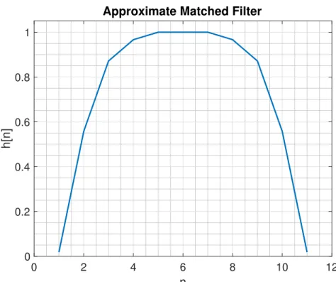
3.2 Flowchart depicting an overview of the signal processing scheme used to translate the passive radar time-series into wind field es-timates. CFAR detection is followed by a quality control process based on PRF-fitting. The frequency offset between transmitter and receiver is removed, and then estimates of power and velocity are calculated and localized to Cartesian coordinates. Finally the esti-mates are interpolated to a common grid and wind-field estimation is performed. Special WSR-88D transmit modes (batch PRF and SZ-2 coding) are detected and handled appropriately. . . 41 3.3 The approximate matched filter used to process the received time

series data. It was derived from experimental measurements of WSR-88D pulses. The half-power width of the approximate fil-ter is consistent with the 1.57µs nominal pulse length. The indexn

assumes a sampling rate of 5 MSPS. . . 42 3.4 In this segment of data collected from a transmitted WSR-88D

sig-nal, the rising edge of a direct-path pulse is located near sample 400. Note the drastically higher power levels due to ground clut-ter and weather afclut-ter the pulse in contrast to the samples collected prior. This severity of the issue is more striking given the context that the pulse itself is only about 8 samples long (1.57 µs at a 5 MSPS). . . 43 3.5 Measurements of direct-path pulse power over time. These pulses

form a repeating measurement of the WSR-88D beam pattern at changing elevation cuts based on the mechanical tilt of the transmitter. 45

(14)

3.6 This 0.44◦ elevation beampattern cut is taken from the same dataset used to produce Figure 3.5. Note the saturation of the main beam as well as the apparent irregularities in the sidelobe topography caused by strong ground clutter. . . 45 3.7 High-level outline of the PRF fitting process used to quality control

the pulse locations estimated by the CFAR detector. . . 46 3.8 Example of the “noisy sawtooth” form exhibited by the error

func-tionδ[n], as calculated from actual recorded data. Also shown is the error function recalculated after systematic error in samples-per-PRT has been corrected using the algorithm described in Section 3.1. 48 3.9 Rxample of measured pulse-to-pulse phase rotation distributions

af-ter decoding using each of the 8 possible delays. A delay of 2 sam-ples is clearly the correct option, as shown by the low variance of the resulting phases. . . 53 3.10 Example of a simulated pulse train spectrum, both with and without

a strong multipath interferer. Note that the peak of the macroscopic spectrum shown in the top plot shifts significantly due to the change in mainlobe shape induced by the multipath signal, but the locations of the individual “samples” visible at the finer scales shown in the lower two plots are virtually unaffected. This compares favorably with the measured data in Figure 3.11. . . 58

(15)

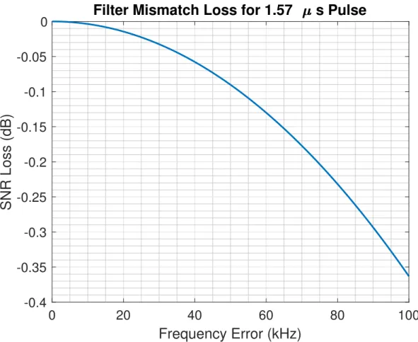
3.11 Example of two consecutive measured pulse train spectra with vary-ing multipath. It shows the same effect as in the simulations of Figure 3.10: significant peak movement at a macroscopic scale but extreme consistency at finer scales. Note that the smoothing and rapid rolloff of the expected sidelobes in the spectrum are due to low-pass filtering within the transceiver. . . 59 3.12 Loss in matched filter sensitivity due to errors in frequency estimation. 61 3.13 Example azimuthal pattern of the X-band proxy antenna used to

study the effects of pattern phase on velocity estimation biases. . . . 63 3.14 Results of the pattern phase error analysis across a range of rotation

rates and transmit antenna mechanical elevations. These results re-flect a 0.5 s data collection interval, and each plotted point corre-sponds to the worst possible result across the measureed antenna pattern range. . . 65 3.15 Block diagram of the passive radar hardware. . . 67 3.16 Normalized radiation patterns of the receiver antenna measured in

the ARRC far-field chamber. As the antenna is V-polarized, the E-plane corresponds to elevation, and the H-plane corresponds to azimuth. . . 68 3.17 An installed system on the roof of the Radar Innovations Lab at the

(16)

4.1 Raw estimates of range-corrected power (not reflectivity) and bistatic Doppler velocity obtained by the passive receivers, along with re-flectivity and radial velocity estimates from KTLX for comparison. The black contour illustrates the region selected for analysis based on the censoring criteria described in Section 4.1. The data shown were collected using a 4◦ elevation KTLX scan on April 6, 2019 at 16:11 UTC. Note that a ground clutter filter has not yet been ap-plied to these data, in order to more clearly show the logic behind the censoring boundaries. . . 72 4.2 Retrieved horizontal wind vectors over the analysis region. . . 73 4.3 Actual KTLX radial velocity field and the estimate of the KTLX

radial velocity obtained by projecting the retrieved horizontal wind field onto the vectors representing the pointing direction of KTLX at each point. . . 74 4.4 Results of the KTLX radial velocity retrieval are depicted here as

(a) spatial map of the root squared error in the retrieved estimate and (b) scatterplot of the relationship between the measured and retrieved values. The blue line in (b) represents a theoretical exact match between retrieved and measured values. . . 77

(17)

4.5 Raw estimates of range-corrected power (not reflectivity) and bistatic Doppler velocity obtained by the passive receivers, along with re-flectivity and radial velocity estimates from KTLX for comparison. The black contour illustrates the region selected for analysis based on the censoring criteria described in Section 4.1. The data shown were collected using a 4◦elevation KTLX scan on May 25, 2019 at 2:58 UTC. Note that a ground clutter filter has not yet been applied to these data, in order to more clearly show the logic behind the censoring boundaries. . . 79 4.6 Retrieved horizontal wind vectors over the analysis region. . . 80 4.7 These plots show the actual KTLX radial velocity field as well as

the estimate of the KTLX radial velocity obtained by projecting the retrieved horizontal wind field onto the vectors representing the pointing direction of KTLX at each point. . . 82 4.8 Results of the KTLX radial velocity retrieval are depicted here as

(a) spatial map of the root squared error in the retrieved estimate and (b) scatterplot of the relationship between the measured and retrieved values. The blue line in (b) represents a theoretical exact match between retrieved and measured values. . . 83

(18)

4.9 a) KTLX H-polarized reflectivity with analysis region outline and bistatic range contours corresponding to the RIL receiver b) KTLX H-polarized reflectivity with analysis region outline and bistatic range contours corresponding to the OUHSC receiver c) RIL re-ceiver range-corrected power with corresponding bistatic range con-tours and analysis region outline d) OUHSC receiver range-corrected power with corresponding bistatic range contours and analysis re-gion outline. See Figure 4.1 for a wider view of the same observa-tion set. . . 88 4.10 a) KTLX H-polarized reflectivity with analysis region outline and

bistatic range contours corresponding to the RIL receiver b) KTLX H-polarized reflectivity with analysis region outline and bistatic range contours corresponding to the OUHSC receiver c) RIL re-ceiver range-corrected power with corresponding bistatic range con-tours and analysis region outline d) OUHSC receiver range-corrected power with corresponding bistatic range contours and analysis re-gion outline. See Figure 4.5 for a wider view of the same observa-tion set. . . 90 5.1 High-level summary of the proposed pattern synthesis technique. . . 93 5.2 Example whitening pattern synthesis results for a 152 elementλ

/2-spaced ULA. The mask used is an approximation of the WSR-88D azimuth pattern at 0◦ elevation. Coding phase is the phase differ-ence between the two synthesized patterns to be used in the binary whitening scheme. Note that there is some deviation from ideal re-sults (0 in the mainlobe and π elsewhere), particularly within the first sidelobe and in the pattern nulls. . . 96

(19)

5.3 Evolution of the convergence criterionduring the synthesis of the pattern shown in Figure 5.2. It crosses the threshold value of 1×

10−12after 80 iterations. . . 101 5.4 Map showing which of the three possible whitening codes is applied

to each sidelobe region of a sample two-dimensional array pattern. . 102 5.5 Results of a 64 point whitening code used in conjunction with the

synthesized pattern. Doppler spectrum peak attenuation is the re-duction in the maximum Doppler spectrum value for an impingent clutter signal at each angle. As expected, near zero attenuation oc-curs in the mainlobe. . . 103 5.6 Several examples of the clutter signal Doppler spectra produced

us-ing the 64 point code (calculated with a Hammus-ing window). As anticipated based on the peak attenuations in Figure 5.5, the main-lobe spectrum receives virtually no spectral spreading, although the sidelobes are slightly perturbed relative to an ordinary Hamming window spectrum. The far sidelobe is extremely well whitened, with DC no longer having a dominant peak, and the first sidelobe spectrum lies between these extremes. . . 105 5.7 High-level view of the simulation process. The receiver-related

por-tion of the radar range equapor-tion calculapor-tion, as well as the sorting of scattering centers into range bins, are done prior to calculation of the transmitter-related weighting contributions. This structure maximizes the efficiency of the simulation process. . . 107

(20)

5.8 Gain patterns for each simulated transmitter scenario. Since the one-dimensional array factors of the two binary whitening patterns are identical, this means that the two-dimensional power pattern will remain constant during the whitening process and is also iden-tical to that of the unwhitened array pattern. . . 108 5.9 Constant-altitude slice of the NWP data grid used to produce the

simulation results. Reflectivity is shown in (a) while (b) and (c) show the zonal and meridional wind field components, respectively. The receiver and transmitter locations are also indicated, as well as a dashed line indicating the boundary of the observation region shown in Figures 5.10-5.11. . . 114 5.10 Doppler velocity fields measured by each reciever for each

simu-lated transmitter. There are significant errors due to sidelobe con-tamination in each image, primarily along areas of sharp reflectivity and velocity gradients. Note also regions of degraded spatial reso-lution along the transmitter/receiver baselines. . . 115 5.11 Differences between the dish, unwhitened array, and whitened

ar-ray simulations and the sidelobe-free ideal simulation. There are significant reductions in bias prevalence and magnitude between the dish and either of the arrays. Whitening provides a noticeable improvement compared to the unwhitened array. . . 116 5.12 Examples of the unwhitened, whitened, and ideal spectra from the

simulation results shown in Figure 5.10. The sidelobe leakage vis-ible in the unwhitened results is spread throughout the whitened spectrum, resulting in a closer match to the ideal results. . . 121

(21)

Abstract

Practical and accurate estimation of three-dimensional wind fields is an ongoing challenge in radar meteorology. Multistatic (single transmitter / multiple receivers) radar architectures offer a cost effective solution for obtaining the multiple Doppler measurements necessary to achieve such estimates. In this work, the history and fundamental concepts of multistatic weather radar are reviewed. Several develop-ments in multistatic weather radar enabled by recent technological progress, such as the widespread availability of high performance single-chip RF transceivers and the proliferation of phased array weather radars, are then presented. First, a net-work of compact, low-cost passive receiver prototypes is used to demonstrate a set of signal processing techniques that have been developed to enable transmit-ter / receiver synchronization through sidelobe radiation. Next, a pattransmit-tern synthesis technique is developed which allows for the use of sidelobe whitening to mitigate velocity biases in multistatic radar systems. The efficacy of this technique is then demonstrated using a multistatic weather radar system simulator.

(22)

Chapter 1 Introduction

Radar is among the most powerful and widely utilized technologies for remote ob-servation of the atmosphere. However, it is not without limitations. Prominent among these is the fact a single radar receiver is only capable of measuring the component of scatterer motion projected onto a single vector in three-dimensional space. For the most common case of a monostatic radar (a system in which the transmitter and receiver are colocated), this single vector extends radially along the pointing direction of the transmitter, giving rise to the familiar “radial velocity” product. Atmospheric motion, however, occurs in three dimensions, all of which are critical for understanding and predicting the weather. In order to completely reconstruct the motion of a given scatterer, it is necessary to measure its velocity along a minimum of three linearly independent vectors or to impose some additional constraints on scatterer motion using fluid dynamics. The desire for complete three-dimensional wind field reconstruction has, for this reason, given rise to the concept of multiple Doppler observations, in which two or more radar systems observe a

(23)

more directly and reduce dependence on theoretical constraints. One method of ob-taining multiple Doppler observations is the use of a multistatic (single transmitter / multiple receiver) radar network. The ultimate goal of the work presented here is to significantly decrease the expense and improve the practicality of these multi-static networks through the development of new signal processing techniques. This introduction seeks to contextualize that effort within the existing body of work on multiple Doppler data and methods, and on the radar systems used to obtain these types of measurements.

1.1 Multiple Doppler Observations With Monostatic

Radar

The concept of using a pulsed-Doppler radar for the purpose of measuring wind speed was first documented in a brief 1960Naturearticle by J.R. Probert-Jones [3]. This work merely notes the possibility that the radial component of wind velocity can be measured. Work over the subsequent decade gradually generalized single-radar wind field estimation using the concepts of Velocity-Azimuth Display (VAD) [4] and Volume Velocity Processing (VVP) [5], which can be useful for determin-ing the wind fields in the immediate surrounddetermin-ings of a sdetermin-ingle radar given certain assumptions on the homogeneity of both the wind field and hydrometeor size / fall speed in that area [6]. However, the problem of estimating the wind field in a region remote to a radar system inevitably required the coordination of two or more sys-tems. The first attempt at this problem was made by Lhermitte [7] for the simplified case limited to two radars and an assumed negligible contribution of hydrometeor fall speed to observed radial velocities. Armijo [8] expanded on this work by incor-porating the continuity equation into a multiple Doppler analysis. This allowed for

(24)

the assumption of known, rather than negligible, hydrometeor terminal velocities in the two radar case, and imposed no such assumptions for the three radar case, for which he also outlined an analysis procedure. Multiple Doppler wind field estima-tion has continued to evolve in the years since the Armijo paper, however the basic process remains recognizable. The radial velocities observed by a set of radars are combined with information about hydrometeor terminal velocity (typically derived from reflectivity) and/or the continuity equation. Innovation has come primarily in the form of improvements in how the resulting systems of equations are solved and in additional assumptions and constraints that can be added in order to reduce error. The analytic solution developed by Armijo requires an integration of the con-tinuity equation that is susceptible to undesirable levels of error accumulation [9]. In order to combat this effect, variational (least squares) methods have been em-ployed. These allow for the solution of an overdetermined problem, meaning that additional criteria such as smoothing constraints and multiple boundary conditions can be used to fit an optimal wind field estimate [10]–[12]. Iterative techniques have also been developed for the purpose of deriving solutions to these fitting prob-lems that will satisfy the continuity equation in a Cartesian coordinate system [9]. While these methods have been useful in improving the accuracy of radar-based wind field estimation, they do not address the fundamental challenges of temporal variation and coordination between radars - both critical in the collection of useful multiple Doppler observations.

Temporal variation in observed wind fields is problematic for multiple Doppler analysis due to the fact that (typically) radial velocity measurements throughout the analysis domain cannot be collected simultaneously. The wind field is evolv-ing while the measurements are beevolv-ing collected, which poses particular problems when attempting to apply the continuity equation or perform spatial interpolation

(25)

of sampled points onto a Cartesian grid. This effect is most dramatic between res-olution volumes that are adjacent in elevation, due to the azimuth-first scanning strategies of typical weather radars. This is a challenge even for the single-radar variety of wind field estimation, but it is exacerbated in the case of multiple radars. Not only should the data collected by each radar be contemporaneous with each other, but simultaneity is also desired between the samples collected by each of the different systems. While it is possible (although not necessarily simple) to coor-dinate radar operation in such a way that differences in temporal synchronization are minimized, exact agreement is quite impossible. Conical scans by two spatially separated radars can only overlap to a limited extent, and the problem is only ex-acerbated for larger networks. For this reason, advection correction techniques are used to rectify mismatches in temporal sampling, both within and between radar systems.

Chong et al. [13] suggest that temporal wind field variation associated with a storm be thought of as having two components: intrinsic variation consisting of evolution in the internal structure of the storm’s wind field, and advection con-sisting of the storm’s translational motion due to some uniform background wind field. Correction of the advection component is the most common and most readily achievable way to reduce errors due to temporal variation in the wind field. How-ever, sophisticated non-uniform advection correction methods have been developed in recent years [14], [15] that seek to address the intrinsic variation of the wind field. These techniques have been shown to improve advection correction perfor-mance compared to simple correction of uniform translational motion. However, they still suffer from limitations including sensitivity to the initial guess used to ini-tialize the process of correction optimization, as well as the possibility of temporal aliasing/non-uniqueness. In light of these limitations it is natural that engineering

(26)

solutions to the temporal variation problem have been sought. The use of a single-transmitter / multiple receiver radar network is one potential way to mitigate the problem of inter-radar scan synchronization.

1.2 Multistatic Weather Radar

Bistatic radar systems, in which the distance between the transmitter and receiver have a separation on the order of the target distance, have a long history in de-fense applications [16]. Initially, a bistatic radar presented a less radical change in architecture from a monostatic system as it does today, since the duplexer was not invented until 1936 [16]. Transmitters and receivers were separate by neces-sity until that point, even when colocated. Bistatic systems saw renewed interest in the modern era due in no small part to the advantages they offer in the context of electronic warfare. Most obviously, a transmitter inherently reveals its location, making a colocated receiver vulnerable to directive jamming or physical attack. By contrast, a bistatic receiver would remain hidden. Passive radar takes this concept a step further. These systems consist solely of a receiver that observes targets using signals transmitted by other radars or communications devices outside of its control. Interestingly, these concepts were key to some of the earliest radar experiments, which also had close ties to atmospheric science. The earliest experiments in radio direction-finding conducted by Robert Watson-Watt utilized passive receivers to lo-calize lightning strikes based on their associated microwave radiation [17]. When the British government requested a proof of concept demonstration before autho-rizing funding for the development of the first aircraft detection radar, Watson-Watt showed that the idea was feasible through passive radar observations using radio broadcast signals as an illumination source [18].

(27)

gan in earnest in the late 60s. The original focus of research in this area was on clear-air observations [19]. This is due to the fact that the reflectivity of a tur-bulent medium has a strong positive dependence on forward scatter angle. This allows clear-air observations using bistatic configurations at a much shorter wave-length than what would be realizable using a monostatic system. Subsequent ex-periments over the next few years produced bistatic measurements of scattering intensity from the melting layer [20], as well as successful bistatic Doppler mea-surements of precipitation [21]. The concept of using a single-transmitter / multiple receiver network for the collection of multiple Doppler weather observations was put forward in a 1993 paper by Wurman et al. [22]. The primary scientific advan-tage of this methodology is that it solves the inter-radar scan simultaneity problem, as the echoes from a given volume measured by each of the passive receivers orig-inate from the illumination of that volume by the transmitter at a common instant. This significantly reduces the complexity and potential for error introduced by the advection correction schemes needed to perform wind field estimation. The second major advantage of this architecture is economic; the cost of a multistatic network is miniscule compared to that of a monostatic radar network with the same number of sites. This is attributable to both the fact that the receivers do not need the elec-tronics necessary to produce a powerful transmit signal, and that they do not need the large antenna aperture necessary to form a highly directive beam.

The central problem of bistatic / multistatic radar design is how to achieve syn-chronization and coherence between the transmitting and receiving systems. This encompasses both carrier frequency synchronization, which must be extremely pre-cise in order to obtain accurate Doppler information, as well as pulse timing syn-chronization, which is necessary in order to accurately determine scatterer loca-tions. There is a spectrum of approaches available for achieving this kind of

(28)

syn-chronization. On one end of this spectrum is a set of cost and infrastructure inten-sive hardware-based solutions. Due to the fact that two free-running local oscilla-tors (LOs), which govern the carrier frequency at the transmitter and receiver, will drift relative to each other at levels that can cause significant errors in Doppler ve-locity estimation, some technique must be used to lock the LOs at the hardware level or correct for this drift in post-processing. The more expensive hardware-based syn-chronization solutions typically use GPS-disciplined oscillators in order to maintain carrier frequency synchronization. This is often complemented by communication of pulse-timing information over a dedicated communications channel between the transmitter and receiver [22]. This type of approach has the advantage of simplicity, precision, and low signal processing overhead. However, it has the disadvantages of more expensive hardware, strict specifications on the transmitter and receiver hardware, and potentially the need to tie receivers to a specific transmitter due to the communications infrastructure. A less hardware intensive approach [23] may involve using inexpensive hardware, for instance a free-running but high-quality ovenized oscillator, that is capable of maintaining acceptable stability over some temporary interval. The example in Wurman also eschews the use of a dedicated communications channel and achieves pulse timing synchronization through a man-ual tuning process in which the transmitting radar is pointed directly at the receiver and a human operator adjusts both the pulse timing and frequency parameters. Used in combination with a static pulse repetition time (PRT) at the transmitter, such a system could have both the frequency and pulse timing synchronization manually retuned at periodic intervals in order to ensure continued synchronization. This sys-tem, while less restrictive than the first, still poses some non-trivial requirements on hardware design and also requires significant human intervention, as well as con-trol over the transmitter for the purposes of conducting this manual tuning process.

(29)

Existing multistatic radars [22], [24]–[27] typically utilize the first technique which relies on GPS disciplined oscillators.

While the advantages offered by multistatic weather radar in terms of scan si-multaneity and system cost are undeniable, the architecture also presents some sig-nificant challenges for the collection of scientifically useful data [22]. One of these challenges is low sensitivity compared to monostatic radar. This problem arises from the fact that multistatic weather radar receivers typically utilize low-directivity antennas in order to allow for signal reception over a wide area without the need for beam steering. In contrast, a monostatic weather radar will have the advantage of a highly directive beam on both transmit and receive. The consequence of this is that the area over which a multistatic receiver has adequate sensitivity for data collection is relatively small. Another problem of multistatic networks is spatial variability in both spatial resolution and Doppler resolution. For reasons that will be explained in detail in Chapter 2, resolution in both space and Doppler frequency is significantly degraded for each receiver near the baseline between itself and the transmitter. This places a further limitation on the area over which a given receiver can collect use-ful observations. These limitations are, however, not of particularly grave concern. They are offset significantly by the extreme cost advantages offered by a multistatic architecture. Receive modules are sufficiently inexpensive that both the sensitivity and resolution concerns can be significantly mitigated merely through the instal-lation of additional receivers. Sensitivity concerns can be mitigated through the addition of receive modules at longer ranges from the transmitter, while resolu-tion concerns can be mitigated by the strategic addiresolu-tion of receive modules within the coverage area so as to achieve redundant coverage with non-overlapping trans-mit/receive baselines.

(30)

of sidelobe contamination. An additional effect of low-directivity receiver antennas is that the sidelobe levels will essentially be dictated by the one-way beam pattern of the transmitter. This can lead to extreme sidelobe contamination (particularly in areas of sharp reflectivity gradients) that can cause significant biases in velocity measurements. The complex geometries involved in this problem make compensa-tion through an increased number of receivers impractical. Some research on this topic has focused on studying and quantifying the severity of the problem [28] in order to allow for censoring based on contamination levels. Alternatively, Chong et al. [29] has proposed a technique for variational correction of the measured ve-locities based on precise knowledge of the antenna patterns. While this technique appears to be reasonably effective, it would be preferable to remove the bias at its source rather than through an approximate correction (much like correcting for tem-poral variation in multiple Doppler observations). Kawamura et al. [30] suggest a method to mitigate this effect with a receive antenna that has closely spaced narrow grating lobes. This does reduce sidelobe effects, but greatly reduces the observable area of the receiver to discrete non-contiguous angles. A more promising avenue for mitigation of this issue is sidelobe whitening [28], [31] (which will be discussed later), but this technique has been little studied up to this point.

1.3 Motivation

The objective of this work is to advance the state of the art in multistatic weather radar through the development of signal processing techniques that allow receive modules to automatically synchronize with any in-band coherent transmitter using only the direct-path radiation and time-stamped pointing angles. This synchroniza-tion method has a number of advantages over existing techniques that have relied on

(31)

and/or communicate information about precise pulse timings and transmit phases. By removing restrictions on oscillator quality, it further reduces the cost associated with receiver modules. More importantly, it removes many prohibitive restrictions on what transmitter may be used. Most existing weather radar systems can serve as viable candidate transmitters without any modification. This allows both further cost savings, and the ability to utilize the receivers in conjunction with systems over which one has limited or no access. To demonstrate this capability, the prototype receivers developed over the course of the work detailed here utilize the WSR-88D as the transmitter of opportunity. This capability has a number of implications. It certainly offers an appealing avenue for multiple Doppler field research for in-stitutions that may not have the considerable funding necessary to field multiple monostatic radars of their own. The interchangeability offered by the relaxation of requirements on transmitter hardware also makes this kind of system an intriguing choice for use in large field campaigns involving many monostatic systems. Receive units could theoretically switch seamlessly between transmitters involved in a given campaign based on need. The freedom from bulky oscillators and communications infrastructure also makes this type of receiver a good candidate for mounting on drones or for permanent/semi-permanent installation in elevated positions. Both of these strategies could be extremely useful for the collection of multiple Doppler data in rough or cluttered terrain (such as the southeastern United States). The prac-tical realities of beam blockage and locating feasible deployment locations in this type of environment have historically made the collection of multiple Doppler data in these areas extremely challenging.

One exciting possible application for this type of flexible synchronization tech-nique is to enable studies of the sidelobe whitening method for the mitigation of sidelobe contamination problem that has historically bedeviled multistatic weather

(32)

radar. This technique was first proposed by Sachidinanda and Zrni´c [31] for use in monostatic systems and was subsequently identified as a promising avenue for mit-igating the multistatic sidelobe problem by De Elia and Zawadski [28]. It involves perturbing the sidelobes of the transmitting antenna beam pattern on each pulse in order to decorrelate (and thereby mitigate) their contribution to Doppler velocity es-timates. The challenge is, of course, that this kind of sidelobe perturbation is really only practical for a phased array weather radar. Suitable prototype systems for im-plementation of this type of technique are only now becoming available. Prominent examples of suitable phased array radars include the Advanced Technology Demon-strator (ATD) [32], Polarimetric Atmospheric Imaging Radar [33] (PAIR), and Ho-rus [34]. If bistatic experiments demonstrating the efficacy of sidelobe whitening could be carried out using one or more of these systems, it would mark a potentially important development for multistatic weather radar. However, modification of the transmit electronics of these complex systems in order to make them suitable for use with more traditional multistatic weather radar hardware would be difficult or impossible. This makes the technology described in this dissertation an ideal tool for carrying out investigations into sidelobe whitening.

1.4 Outline

In Chapter 2, the fundamental theory of multistatic radars is outlined generally and then extended to the case of distributed scatterers in order to describe the oper-ation of multistatic weather radars. The signal processing scheme developed to allow automated transmitter/receiver synchronization through sidelobe radiation is described in Chapter 3. The hardware that comprises the prototype receiver mod-ules that have been constructed and deployed in the Oklahoma City, OK

(33)

metropoli-and discussion of weather observations using this prototype system. First, a set of velocities measured by the prototype systems is checked for consistency agains the radial velocities measured by KTLX, the nearest WSR-88D. Once this validation is presented, several additional cases of more significant meteorological interest are discussed. In Chapter 5, a new algorithm is described which makes the side-lobe whitening principle applicable to multistatic applications. Then a multistatic weather radar simulation framework is discussed and used to perform the first sim-ulations of the possible benefits of sidelobe whitening for mitigation of sidelobe contamination in multistatic weather radar networks. Finally, in Chapter 6, the con-clusions of this work are summarized and a number of possible avenues for further research are presented.

(34)

Chapter 2 Multistatic Weather Radar

Fundamentals

A bistatic radar can be defined as a radar system in which the distance between the transmitter and the receiver is on a similar order to the distance from a typical scatterer to the receiver. A multistatic radar system is an extension of this concept in which a group of at least two receivers with overlapping observation areas are deployed in conjunction with a single transmitter. Alternatively, a multistatic sys-tem can be implemented with a single receiver and multiple transmitters, but this is not common for weather radar applications. Typically, data from a multistatic radar network is processed by processing data from each transmitter / receiver pair, and then using a synthesis process to extract additional information beyond what is ob-servable by a single bistatic radar (such as three-dimensional velocity) and/or to use the additional measurements to reduce error in estimates of scatterer properties. In this chapter, descriptions of the fundamental physical properties and mathematical

(35)

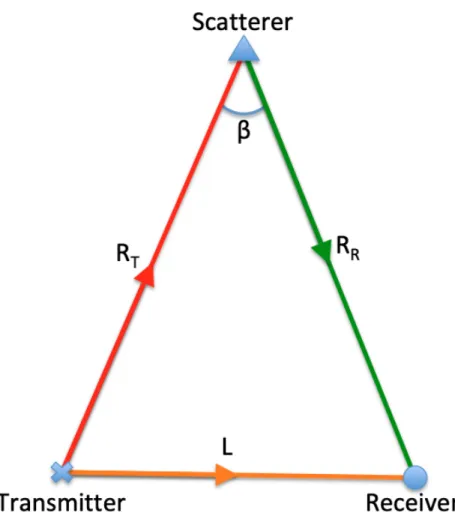
Figure 2.1: The fundamental geometry of a bistatic radar observation including the transmitter range RT, receiver range RR, baseline length L, and bistatic angle β.

The arrows indicate the direction of radiation propagation along each path. models of the multistatic radar observation process are provided.

2.1 Bistatic Radar Range Equation

In order to build an understanding of multistatic radar operation, it is useful to be-gin with a discussion of how an individual transmitter/receiver operates. Figure 2.1 shows a representation of bistatic radar geometry in the bistatic plane. It also intro-duces some key geometric variables that will be referenced frequently throughout this work. L is the baseline length, or the distance between the transmitter and

(36)

receiver. The transmitter rangeR_T is the distance between the transmitter and the scatterer under observation. Similarly, the receiver range RR is the distance

be-tween the receiver and the scatterer. Finally, the bistatic angleβ is defined as the angle between transmitter and receiver with a vertex located at the scatterer. The bistatic range, defined as RB = RT +RR, is another fundamental geometric

pa-rameter which appears frequently in mathematical models of bistatic systems and signals.

In a perfect analog to monostatic radar systems [35], a bistatic radar range equa-tion may be derived which relates the power emitted by the transceiver to that re-ceived by the receiver. The power density incident upon the scatterer is given by

Ss =

PTGTfT2(θTs, φsT)

4πR2

T

(W/m2), (2.1)

WherePT is the transmitted power,GT is the transmit antenna gain in the relative

direction of the scatterer, and f2

T(θTs, φsT) is the power pattern of the transmitter

antenna evaluated at the angular position (θs_T, φs_T) of the scatterer with respect to the transmitter . The radiated power is then reflected from the scatterer toward the receiver. The total scattered power in the direction of the receiver is

Ps=Ssσbi W, (2.2)

Whereσbiis the bistatic radar cross-section (RCS). This is a scatterer-specific

prop-erty determined by the composition and geometry of the scatterer. For a given scatterer, this value will vary dependent on the relative angular positions of the transmitter and receiver, as well as the polarization of the incident radiation. The

(37)

power density at the receiver will then be Sr = Ps 4πR2 R (W/m2). (2.3)

Given an effective antenna area Ae, the power measured by the receiver from a

scatterer located at its main beam peak is:

Pr=AeSr W. (2.4)

However, in the bistatic case, the relative position of the scatterer is unknown. This received power is therefore scaled byf2

R(θsR, φsR), the power pattern of the receiver

antenna evaluated at the angular position(θs

R, φsR)of the scatterer with respect to the

receiver, yielding: Pr =AeSrfR2(θ s R, φ s R) W. (2.5)

An antenna’s effective aperture can be related to its gain GR and operating

wave-lengthλbyAe =λ2GR/4π. Substituting that expression and equations (2.1)-(2.3)

into (2.5),Prcan be expressed as:

Pr = PTGTGRfT2(θsT, φTs)fR2(θsR, φsR)λ2σbi (4π)3_R2 TR 2 R W. (2.6)

2.2 Spatial Resolution

Because the focus of this work is on multistatic weather radar, it is desirable to generalize this radar range equation for point scatterers into a form appropriate for distributed scatterers, once again in a manner exactly analogous to the manner in which the same transformation is performed in the monostatic case. This is done by integrating the equation for point scatterers over some volume determined by

(38)

Figure 2.2: An example of the transmitter and receiver locations as the focii of an ellipse of constant range (shown in purple). This ellipse is a cross-section of the three-dimensional constant-range ellipsoid along the bistatic plane. For a scatterer located at any point on this ellipse, the bistatic rangeRB =RT+RRwill be constant.

the transmitter and receiver antenna patterns and the range resolution correspond-ing to the transmitted waveform bandwidth [36]. However, due to the additional geometric complexity of a bistatic system, the bistatic weather radar equation does not lend itself to a simple closed form expression (even with such simplifications as Gaussian beam patterns). In order to understand why this is so, it is necessary to discuss the characteristics of bistatic radar resolution volumes. The range quantity directly measured by a bistatic receiver isRB. This is obtained through the

relation-shipRB = c∆twhere ∆t is the time delay between the instant a pulse is emitted

by the transmitter and when the echo from the scatterer arrives at the receiver. The instant that the pulse is emitted is known through either dedicated communications infrastructure between the transmit and receive sites, or through monitoring of the direct path signal from from the transmitter. Using only the known value ofRB, it

(39)

Figure 2.3: The range and beamwidth boundaries that form a resolution volume in a typical bistatic weather radar. The concentric ellipses correspond to constant bistatic range ellipses. The translucent cones represent the main beam widths of the transmitter and receiver. The resolution volume formed by the intersection of the transmit beam with the ellipses is highlighted by a black dashed line.

a major axis ofRB. Figure 2.2 shows a cross-section of such an ellipsoid along the

bistatic plane (the plane passing through the scatterer, transmitter, and receiver lo-cations). The three-dimensional ellipsoid corresponds to a revolution of this ellipse about its major axis. Methods of determining the scatterer’s precise location on that ellipsoid will be discussed in Section 2.3. However, precisely as in the monostatic case, a given waveform only offers finite range resolution. Generally, this resolution is

(40)

∆r = c 2βw

m, (2.7)

whereβwis the bandwidth of the transmitted pulse. For a single-frequency,

unmod-ulated pulse, this resolution is

∆r= cτ

2 m, (2.8)

where τ is the temporal length of the pulse. This means that a resolution cell is bounded in range by two concentric ellipsoids representing two constant bistatic ranges with a difference of cτ /2. One notable feature is that the “thickness” of the shell formed by region between the constant range ellipsoids (measured along the direction of the bistatic bisector) is not constant, but rather depends on bistatic angle. There is not a convenient analytic expression for this variation although an exact but implicit solution exists. That solution is derived in [35] along with the following useful approximation:

∆R = ∆r

cos(β/2) m. (2.9)

This varying resolution cell thickness can be observed in the constant-range ellipses shown in Figure 2.3.

The cross-range boundaries of a resolution cell are defined by the antenna pat-terns of the transmitter and receiver. Because a typical multistatic weather radar architecture (including the one described in this work) uses a highly directive trans-mit antenna and a receive antenna with a broad non-directive beam, the simplifying assumption that the cross-range boundaries are defined exclusively by the transmit antenna pattern is reasonable. An illustration of the geometry of such a resolution volume is shown in Figure 2.3. It is important to note again that this representation

(41)

section of the conical transmit beam with the space between the two constant range ellipsoids determined by the range resolution associated with the transmitted wave-form. At this point, it may become evident where the difficulty lies in converting the bistatic radar equation to a distributed scattering form. In order to perform this con-version, the radar cross sectionσbi is replaced with an integral of reflectivityηover

the resolution volume weighted by the normalized transmit and receive antenna pat-ternsf_T2(θT, φT), fR2(θR, φR), as well as the range response|W(r)|2 associated with

the receiver transfer characteristic and transmitted waveform

σeff =

Z

V

f_T2(θT, φT)fR2(θR, φR)|W(r)|2ηdV m2, (2.10)

where θT, φT and θR, φR are the angles associated with spherical coordinate

sys-tems centered at the transmitter and receiver, respectively. For the monostatic case it is simple to make some reasonable approximations and arrive at a closed form expression for this quantity in terms ofη. This is because the resolution volume is simple to represent in terms of spherical coordinates with the origin located at the radar. Here, the antenna patterns are best represented by different spherical coor-dinate systems centered on the transmitter and receiver, while the range weighting function is best described by an elliptical coordinate system. The size and shape of the resolution volumes also changes dramatically depending on range and bistatic angle. This precludes the calculation of a convenient closed form solution for this integral in terms ofη, so this quantity will be represented asσeff(η, θT, φT, Rb). This

gives the bistatic weather radar equation the following form:

PR =

PTGTGRλ2σeff(η, θT, φT, Rb)

(4π)3_R2

TR2R

W. (2.11)

(42)

on range is effectively canceled by the corresponding increase in resolution volume size (while incident power density at the scatterers decreases asr2_{, the volume size}

increases asr2). The same general effect does, in fact, occur here; the solid angle of the isorange ellipsoidal shell intercepted by the transmitter beam is increasing with distance. However, the mathematical expression of this effect is not so clean as in the monostatic case. This is because the angle of incidence onto the shell is also dependent on bistatic range, which affects the size of the intercepted volume. However, the effect of this angular change approaches zero as the bistatic range goes to infinity. It is important to recognize that even though theRTvariable cannot

be precisely cancelled, bistatic weather radars are not somehow exempt from the general effects of increasing volume size on distributed scatter.

In order to extract calibrated values of η, the meteorological quantity of inter-est, from received power measurements using this range equation, the most viable avenue would be numerical computation due to the complex resolution volume geometries. However, the remainder of this work focuses almost exclusively on Doppler measurements, so this will not be discussed in detail. However, this dis-cussion of bistatic resolution volume variation and how it contributes to received power will be helpful in understanding some of the experimental measurements of received power shown in Chapters 3-4, as well as the simulation results in Chap-ter 5. A final aspect of this resolution volume variation that can be inferred from the discussion thus far, but deserves spatial mention, is the way that the resolution volume size degrades appreciably in regions near the baseline between the transmit-ter and receiver. This occurs due to loss of orthogonality between the beamwidth boundaries and the range boundaries. Along the baseline, this reaches its most ex-treme form. The entire baseline falls within a single resolution volume; this makes sense as there is no change in bistatic range regardless of where an object falls

(43)

Figure 2.4: Example of a degenerate resolution volume geometry in which the near bistatic range boundary is defined by the system baseline and the far bistatic range volume does not come into play, as the exterior volume edges are defined by the transmit and receive beampatterns.

along that line. An example of the kind of resulting degenerate geometry that can result from this effect is shown in Figure 2.4. In radar observations this will typi-cally manifest as a roughly elliptical distorted “blob” caused by the presence of any scatterers in the region subject to severe resolution volume degradation.

2.3 Echo localization

The simplest method by which to localize a received echo in a multistatic radar system is to employ a highly directive antenna at either the transmitter or receiver, and combine knowledge of the pointing angle of that antenna with the measured bistatic range. The point at which the directive antenna’s beam intersects the el-lipsoidal shell corresponding to the measured bistatic range is the target location. Assume a three-dimensional Cartesian coordinate system in which the scattering

(44)

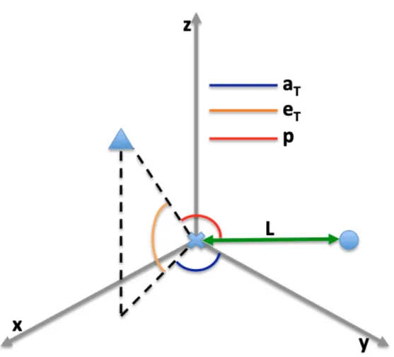
Figure 2.5: Diagram of the geometric quantities used to calculate Cartesian scatterer coordinates in (2.12)-(2.14).

(45)

particle is located at (x, y, z), a non-directive receiver is located at (L,0,0), and a highly directive transmitter is located at the origin. In this scenario, the particle location can be expressed as [22]:

x= R

2

B−L2

2[R_B−Lcos(p)]sin(aT) cos(eT), (2.12)

y= R 2 B−L2 2[RB−Lcos(p)] cos(aT) cos(eT), (2.13) z = R 2 B−L2 2[RB−Lcos(p)] sin(eT), (2.14)

whereaT andeT are the azimuth and elevation of the scatterer with respect to the

transmitter and p is the angle between the transmitter pointing direction and the baseline between the transmitter and receiver. These quantities are illustrated in Figure 2.5. The drawback of this technique is that processing cannot be performed without timestamped pointing angles from the transmitter. Using the WSR-88D as a transmitter of opportunity eliminates the possibility of real-time processing; it must wait until the WSR-88D data are publicly released. There does exist a tech-nique known as multilateration [35] which is used to localize scatterers observed by a multistatic network without any knowledge of the radiation pattern or point-ing angle of the transmitter. This technique, however, is not viable for use in the observation of distributed scatterers.

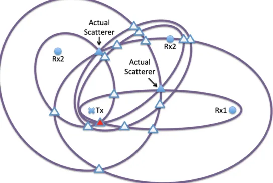
To demonstrate why, first consider Figure 2.6, which depicts the observation of a single scatterer by a multistatic network. Each receiver is capable of measuring a constant-range ellipse corresponding to the scatterer location. The places where these ellipses intersect represent candidate target locations. However, each pair of ellipses intersects twice. One of these locations corresponds to the actual scatterer, whereas the other is a spurious “ghost” target location. This ambiguity is resolved through the use of three simultaneous ellipses. The only location at which all three

(46)

Figure 2.6: Echo localization through multilateration in a network consisting of a single transmitter and three receivers. The purple ellipses represent isorange con-tours corresponding to detection of the actual scatterer by each receiver. If only two receivers are used, there will be two candidate detection locations where the isorange contours intersect: one at the location of the actual scatterer and a “ghost” represented by a white triangle. The third receiver is necessary for disambiguation.

(47)

Figure 2.7: Complications of multilateration when multiple targets are present. Ghost targets are represented by white triangles. The especially problematic ghost target at which three ellipses intersect is indicated in red.

ellipses intersect is the true scatterer location. An alternative technique to resolve these ambiguities is by checking for consistency in the Doppler information mea-sured by each transmitter / receiver pair. This type of technique can work well in the observation of a small number of discrete targets. However, there arises a problem of target association that renders this method increasingly impractical as the number of target-containing resolution volumes increases. A common weather scenario in which distributed scatterers filling an area of hundreds or thousands of contiguous resolution volumes represents an extreme case of this problem, which is why it is necessary to rely on information about transmitter pointing angle for the purposes of the system described in this work. Figure 2.7 depicts an illustration of this association problem in the simplest possible two-scatterer case.

(48)

con-tours corresponding to different scatterers. More problematically, it is even possible to have locations where three contours can intersect to create a ghost, making it sig-nificantly harder to distinguish from an actual scatterer. This issue is exacerbated by the fact that real systems have only finite range resolution, as discussed in Sec-tion 2.2, which means that the ellipses do not need to perfectly intersect to introduce ambiguity. The number of these ambiguities increases combinatorially with an in-crease in the number of scatterers present. Clearly, the presence of scatterers in tens of thousands of adjacent resolution volumes, as one might expect to see in weather radar applications, presents a completely intractable problem. Thus, we must rely on pointing angle knowledge for the localization of echoes from distributed scatter-ers.

2.4 Velocity Estimation

One feature that distinguishes bistatic from monostatic systems is the geometry involved with the measurement of Doppler velocities. It is well known that the Doppler velocity measured by monostatic systems is a radial velocity, or the pro-jection of the scatterer velocity vector onto the vector which represents the pointing angle of the radar system. Rather than measuring velocity along a radial corre-sponding to either the transmitter or receiver, bistatic systems measure velocity along the bistatic bisector. This is the vector bisecting the angle formed by the transmit and receive lines of sight to the scatterer. The Doppler frequency shift fd

measured by a bistatic system is, as in the monostatic case, the first time deriva-tive of the path length traveled by a pulse divided by its wavelength (assuming that acceleration over the observation interval is negligible). However, the separate transmit and receive paths must be accounted for in developing an expression for

(49)

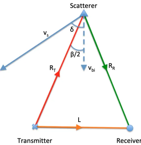
Figure 2.8: Relevant geometric quantities for modeling Doppler velocity measure-ments using a bistatic radar.

that quantity: fd = 1 λ d dt(RR+RT) Hz (2.15) = 1 λ dRR dt + dRT dt ) Hz, (2.16)

where λ is the operating wavelength of the transmitting radar. Consider then the geometry defined by Figure 2.8. Here,vs represents the total velocity of the

scat-terer, vbi is the projection of that velocity onto the bistatic bisector, and δ is the

angle between the scatterer’s direction of motion and the bistatic bisector. The time derivatives ofRRandRTcan be calculated by projectingvsonto the transmitter and

(50)

receiver lines of sight [35]: dRR dt =vscos δ+β 2 ms−1, (2.17) dRT dt =vscos δ−β 2 ms−1. (2.18)

Substituting these quantities into (2.16) yields

fd = vs λ " cos δ−β 2 + cos δ+β 2 # Hz, (2.19) = 2vs λ cos(δ) cos β 2 Hz. (2.20)

To describe what this equation represents conceptually, it is useful to consider it in three pieces. vscos(δ)is the projection of the scatterer velocity onto the bistatic

bisector. 2/λaccounts for the two-way path length change and converts the velocity in m/s to a frequency in rad/s through the division by λ. Finally, the cos(β/2)

is a scaling factor to account for spatial variation in the amount of path change produced by a given movement along the bistatic bisector. The necessity of this term is best illustrated through a consideration of the limiting cases. For a bistatic angle of0◦ in which the scatterer is colinear with the transmitter and receiver (but does not lie between them), an infinitesimal scatterer movement by a distancedr

along the bistatic bisector results in a path length change of2dr. However, given a bistatic angle of180◦ in which the scatterer lies on the baseline between transmitter and receiver, the bistatic bisector is orthogonal to the transmit and receive lines of sight. This means that a movement of dr along the bisector will produce no path length change whatsoever. This fact can be generally summarized by stating that the larger the bistatic angle becomes, the smaller the frequency shift induced

(51)

by a given v_bi. By extension, the larger the bistatic angle becomes, the larger the unambiguous Doppler velocity becomes, as the unambiguous Doppler frequency remains constant. However, because the frequency resolution of the receiver also stays constant, this means that the velocity resolution of the system degrades for large bistatic angles. This will occur in the region near the baseline, which is also the area subject to severe loss of spatial resolution due to loss of orthogonality between the isorange contours and transmitted beam.

2.5 Polarimetric Considerations

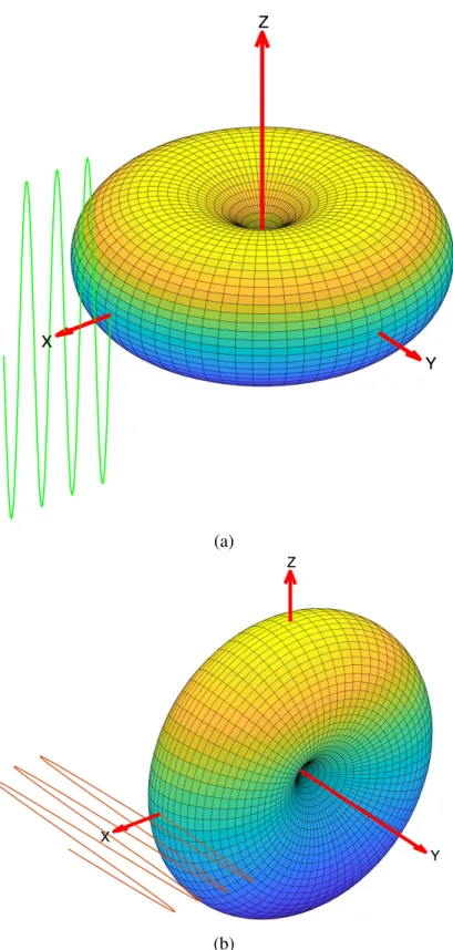
Another aspect of multistatic weather radar that must be considered is how polar-ization affects scattering behavior. While there has been some interest in bistatic weather radar polarimetry [37] for the purpose of discriminating and characterizing hail, the system described herein is single-polarization and designed specifically for wind field estimation. However, this aspect of bistatic weather radar is still impor-tant to the design of the system as it is desirable to design the polarization of the receive module antenna so as to optimize system performance. It has been shown [38] that the scattering behavior of liquid precipitation can be accurately modeled by assuming that each raindrop behaves as an electrically small dipole with a mo-ment vector oriented along the polarization direction of the impingent radiation. The consequences of this behavior are illustrated in Figure 2.9.

If the radiation is polarized along the z-axis, the RCS will be proportional to

sin2(θ) in a spherical coordinate system. In other words, the raindrop will have nulls in its bistatic RCS on the axis corresponding to the polarization of the im-pingent wave, and it will be omnidirectional about that axis. For the shallow ele-vation angles at which most weather obserele-vations are carried out, this means that H-polarized radiation will produce nulls in the scattered wavefront at90◦in azimuth

(52)

(a)

(b)

Figure 2.9: Three-dimensional bistatic RCS of raindrop with impingent radiation polarized along (a) the z-axis (V polarization) and (b) the y-axis (H polarization).

(53)

relative to the transmitter direction, as illustrated in Figure 2.9b. Any receivers lo-cated near those null angles will have degraded signal-to-noise ration (SNR) due to the weak scattering. This is undesirable, as such geometries produce excellent spa-tial and good Doppler resolutions, so it is not desirable to create blindness at those angles. By contrast, V-polarized radiation creates nulls directly above and below the raindrop. For most applications this is much more desirable, as scattering from the raindrop can be observed well by a receiver at any azimuthal position.

2.6 Wind Field Estimation

Once measurements ofvbihave been obtained, additional processing must be

per-formed to obtain an estimate of the observed wind fields in Cartesian coordinates. The basic process is to utilize some objective analysis method to interpolate the observations obtained by each radar system to a common grid and then to solve a system of equations to obtain each component of the wind vector at every point. While sophisticated techniques for wind field estimation such as those discussed in Chapter 1.1 can be applied to multistatic observations as readily as they may be applied to monostatic multiple Doppler data, such methods are beyond the scope of this work, which uses essentially the same simple techniques outlined in [22].

Objective analyses are used to take data obtained by multiple instruments on differing and irregularly spaced grids and estimate the state of those variables at common, regularly spaced points. This is a key stage in the pre-processing of data not only for wind field estimates such as those of interest here, but also for numeri-cal weather prediction and corresponding data assimilation processes. While mod-ern numerical weather prediction techniques typically use complex methods based in optimum control theory [39] to perform these estimates, several of the earliest and simplest interpolation-based techniques, such as the Barnes [40] and Cressman

(54)

-1 -0.8 -0.6 -0.4 -0.2 0 0.2 0.4 0.6 0.8 1 d 0 0.2 0.4 0.6 0.8 W(d) Cressman Weighting R_i=1

Figure 2.10: One-dimensional Cressman weighting function forRi = 1.

[41] techniques, are still widely used for multiple-Doppler analyses. The process-ing scheme used to obtain wind fields from multistatic observations collected for this work utilizes the Cressman technique. In this method, the value interpolated to each desired grid point is a weighted average of the available observations within some radius of influenceRi. The Cressman weighting function is

W(d) = R 2 i −d2 R2 i +d2 , (2.21)

where d is the distance between the desired grid point and the observation being weighted. The unit-radius Cressman weighting function in one dimension is shown in Figure 2.10.

Once the Cressman method or another objective analysis scheme has been used to interpolate the observations from each receiver to a common grid, the next step is to solve for the Cartesian velocity components at each point. For a monostatic radar system, the measured radial velocityvrcan be expressed in terms of the zonal

(55)

as follows [22]:

vr =usin(aT) cos(eT) +vcos(aT) cos(eT) +wpsin(eT) ms−1. (2.22)

A similar relationship exists for a bistatic velocity:

vbi =

sin(aR) cos(eR) + sin(aT) cos(eT)

2 cos(β/2) u+

cos(aR) cos(eR) + cos(aT) cos(eT)

2 cos(β/2) v +

sin(eR) + sin(eT)

2 cos(β/2) w ms

−1_.

(2.23)

It is clear that in either the monostatic or multistatic case (or a combination), at least three independent velocity measurements are necessary to solve for the three components of the wind field. For a multistatic network consisting of a single trans-mitter (with accompanying receiver allowing it to function as an independent mono-static radar) and multiple receivers, the corresponding system of equations can be represented in matrix format as:

           

sin(a1) cos(e1)+sin(aT) cos(eT)

2 cos(β1/2)

cos(a1) cos(e1)+cos(aT) cos(eT)

2 cos(β1/2)

sin(e1)+sin(et)

2 cos(β1/2)

sin(a2) cos(e2)+sin(aT) cos(eT)

2 cos(β2/2)

cos(a2) cos(e2)+cos(aT) cos(eT)

2 cos(β2/2)

sin(e2)+sin(eT)

2 cos(β2/2) ..

. ... ...

sin(aN) cos(eN)+sin(aT) cos(eT)

2 cos(βN/2)

cos(aN) cos(eN)+cos(aT) cos(eT)

2 cos(βN/2)

sin(eN)+sin(eT)

2 cos(βN/2)

sin(aT) cos(eT) cos(aT) cos(eT) wpsin(eT)

                 u v w      =             vbi1 vbi2 .. . vbiN vr             , (2.24)

Multistatic Passive Weather Radar

Acknowledgments

IEEE Copyright Notice

Table of Contents

List of Figures

Abstract

Chapter 1

Introduction

1.1

Multiple Doppler Observations With Monostatic

Radar

1.2

Multistatic Weather Radar

1.3

Motivation

1.4

Outline

Chapter 2

Multistatic Weather Radar

Fundamentals

2.1

Bistatic Radar Range Equation

2.2

Spatial Resolution

2.3

Echo localization

2.4

Velocity Estimation

2.5

Polarimetric Considerations

2.6

Wind Field Estimation