No. 426
August 2015 (Revised, October 2015)
www.carloalberto.org/research/working-papers
The increase of the gender wage gap in Italy
during the 2008-2012 economic crisis
∗
Daniela Piazzalunga
†1, 2, 3and Maria Laura Di Tommaso
‡1, 2, 41Department of Economics and Statistics ‘Cognetti de Martiis’, Universit`a di Torino, Lungo Dora Siena 100A, 10153 Torino, Italy
2CHILD Collegio Carlo Alberto, Italy 3LISER, Luxembourg
4Collegio Carlo Alberto, Italy
Abstract
The paper examines the gender wage gap in Italy during the 2008-2012 economic crisis, using cross-sectional EU-SILC data. The gender wage gap increased from 4% in 2008 to 8% in 2012, while for most European countries the gap decreased over the same period. After 2010 the growth of the Italian gender wage gap (and its unexplained component) was particularly high in the upper part of the wage distribution. In 2010-2011 a wage freeze in the public sector was introduced as an austerity measure, and the average public sector premium dropped from 15% to 11%. Using counterfactual analyses, we show that the wage freeze has been one of the major causes of the growth of the gender wage gap, disproportionately affecting women, who are more likely to be employed in the public sector. This ‘policy effect’ accounts for more than 100% of the increase between 2009 and 2011, while other changes, if anything, would have reduced the gender gap.
JEL:J31, J71, J16, J45
Keywords: Gender wage gap, Great recession, Public sector premium, Decompo-sition, Counterfactual analysis
∗We are grateful to Karina Doorley for very useful suggestions. We also want to thank Leif Andreassen, Alessio Fusco, Ronald Oaxaca, Raul Ramos, Mariacristina Rossi, Eva Sierminska, Steinar Strøm, Philippe Van Kerm for helpful discussions and comments, as well as the participants at the ‘Equal Pay: Fair Pay? A forty-year perspective’ symposium in Cambridge, 2014 EALE Conference in Ljubljana, and at the seminar at LISER in Luxembourg. We thank Collegio Carlo Alberto for financial and technical support. Part of this research was conducted while Daniela Piazzalunga was visiting LISER, and she would like to acknowledge their hospitality. A previous version of this paper was circulated under the title: ‘It is not a bed of roses: Gender and ethnic pay gaps in Italy’.
1
Introduction
The gender wage gap (GWG) in Italy is lower than in other European countries. The unadjusted gender wage gap was 7.3% in 2013, while the European average was 16.4% (Eurostat, 2015). Furthermore, some studies suggest that the impact of the current eco-nomic crisis has been less serious for women than for men. In the US, men experienced higher probabilities to lose their jobs and higher unemployment rates than women (Siermin-ska and Takhtamanova, 2011). In Europe, Bettio et al. (2013) show that men in countries with a high level of gender segregation had higher levels of employment losses than women. In addition, they find that the gender pay gap decreased for most European countries. In Italy, the unemployment rate is still higher for women (13.8% in 2014) than for men (11.9% in 2014), but the difference has decreased since 2008 (Istat, 2015). The gender pay gap increased during the economic crisis of 2008-2012.
Despite the increased monitoring of the gender wage gap by the European Union and by international organizations (e.g. Eurostat, 2015), economic research on the gender pay gap in Italy has been relatively scarce, although increasing in recent years. Some studies compare the Italian gender pay gap with other European countries (Olivetti and Petrongolo, 2008; Nicodemo, 2009; Christofides et al., 2013), others link the gender pay gap to educational attainment (Addabbo and Favaro, 2011; Mussida and Picchio, 2014a), showing that the gender wage gap is larger among people with low education, while Del Bono and Vuri (2011) analyse how gender differences in job mobility affect the gender wage gap. Mussida and Picchio (2014b) compare the gender wage gap in Italy in the mid-1990s and in the mid-2000s. They show that over time the gender gap is pretty stable, but the underlying components change: while women’s qualifications would have reduced the gap, the changes in returns increased it, in particular at the top part of the distribution. To the best of our knowledge, there are no studies about the GWG during the recession. However, the economic crisis could affect the GWG through changes in the labour market and austerity measures.
In this paper, we study the gender earnings gap in Italy and its change during the 2008-2012 economic crisis utilising the European Union Statistics on Income and Living Conditions (EU-SILC) from 2004 until 2012. Figure 1 shows that the unadjusted gender gap in hourly wages has been decreasing from 9% in 2004 to 4% in 2008. However, since 2008, the gender wage gap increased steadily, and in 2012 it was almost back at the level of 2004 (8.1%)1.
1Estimations of the GWG from EU-SILC data are not exactly comparable with those provided by
Figure 1: Gender wage gap in Italy, 2004-2012 0 2 4 6 8 10 12 Gap 2004 2005 2006 2007 2008 2009 2010 2011 2012 Unadjusted gender wage gap 95% confidence bands
Gross wages per hour in 2008 real price. Source: EU-SILC, own calculations.
In order to analyse the gender pay gap in more detail, we first apply the Oaxaca-Blinder methodology, which decomposes the gender pay gap into an explained component (due to gender differences in characteristics) and a residual unexplained component. We also take into account self-selection in participation. Then we apply a quantile decomposition to analyse the gap along the wage distribution. We show that the GWG is completely unexplained by observed characteristics and that, after 2010, the GWG is particularly high in the upper part of the wage distribution.
Next, we utilise counterfactual analyses to study the effect of the wage freeze in the public sector (a large employer of women). In Italy, public sector wages were frozen in 2010-2011, due to an austerity measure to reduce the public debt: consequently, the average public sector premium significantly dropped from 15% in 2010 to 11% in 2011, with an even more pronounced drop for women. The counterfactual analyses show the public sector wage freeze contributed to the increase in the gender wage gap. Finally, we analyse some of the changes within the public sector looking at the different effects of the austerity measures on different sub-sectors (education in particular).
The fact that in Italy the gender effects of austerity measures have been overlooked is consistent with the absence of gender mainstreaming in evaluating economic policies (Villa
and Smith, 2010). In addition, Italy has a long history of gender disadvantages. The female participation rate was only 54% in 2014, still very low with respect to other European coun-tries (Istat, 2015), and is one of the causes of the low gender pay gap, because of the positive self-selection of women into the labour force (Olivetti and Petrongolo, 2008). Among OECD countries, Italy has the highest gender gap in leisure time: Italian men enjoy 80 minutes more of leisure time per day than Italian women (OECD, 2009). In fact, Italian women perform 76.2% of domestic and care work (Istat, 2010)2.
The rest of the paper is organized as follows: section 2 discusses the details of the public sector wage freeze. Section 3 describes the dataset and provides some descriptive statistics. Section 4 illustrates the trend in the gender wage gap in Italy, using both the Oaxaca-Blinder and the quantile decompositions. Section 5 investigates the role of the wage freeze in the public sector on the gender wage gap, while section 6 analyses the changes within the public sector itself. Finally, section 7 concludes.
2
Austerity measures and the public sector wages
The economic crisis struck Italy at the end of 2008, and again in 2011 with the sovereign debt crisis. Italy adopted different austerity measures in successive waves, many of them devoted to reducing public spending, affecting the public sector employment levels and wages (Bordogna, 2013; Figari and Fiorio, 2015).
From 2010, three main types of provisions were enforced (Bordogna and Neri, 2012): cuts in the number of public employees through very tight replacement ratios; reform of the pension system (both for private and public employees); and measures to limit the wages of public employees. The latter consisted in a freeze of the 2010-2012 base wage bargain-ing round at national level. Collective negotiations at national level were abolished by the decree law n.78/2010 (law 122/2010, into force since January 2011). In addition, the above-mentioned law forbids individual wages to exceed the level of 2010, also preventing wages’ increases due to career promotions, with the partial exception of the component linked to merit or performance pay. Later these measures were extended until the end of 2014.
Financial constraints introduced by the national government meant also,de facto, a freeze in wages negotiations at the local level. Rules were also adopted preventing any salary increase due to seniority or career promotion for non-contractualized personnel (such as
2These facts also mirror the opinions of Italians with respect to gender-related topics (European
prefects, university professors, police and armed forces, judges).
Moreover, according to Bordogna and Neri (2012, p.15) ‘most of these measures have been unilaterally adopted by the government, without previous negotiations with trade unions and without searching union consent; in some cases, explicitly against trade union protests’.
These measures substantially froze public wages at the level of 2010, without the pos-sibility of recovering the losses at the end of the period, and also with effects on future pension payments. In addition there were wage cuts for higher level salaries, by 5% for those with a yearly gross wage between 90,000e and 150,000e, and by 10% for the part exceeding 150,000e (Bordogna and Neri, 2012; Tronti, 2011)3.
Among employees at public schools and universities, automatic seniority wage increases were cancelled (such increases were already abolished in the rest of the public sector at the end of the 90’s).
As a result of these measures, public sector real hourly wages decreased on average by 9.1% between 2010 and 20124. Women’s hourly wages decreased by 11.5% from 2010 to 2012, while they decreased by 6.2% for men (see Figure 2).
Figure 2: Hourly wages: public and private sector, by gender, 2004-2012
9 10 11 12 13 14 15
Hourly real wages
2004 2005 2006 2007 2008 2009 2010 2011 2012 Year
Men, Private sector Women, Private sector Men, Public sector Women, Public sector
Gross wages per hour in 2008 real price.
The dotted vertical lines refer to the beginning of the economic crisis (2008) and to the implementation of the wage freeze (2011).
Source: EU-SILC, own calculations.
3In our data, 99.5% of men earn less than 90,000eper year, and only the 0.03% earn more than 150,000e.
99.9% of women earn less than 90,000e and none earn more than 150,000e. Hence, only a very small percentage of people in our sample is concerned by those cuts. Still, if anything, they should have reduced the gender wage gap, since more men than women have top wages.
3
Data and descriptive statistics
The analysis is based on the Italian sample of EU-SILC (European Union Statistics on In-come and Living Conditions) for 2004-20125. In the full sample there are about 40,000-50,000 observations per year. We select 20-65 years old6 employees, with Italian citizenship7. We
exclude individuals who are inactive, unemployed, retired, self-employed, or family workers. We also lose about 300 observations per year because the wage is missing. The final number of observations ranges between 16,635 (2004) and 11,722 (2012). Table A.1 in the Appendix summarizes the selection procedure.
When we take into account self-selection in participation, using the Heckman procedure, the sample is larger, including 20-65 years old employed, unemployed and non-employed people. We still exclude self-employed and employed people but with no information about wages. The total number of observations ranges between 30,474 (2004) and 20,984 (2012).
The main dependent variable is the (log) hourly wage, which is the gross monthly wage divided by the number of hours usually worked per month - included usual overtime - and it refers to the year of the survey. All wages are expressed in 2008 real prices. Table A.2 in the Appendix provides the detailed definitions of all dependent and control variables.
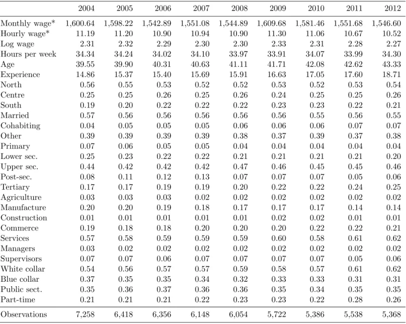
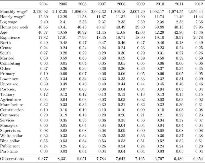
Tables 1 and 2 show descriptive statistics for women and men. Average real wages have constantly fallen since 2009, for both men and women. A larger share of women than men held a tertiary degree in 2004 (respectively 17% and 12%), and the gap in the education achievements widens even more over time: in 2012, 25% of employed women has a university degree, versus 15% of men.8
5One of the best dataset to conduct labour market analysis is the Italian Labour Force Survey (LFS),
but it does not provide good information to evaluate wages: wages in LFS are truncated from below at 250e and at 3,000e from above. To analyse the gender pay gap it is essential to have the whole distribution of wages and in particular the top ones.
Alternatively, Eurostat (2015) uses the Structure of earnings (SES) survey. However, SES data are available only for (1995), 2002, 2006, 2010, thus the last wave available is before the wage freeze. Moreover, with data available only every four years, it is difficult to identify the entire trend. Finally, before 2010, NACE sector O (Public administration and defence) was not included.
6Using different age groups (e.g. 25-55) yields to very similar results.
7The gender wage gap for foreign people can be different (see, for instance, Piazzalunga (2015) for an
analysis of the gender gap among immigrants in Italy). Moreover, non-Italian citizens cannot work in the public sector.
8The gap in education exists also in the full sample, including non-working people, as can be seen from
Table 1: Descriptive statistics - Employed Italian women (20-65 yo), 2004-2012
2004 2005 2006 2007 2008 2009 2010 2011 2012
Monthly wage* 1,600.64 1,598.22 1,542.89 1,551.08 1,544.89 1,609.68 1,581.46 1,551.68 1,546.60 Hourly wage* 11.19 11.20 10.90 10.94 10.90 11.30 11.06 10.67 10.52
Log wage 2.31 2.32 2.29 2.30 2.30 2.33 2.31 2.28 2.27
Hours per week 34.34 34.24 34.02 34.10 33.97 33.91 34.07 33.99 34.30
Age 39.55 39.90 40.31 40.63 41.11 41.71 42.08 42.62 43.33 Experience 14.86 15.37 15.40 15.69 15.91 16.63 17.05 17.60 18.71 North 0.56 0.55 0.53 0.52 0.52 0.53 0.52 0.53 0.54 Centre 0.25 0.25 0.26 0.25 0.26 0.24 0.25 0.25 0.26 South 0.19 0.20 0.22 0.22 0.22 0.23 0.23 0.22 0.21 Married 0.57 0.56 0.56 0.56 0.56 0.56 0.55 0.56 0.55 Cohabiting 0.04 0.05 0.05 0.05 0.06 0.06 0.06 0.07 0.07 Other 0.39 0.39 0.39 0.39 0.38 0.37 0.39 0.37 0.38 Primary 0.07 0.06 0.05 0.05 0.04 0.04 0.04 0.04 0.04 Lower sec. 0.25 0.23 0.22 0.22 0.21 0.21 0.21 0.21 0.20 Upper sec. 0.44 0.42 0.42 0.42 0.47 0.46 0.45 0.45 0.46 Post-sec. 0.08 0.11 0.12 0.13 0.07 0.07 0.07 0.05 0.06 Tertiary 0.17 0.17 0.19 0.19 0.20 0.22 0.22 0.24 0.25 Agriculture 0.03 0.03 0.03 0.02 0.02 0.02 0.02 0.02 0.02 Manufacture 0.20 0.20 0.19 0.18 0.17 0.17 0.17 0.14 0.14 Construction 0.01 0.01 0.01 0.01 0.01 0.02 0.02 0.01 0.01 Commerce 0.19 0.18 0.18 0.20 0.20 0.20 0.22 0.22 0.21 Services 0.57 0.58 0.59 0.59 0.59 0.60 0.58 0.61 0.62 Managers 0.03 0.02 0.02 0.02 0.02 0.02 0.02 0.02 0.02 Supervisors 0.07 0.07 0.06 0.07 0.07 0.07 0.07 0.05 0.06 White collar 0.54 0.56 0.57 0.57 0.59 0.58 0.57 0.61 0.62 Blue collar 0.37 0.35 0.35 0.34 0.32 0.33 0.33 0.31 0.31 Public sect. 0.35 0.36 0.37 0.36 0.36 0.35 0.34 0.35 0.35 Part-time 0.21 0.21 0.21 0.22 0.23 0.23 0.22 0.28 0.26 Observations 7,258 6,418 6,356 6,148 6,054 5,722 5,386 5,538 5,368 * Gross wages in 2008 real prices.
Table 2: Descriptive statistics - Employed Italian men (20-65 yo), 2004-2012
2004 2005 2006 2007 2008 2009 2010 2011 2012
Monthly wage* 2,120.92 2,107.25 1,986.63 2,002.32 1,948.18 2,007.29 1,992.17 1,974.55 1,959.44 Hourly wage* 12.30 12.29 11.58 11.67 11.32 11.90 11.74 11.49 11.44
Log wage 2.40 2.41 2.36 2.37 2.35 2.39 2.38 2.35 2.35
Hours per week 40.66 40.41 40.43 40.47 40.49 39.50 39.88 40.13 39.95
Age 40.37 40.58 40.92 41.45 41.68 42.03 42.29 42.80 43.36 Experience 17.82 17.81 17.99 18.45 18.71 18.90 19.10 19.97 20.78 North 0.49 0.48 0.47 0.47 0.46 0.47 0.46 0.48 0.49 Centre 0.24 0.24 0.24 0.24 0.24 0.23 0.23 0.24 0.25 South 0.27 0.28 0.29 0.29 0.30 0.29 0.31 0.27 0.26 Married 0.60 0.59 0.60 0.60 0.59 0.59 0.58 0.59 0.59 Cohabiting 0.03 0.05 0.04 0.05 0.05 0.05 0.06 0.06 0.06 Other 0.37 0.36 0.36 0.36 0.36 0.36 0.37 0.35 0.35 Primary 0.10 0.09 0.07 0.06 0.06 0.05 0.06 0.05 0.05 Lower sec. 0.35 0.34 0.34 0.33 0.33 0.33 0.32 0.31 0.29 Upper sec. 0.39 0.39 0.40 0.40 0.44 0.44 0.45 0.46 0.46 Post-sec. 0.05 0.07 0.08 0.08 0.04 0.04 0.04 0.03 0.04 Tertiary 0.12 0.12 0.12 0.13 0.13 0.13 0.13 0.15 0.15 Agriculture 0.04 0.04 0.03 0.03 0.03 0.02 0.03 0.03 0.02 Manufacture 0.32 0.33 0.32 0.32 0.31 0.32 0.32 0.30 0.31 Construction 0.10 0.10 0.10 0.10 0.10 0.09 0.10 0.08 0.08 Commerce 0.20 0.19 0.19 0.20 0.20 0.21 0.21 0.22 0.23 Services 0.33 0.35 0.36 0.36 0.35 0.36 0.34 0.37 0.37 Managers 0.06 0.05 0.04 0.04 0.04 0.04 0.04 0.04 0.04 Supervisors 0.08 0.08 0.08 0.08 0.09 0.09 0.08 0.08 0.08 White collar 0.32 0.33 0.34 0.35 0.35 0.36 0.36 0.37 0.38 Blue collar 0.55 0.53 0.54 0.53 0.53 0.51 0.52 0.52 0.51 Public sect 0.24 0.25 0.25 0.26 0.24 0.24 0.24 0.24 0.23 Part-time 0.03 0.03 0.04 0.04 0.04 0.04 0.03 0.05 0.04 Observations 9,377 8,331 8,051 7,784 7,642 7,165 6,767 6,489 6,354 * Gross wages in 2008 real prices.
The change in the composition of the labour force is one of the possible reasons sug-gested as a cause of the increase in the Italian gender gap (see, for instance, Bettio, 2013). This change could also lead to some concerns about our estimations. This could happen through the added worker effect or if mainly low-paid men have lost their job during the crisis. Considering the average characteristics of working people (Tables 1 and 2), the main differences are the increase in average age (and consequently in experience) and in the level of education. The same patterns are also evident in the total population aged 20-65 (Tables A.3 and A.4), which means that they mainly reflect the ageing of the population and its increasing education level. However, workers are ageing faster than the general population. In the total population, individuals in 2012 are on average 2 years older than in 2004, while among employed people they are about 3 years older. Nonetheless, both in the total popu-lation and among employed people the trend has not changed since 2004. Hence, it seems that older people - both men and women - have been slightly more likely to be employed than younger ones in the past decade, both before and during the economic crisis. Overall, this suggests that, even though a (small) added worker effect took place (Bredtmann et al., 2014; Ghignoni and Verashchagina, 2014), it has not affected the average characteristics of the stock of working women. Nevertheless, we also present results corrected for self-selection into the labour market.
Similarly, while it is true that at least in the first years of the crisis more men than women lost their jobs (Istat, 2015), there is no significant change in the composition of the stock of the labour force. Moreover, the distribution of wages for men did not change, as shown in Figure 3. If anything, the wage distribution changed for women. Between 2008 and 2012, the wages of women in the upper part of the distribution decreased.
Since the average wages were stable for both men and women working in the private sector (Figure 2), these women are probably those employed in the public sector, who were disproportionately affected by the wage freeze of 2011. Indeed, more women are employed in the public sector than men (respectively about 35% and 24%). These percentages have been stable over time, even after the wage freeze of 2011, or the aforementioned reduction in hiring (Tables 1 and 2).
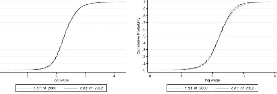
When we consider only people employed in the public sector, the cumulative distribution functions show that wages for high income individuals have been falling between 2008 and 2012 among both men and women (Figure 4), but the fall among women was larger.
Descriptive statistics for the public sector are shown in Tables A.5 and A.6. Both men and women are better educated than the total sample, and they are slightly older than average. In 2012, 40% of women had a university degree, against 30% of men. Women
Figure 3: CDF log wages, 2008-2012 0 .1 .2 .3 .4 .5 .6 .7 .8 .9 1 Cumulative Probability 0 1 2 3 4 log wage c.d.f. of 2008 c.d.f. of 2012 Men 0 .1 .2 .3 .4 .5 .6 .7 .8 .9 1 Cumulative Probability 0 1 2 3 4 log wage c.d.f. of 2008 c.d.f. of 2012 Women
Log in 2008 real price. Source: EU-SILC, own calculations.
Figure 4: CDF log wages, Public sector, 2008-2012
0 .1 .2 .3 .4 .5 .6 .7 .8 .9 1 Cumulative Probability 0 1 2 3 4 log wage c.d.f. of 2008 c.d.f. of 2012 Men 0 .1 .2 .3 .4 .5 .6 .7 .8 .9 1 Cumulative Probability 0 1 2 3 4 log wage c.d.f. of 2008 c.d.f. of 2012 Women
Log in 2008 real price. Source: EU-SILC, own calculations.
are mainly employed in the education sector (42% in 2012), while most men work in public administration and defence (48% in 2012).
4
Long-term changes in the gender wage gap
4.1
Oaxaca-Blinder decomposition
To analyse the evolution of the gender wage gap during the economic crisis, we start ap-plying the standard Oaxaca-Blinder decomposition (see Oaxaca, 1973; Blinder, 1973), which divides the wage gap into an explained component based on observed characteristics and an unexplained residual component.
We first estimate the following linear wage equation, separately for men (m) and women (f):
lnWgt =βgtXgt+vgt =δgtZgt+γgtP U BLICgt+etg (1) where t= 2004,2005, ...,2012 and g ={m, f}.
The dependent variable is the log hourly wage (Wgt), Xgt is the vector of observable characteristics (age, age squared, experience, experience squared, region of residence, marital status, level of education, sector of employment (Nace), position, public sector, part-time job9), βt
g are the coefficients to be estimated with OLS and vtg is a stochastic term. In the second part of eq. 1, we isolate the coefficient associated with working in the public sector γt
g (i.e. ‘public sector premium’), where P U BLIC is a dummy equal 1 if the person works in the public sector, and Zt
g are the remaining controls.
One issue that can arise is self-selection. Indeed, it is widely recognized that the gender wage gap in Italy is also affected by the low participation of women in the labour market (Olivetti and Petrongolo, 2008). Once that is taken into account, the gender wage gap is usually larger. Moreover, during the economic crisis the participation of women may change because of the added worker effect. Some women entered into the labour market to compensate for the job loss of their husbands (Bettio, 2013; Ghignoni and Verashchagina, 2014). We apply the Heckman-correction to account for self-selection into the labour market (Heckman, 1974), including the number of children in the selection equation as an exclusion restriction (also controlling for age, region of residence, marital status, and level of education).
9We also controlled for the type of contract (i.e. temporary contracts) in an alternative specification, and
A similar issue should be considered with respect to the public sector (e.g. Depalo et al., 2015). People may select themselves into the private or the public sector, depending on unobserved characteristics or preferences. However, for the purpose of our paper, we do not correct for self-selection into the two sectors. In our data there is no useful information which may predict such a choice, and which does not affect wages10. We rely on the assumption that self-selection in the public sector did not change over the 2008-2012 period, or, at least, that the public sector premium was not affected by individual choices (wages in the public sector are highly regulated).
Another issue - which may affect the gender wage gap - is that the characteristics of people losing their job (and in particular men) may not be random. We have shown in the descriptive statistics (section 3) that this last issue is not a problem.
The Oaxaca-Blinder is given by:
GW Gt = lnWtm−lnWtf = (Xtm−Xtf) ˆβt m+X t f( ˆβmt −βˆft) (2)
The first term refers to differences in characteristics (explained component), while the second term is the so-called unexplained component, due to differences in returns. We use the coefficients for males, ˆβt
m, as benchmarks, to have results comparable with the Heckman-corrected ones and with the quantile decomposition11.
When we apply the Heckman-correction, we decompose the observed gender wage gap into an explained, an unexplained, and a selection component, following Neuman and Oaxaca (2004).
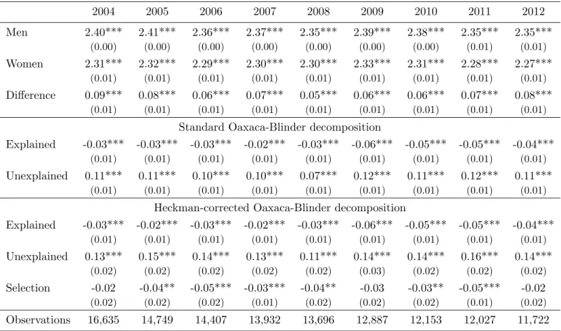
Table 3 shows the Oaxaca-Blinder decomposition of the gender wage gap for the period 2004-2012. The wage equations are presented in the Appendix (Tables A.8 and A.9). The gap in Italy is quite small compared to other European countries (Eurostat, 2015), and observable characteristics indicate that there should be a gap in favour of women. The unexplained component decreases between 2004 and 2008 and increases from 2008 to 2009. After 2009, it is large and mostly stable (between 11 percent and 12 percent).
10The most common variables used in the literature are if the parents work in the public sector, which is
not available in the data, or the number of children, which however we use already to explain participation.
11We also perform the decomposition using coefficients from the pooled regression (including both men and
women in the sample, and a dummy for sex among the control variables) or ˆβt
f as the benchmark coefficients.
Results are very similar (the unexplained component is usually larger in the last case). Available from the authors upon request.
The explained component is negative: the difference in characteristics between men and women favours women, contributing to the reduction of the gender wage gap. It increases in absolute terms between 2008 and 2009, counterbalancing the increase in the unexplained gap in this period. After 2009, the explained component decreases in absolute terms, con-tributing to the increase of the total gap. Since the explained gap is equal to the difference in characteristics by the benchmark coefficients, it may change also if the difference in char-acteristics remains stable, but the coefficients change. This is what could have happened in Italy. Working in the public sector is associated with higher wages (see Tables A.8 and A.9) and more women than men are employed in the public sector. The difference in the percentage of men and women who are public sector employees remains stable, but the return decreases in 2011 and in 2012, reducing the explained gap.
The last part of Table 3 presents the results of the decomposition taking into account self-selection (the underlying wage equations are presented in Tables A.10 and A.11). As expected, taking into account self-selection reduces the wage gap: working women in Italy are positively selected. The gap due to differences in characteristics is obviously the same as in the standard Oaxaca-Blinder decomposition. On the other hand, the term due to differences in returns is larger, partially reduced by the explained component and partially by selection. However, the overall trend is very similar to the one in the previous decomposition.
Table 3: Oaxaca-Blinder decomposition of the gender wage gap, 2004-2012 2004 2005 2006 2007 2008 2009 2010 2011 2012 Men 2.40*** 2.41*** 2.36*** 2.37*** 2.35*** 2.39*** 2.38*** 2.35*** 2.35*** (0.00) (0.00) (0.00) (0.00) (0.00) (0.00) (0.00) (0.01) (0.01) Women 2.31*** 2.32*** 2.29*** 2.30*** 2.30*** 2.33*** 2.31*** 2.28*** 2.27*** (0.01) (0.01) (0.01) (0.01) (0.01) (0.01) (0.01) (0.01) (0.01) Difference 0.09*** 0.08*** 0.06*** 0.07*** 0.05*** 0.06*** 0.06*** 0.07*** 0.08*** (0.01) (0.01) (0.01) (0.01) (0.01) (0.01) (0.01) (0.01) (0.01) Standard Oaxaca-Blinder decomposition
Explained -0.03*** -0.03*** -0.03*** -0.02*** -0.03*** -0.06*** -0.05*** -0.05*** -0.04*** (0.01) (0.01) (0.01) (0.01) (0.01) (0.01) (0.01) (0.01) (0.01) Unexplained 0.11*** 0.11*** 0.10*** 0.10*** 0.07*** 0.12*** 0.11*** 0.12*** 0.11***
(0.01) (0.01) (0.01) (0.01) (0.01) (0.01) (0.01) (0.01) (0.01) Heckman-corrected Oaxaca-Blinder decomposition
Explained -0.03*** -0.02*** -0.03*** -0.02*** -0.03*** -0.06*** -0.05*** -0.05*** -0.04*** (0.01) (0.01) (0.01) (0.01) (0.01) (0.01) (0.01) (0.01) (0.01) Unexplained 0.13*** 0.15*** 0.14*** 0.13*** 0.11*** 0.14*** 0.14*** 0.16*** 0.14*** (0.02) (0.02) (0.02) (0.02) (0.02) (0.03) (0.02) (0.02) (0.02) Selection -0.02 -0.04** -0.05*** -0.03*** -0.04** -0.03 -0.03** -0.05*** -0.02 (0.02) (0.02) (0.02) (0.01) (0.02) (0.02) (0.02) (0.01) (0.02) Observations 16,635 14,749 14,407 13,932 13,696 12,887 12,153 12,027 11,722 *p <0.1; ** p <0.05; ***p <0.01. Robust standard errors in parenthesis.
Controlling for age, experience, region of residence, marital status, level of education, sector of employment (Nace), position, part-time job, public sector. Selection equation: controlling for age, region of residence, marital status, level of education, number of children aged 0-2, 3-5, 6-10, and 11-14.
Log wages in 2008 real prices.
Benchmark coefficients: Male coefficients, shown in Table A.9 and Table A.11. Results with different bench-mark coefficients are similar (the unexplained component is larger with female coefficients as benchbench-mark). Available from the authors upon request.
4.2
Quantile decomposition
We then apply a quantile decomposition to analyse the changes of the gender pay gap at different points of the wage distribution, following the methodology proposed by Cher-nozhukov et al. (2013).
In order to extend the Oaxaca-Blinder procedures to the entire wage distribution, one needs to know the entire male, female, and counterfactual unconditional distribution of wages FW(w), for each quantile τ.
FWhm|mi represents the actual distribution of wages W for men (unconditional), and
FWhf|fi for women. FWg|Xg(w|x) is the conditional distribution of wages given the individual characteristicsXg, and FXg(x) represents the distribution of characteristics, withg ={m, f} (male and female respectively).
The counterfactual distribution of interests FWhm|fi is the unconditional distribution of wages for women if they had faced the wage structure of men12:
FWhm|fi(w) =
Z
xf
FWm|Xm(w|x)dFXf(x) (3)
The above distribution is not observed: it is constructed by integrating the conditional distribution of wages for men (FWm|Xm(w|x)) with respect to the distribution of characteristics for women (FXf(x)).
Different approaches have been proposed to estimate the counterfactual distribution. We follow Chernozhukov et al. (2013), who estimate the conditional distribution of the outcome variable FW|X using a quantile regression13 (Koenker and Bassett, 1978): QW|X(τ) =Xβτ, where QW|X(τ) =FW−1|X(τ) is the τth quantile of W conditionally on X14.
βτ is estimated by minimizing the following expression:
ˆ βτ = arg min β (1 N N X i=1 (wi−xiβ)(τ −1(wi ≤xiβ)) (4) where N is the total number of observations in the sample, and 1(·) is the indicator
12The non-discriminatory coefficients for the quantile decomposition `a la Chernozhukov et al. (2013) are
male coefficients; the counterfactual distribution shown in eq. 3 corresponds to the counterfactualXfβmin
the standard Oaxaca-Blinder decomposition, where male coefficients are used as benchmark.
13Alternatively, Chernozhukov et al. (2013) suggest to use distribution regression methods.
14Similarly, the (unconditional) quantile function is defined as the inverse of the distribution function: of Qτ(W) =FW−1(τ).
function. The covariate distribution is estimated with the empirical distribution function. The estimator for the unconditional counterfactual distribution is obtained by the plug-in-rule, integrating the estimator for conditional distribution function (estimated with quantile regression) with respect to an estimator of the covariate distribution function (estimated with the empirical distribution function). Once the counterfactual distribution has been obtained, counterfactual quantiles can be calculated by inverting the estimated distribution function.
Then, the overall difference in wages can be decomposed similarly to the traditional Oaxaca-Blinder decomposition as follows:
FYhm|mi−FYhf|fi= [FYhm|mi−FYhm|fi] + [FYhm|fi−FYhf|fi] (5) The first term is the difference due to the wage structure (or differences in returns) and the second term is the difference due to characteristics.
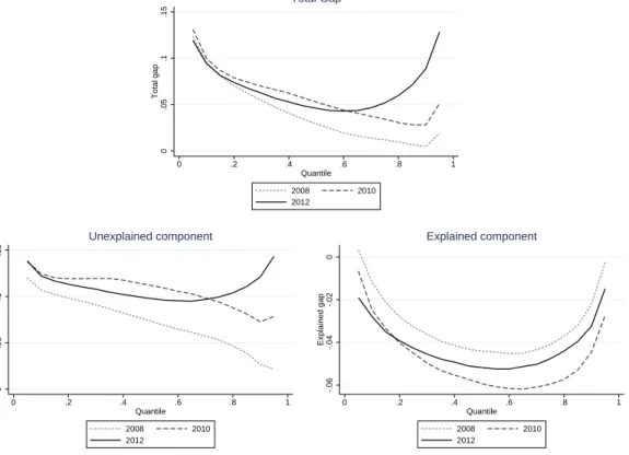
Figure 5 shows the results of the quantile decomposition. It reveals some additional features of the gender wage gap in Italy and its evolution during the crisis. In 2008, the total GWG is decreasing along the wage distribution (from 12% to 2%), with an increase only at the very top. The unexplained component accounts for more than 100%, but it is larger at the bottom of the distribution, indicating the existence of a sticky floor (Christofides et al., 2013). Both the total gender wage gap and the unexplained component widen in 2010, but their patterns along the wage distribution remain the same as in 2008. The growth of the GWG between 2008 and 2010 concerns all the working population, even though it is slightly larger for the middle and the top of the wage distribution.
In 2012 the gender wage gap has a U-shape, and it is larger at the bottom (11.9%) and at the top of the wage distribution (12.9%). The total gap is even lower than in 2010 until the 60th percentile, but it is much larger for women with wages above that threshold. In 2012, the unexplained component also increased in the upper part of the wage distribution, and has a U-shape, indicating the existence of both a sticky floor and a glass ceiling, which was not present before. Hence, the increase of the gender gap for higher-income women is partially driven by changes in their wage structure relative to men. In addition, from the 20th percentile there is an increase between 2010 and 2012 also in the explained component (i.e. due to differences in characteristics).
Figure 5: Quantile decomposition, 2008, 2010, and 2012 0 .05 .1 .15 Total gap 0 .2 .4 .6 .8 1 Quantile 2008 2010 2012 Total Gap 0 .05 .1 .15 Unexplained gap 0 .2 .4 .6 .8 1 Quantile 2008 2010 2012 Unexplained component -.06 -.04 -.02 0 Explained gap 0 .2 .4 .6 .8 1 Quantile 2008 2010 2012 Explained component
Log wages in 2008 real price. Source: EU-SILC, own calculations.
5
Impact of the wage freeze
We argue that the 2011-2012 increase of the GWG in the quantiles above 60% is a consequence of the wage freeze in the public sector. Figure 2 above shows that hourly wages in the public sector are higher than in the private sector and that wages decreased after 2010.
Looking at the estimates of the wage equations (see Tables A.7, A.8 and A.9 in the Appendix), ceteris paribus, working in the public sector is associated with higher wages: in 2010 wages in the public sector were 15% higher than in the private sector. In particular for women, until 2010, the public sector premium was more than 20%, while for men it was slightly less than 10%. Figure 6 summarizes these parameters for the pooled sample15, and
for men and women separately.
Figure 6: Public sector premium, 2004-2012 .05 .1 .15 .2 .25 Public premium 2004 2005 2006 2007 2008 2009 2010 2011 2012 Year
Pooled sample Women
Men 95% confidence bands
Parameters of public sector dummy in the wage equations. See Tables A.7, A.8, and A.9 in the Appendix.
Source: EU-SILC, own calculations.
The public sector premium decreased from 0.15 in 2010 to 0.11 in 2011 (statistically significant drop) and to 0.09 in 201216. For women, the coefficient associated with working in the public sector decreased from 0.21 to 0.15 (statistically different at 1%) between 2010 and 2011, and for men from 0.10 to 0.07 (not significant). These estimates are robust to the correction for participation into the labour market (Tables A.10 and A.11 show the Heckman-corrected results for women and men separately).
We cannot give a causal interpretation of the coefficient associated with being a woman in the pooled regression, or of those associated with the public sector variable, because of the self-selection of men and women into the public or private sector and because we cannot exclude omitted variable bias. However, they indicate that the increase in the gender wage gap was partially driven by the wage freeze. Indeed, being a woman is associated with a reduction in wages of about 10-11%, stable after 2009. On the other hand, there is an important reduction of the premium for working in the public sector in 2011, mainly for women.
5.1
Extended Oaxaca-Blinder decomposition
Having observed the discontinuity in the public sector premium, we now turn to analyse if and how it affected the gender wage gap. The law was approved in 2010 and was implemented in January 2011: thus, we compare 2009 (pre-policy period) and 2011 (post-policy period).
We first apply an extension of the Oaxaca-Blinder decomposition, which accounts for changes over time. This methodology estimates how much of the change in the gender wage gap is due to changes in individual characteristics of employed men and women, and how much can be imputed to changes in the wage structures.
The standard Oaxaca-Blinder decomposition, as shown in equation 2, is usually applied to decompose the gender wage gap in a given year between men and women. On the other hand, it can also be used to decompose the change of wages over time for a given group, as follows: ∆Wg = (lnW 11 g )−(lnW 09 g ) = (X11g −X09g ) ˆβ09 g +X 11 g ( ˆβg11−βˆg09) (6)
where g = {m, f}, 11 refers to 2011 and 09 to 2009. Since we want to isolate the changes w.r.t. 2009, we consider as benchmark coefficients ˆβ09
g 17.
The changes over time in the gender wage gap can be seen either as the difference among the GWG in 2011 and the GWG in 2009 (∆GW G = GW G11−GW G09), or as the differ-ence between changes in male wages and changes in female wages. Considering the second specification, and applying the Oaxaca-Blinder decomposition as in eq. 6, it is possible to estimate how much of the change in the gender wage gap between 2009 and 2011 is due to changes of returns (for men and for women) and how much is due to changes in individual characteristics. We call this decomposition, summarized by the following equation, ‘extended Oaxaca-Blinder decomposition’: ∆GW G= (lnW11m −lnW09m)−(lnW11f −lnW09f ) = [(X11m −X09m)βbm09 | {z } ∆ M wages due to changes in M char. + (βbm11−βbm09)X 11 m | {z } ∆ M wages due to changes in M returns ]−[(X11f −X09f )βbf09 | {z } ∆ F wages due to changes in F char. +(βbf11−βbf09)X 11 f | {z } ∆ F wages due to changes in F returns ] = (X11m −X09m)βbm09−(X 11 f −X 09 f )βbf09 | {z } ∆ GWG due to changes in characretistics + (βbm11−βbm09)X 11 m −(βbf11−βbf09)X 11 f | {z } ∆ GWG due to changes in returns (7)
We perform the ‘extended Oaxaca-Blinder’ decomposition both with and without the Heckman-correction for selection.
The aim of this decomposition is to analyse if there have been significant changes in the distribution of individual characteristics in the period around the wage freeze, which would have affected the gender wage gap. The Oaxaca-Blinder decomposition and the quantile decomposition are useful snapshots for each year, but they rely on the relative changes, exploiting the differences between male and female characteristics and between their returns. On the other hand, from the extended Oaxaca-Blinder decomposition we can isolate the changes over time in the characteristics (returns) of women, of men, and how they sum up.
For both men and women, the decrease in real (log) wages between 2009 and 2011 is entirely due to changes in the wage structures (‘∆ returns’ in Table 4). This is not surprising, considering the descriptive statistics previously shown; indeed, it would take some time to change the average characteristics of the stock of working people. As a consequence, the increase in the gender wage gap of about 1% (from 6% to 7%) can be entirely attributed to the changes in the wage structures of both men and women. Taking into account selection yields very similar results.
Table 4: Change of wages and of gender wage gap, 2009-2011 Actual wages Heckman-corrected
Men and decomposition decomposition
2011 (a) 2.35*** (0.01)
2009 (b) 2.39*** (0.00)
Change (c) -0.04*** (0.01)
Due to ∆ charact. (d) 0.01** (0.00) 0.01** (0.00) Due to ∆ return (e) -0.05*** (0.01) -0.04*** (0.01) Due to ∆ selection (f) -0.01 (0.01) Women 2011 (g) 2.28*** (0.01) 2009 (h) 2.33*** (0.01) Change (i) -0.05*** (0.01) Due to ∆ charact. (l) 0.01** (0.01) 0.01** (0.01) Due to ∆ return (m) -0.06*** (0.01) -0.07*** (0.02) Due to ∆ selection (n) 0.01 (0.02)
Gender Wage Gap
2011 (a)-(g) 0.07*** (0.01) 2009 (b)-(h) 0.06*** (0.01) ∆ GWG (c)-(i) 0.01 (0.01)
Total ∆ charact. (d)-(l) -0.00 (0.01) -0.00 (0.01) Total ∆ return (e)-(m) 0.01 (0.01) 0.03 (0.03) Total ∆ selection (f)-(n) -0.02 (0.03) * p <0.1; ** p <0.05; ***p <0.01.
Robust standard errors in parenthesis. The standard errors for the change of the Gender Wage Gap are estimated with bootstrap. Log wages in 2008 real prices.
Benchmark coefficients: 2009.
Controlling for age, experience, region of residence, marital status, level of education, sector of employment (Nace), position, part-time job, public sector. Selection equation: controlling for age, region of residence, marital status, level of education, number of children aged 0-2, 3-5, 6-10, and 11-14.
Source: EU-SILC, own calculations.
5.2
Counterfactual analysis
The previous decomposition isolates the changes in the wage structure from those in the individual characteristics, but it is not informative about the effect of the policy itself.
An additional step, to evaluate the direct impact of the wage freeze, is to estimate the counterfactual wages for men and female as if the wage freeze had never happen.
The gender wage gap at timet is: GW Gt,γt = lnW t m−lnW t f = (bδtmZ¯mt + b γtmP U BLIC¯ tm)−(bδtfZ¯ft + b γftP U BLIC¯ tf) (8) We focus only on t={2009,2011}.
We can estimate twocounterfactual gender wage gaps. The first one is the counterfactual gender wage gap in 2009, as if the public premium was the one of 2011, i.e. nothing else changed, only the return for working in the public sector:
GW G09,γ11 = lnW 09 m −lnW 09 f = (bδ09mZ¯m09+ b γm11P U BLIC¯ 09m)−(bδf09Z¯f09+ b γf11P U BLIC¯ 09f ) (9)
GW G09,γ11 can be interpreted as the gender wage gap that we would have observed with the distribution of characteristics Z of 2009, return to characteristics of 2009 (wage structure), distribution of people into the public and private sector of 2009, and public premium bγg of 201118. We interpret the public premium of 2011 as a consequence of the wage freeze in the public sector, since nothing else that could have affected it changed between 2009 and 2011. The second counterfactual is the gender wage gap in 2011, if the public premium was the one of 2009: GW G11,γ09 = lnW 11 m −lnW 11 f = (bδ11mZ¯m11+bγm09P U BLIC¯ 11 m)−(bδf11Z¯f11+bγf09P U BLIC¯ 11 f ) (10)
GW G11,γ09 is the counterfactual gender wage gap that we would have observed with the distribution of characteristics Z of 2011, return to characteristics of 2011 (wage structure), distribution of people into the public and private sector of 2011, and public premium bγg of 2009 (i.e. in the absence of the wage freeze).
Given these counterfactuals, we can decompose the change in the gender wage gap between 2009 and 2011 in a ‘policy effect’ and ‘other effects’. The ‘policy effect’ denotes the part of the gender wage gap due to changes in the public sector premium (the wage freeze in public sector). Considering the first counterfactual gender wage gap, the ‘policy effect’ corresponds
to the difference between the actual gender wage gap in 2009 (eq. 8 for 2009) and the counterfactual gender wage gap, where only the public premium has changed (eq. 9). ‘Other effects’ refer to the change in the gender wage gap due to everything else, i.e. changes in the characteristics and in the coefficients, except the public sector premium. Using the first counterfactual, it corresponds to the difference between actual gender wage gap in 2011 (eq. 8 for 2011) and the counterfactual gender wage gap (eq. 9).
Hence, considering the first counterfactual (from eq. 9), the decomposition is the following: ∆GW G=GW G11,γ11−GW G09,γ09 (total change) (11)
= (GW G11,γ11−GW G09,γ11) (other effects (1)) + (GW G09,γ11−GW G09,γ09) (policy effect (1)) In the following decomposition we employ the second counterfactual (from eq. 10):
∆GW G= (GW G11,γ11−GW G11,γ09) (policy effects (2)) (12) + (GW G11,γ09−GW G09,γ09) (other effects (2))
Finally, since there is no reason to prefer one decomposition against the other one, we cal-culate the Shapley decomposition suggested by Shorrocks (2013), and estimate the average policy effect (P) and the average effect imputed to other changes (O):
P = 1 2(GW G09,γ11−GW G09,γ09) + 1 2(GW G11,γ11 −GW G11,γ09) (13) O= 1 2(GW G11,γ11−GW G09,γ11) + 1 2(GW G11,γ09 −GW G09,γ09)
This analysis is also replicated taking into account selection. In this case, GW G09,γ09 and
GW G11,γ11 represent the gender wage gaps estimated for 2009 and in 2011 using the predicted wages with Heckman-corrections. Similarly, the corrected coefficients are used to estimate the counterfactual wage gaps in equations 9 and 10.
Table 5 and 6 show, respectively, the counterfactual simulation - which allows us to isolate the impact of the wage freeze - and the related decomposition into ‘policy effect’ and ‘other effects’.
Table 5: Actual and counterfactual gender wage gaps, 2009 and 2011 Heckman-corrected Gender Wage Gaps Obs. Mean S.E. Mean S.E.
GW G09,γ09 12,887 0.06*** (0.01) 0.09*** (0.00)
GW G11,γ11 12,027 0.07*** (0.01) 0.11*** (0.01)††
Counterfactual Gender Wage Gaps
GW G09,γ11 12,887 0.08*** (0.01)†† 0.11*** (0.00)††
GW G11,γ09 12,027 0.05*** (0.01)† 0.10*** (0.01)†
* p <0.1; **p <0.05; *** p <0.01;
† sig. different fromGW G11,γ11 (p <0.05);
††sig. different fromGW G09,γ09 (p <0.01).
Robust standard errors in parenthesis; for Heckman GWG and the counter-facutal GWG bootstrapped standard errors in parenthesis.
Source: EU-SILC, own calculations.
Tables 5 presents the actual wage gaps in 2009 (6%) and in 2011 (7%), and the estimations of two counterfactuals, constructed as discussed above. GW G09,γ11 is the gender wage gap that we would have observed in 2009 if the coefficient associated for working in the public sector was the same of 2011: GW G09,γ11 is estimated to be 8% (Table 5), larger and signifi-cantly different (at 1%) from GW G09,γ09, the actual gender wage gap in 2009. Since we keep constant the individual characteristics, the rest of the wage structure, and the proportion of people working in the public sector, the difference of 2% among the two wage gaps is entirely due to the wage freeze (Table 6).
The second counterfactual, GW G11,γ09, represents the gender wage gap that we would have measured in 2011 with the public sector premium of 2009,everything else equal to 2011 values. It is estimated at 5.1%, significantly smaller than the actual gender gap in 2011.
Hence, even though the change between 2009 and 2011 is small, it is completely due to the changes in the return to the public sector - which we can interpret as the consequence of the wage freeze introduced by the government, partially compensated by other changes (Table 6). Moreover, an increase of 1 percentage point on a gender wage gap of about 6-8% is important, in particular when considering that the increase continued in 2012, and probably in the following years.
Table 6: Decomposing the change in the gender wage gap, 2009-2011
Heckman-corrected Total change GW G11,γ11 - GW G09,γ09 0.01 (0.01) 0.03*** (0.01)
Diff. due to the policy (1) GW G09,γ11 - GW G09,γ09 0.02*** (0.01) 0.02*** (0.00)
Diff. due to the policy (2) GW G11,γ11 - GW G11,γ09 0.02*** (0.01) 0.02*** (0.00)
Diff. due to other changes (1) GW G11,γ11 - GW G09,γ11 -0.01 (0.01) 0.01 (0.01)
Diff. due to other changes (2) GW G11,γ09 - GW G09,γ09 -0.01* (0.01) 0.01 (0.01)
Shorrocks-Shapley decomposition
Average diff. due to the policy 0.02*** (0.00) 0.02*** (0.00) Average diff. due to other changes -0.01 (0.01) 0.01 (0.01)
*p <0.1; **p <0.05; ***p <0.01.
Bootstrapped standard errors in parenthesis. Source: EU-SILC, own calculations.
The last two columns of Table 5 present the gender wage gaps predicted using the Heckman-corrected coefficients. As expected, they are larger then the observed ones, and they increase from 2009 (8.7%) to 2011 (11.5%).
The Heckman-corrected counterfactualGW G09,γ11 (10.6%) is significantly larger than the gender wage gap in 2009, while GW G11,γ09 (10.7%) is significantly smaller than the gender wage gap in 2011.
As one could expect, since the estimated public sector premium is the same with and without Heckman correction, the difference due to the policy is the same (2%). However, the total difference is larger when selection is taken into account (2.7%), and ‘other changes’ also slightly contribute to it (in particular, in this case, they are the changes due to the returns associated with other explanatory variables).
When we estimate the counterfactuals, we make use of the public sector premium in 2009 and in 2011 to isolate the impact of the wage freeze on the gender wage gap. This relies on the assumption that between 2009 and 2011 nothing else changed, which could affect the public sector premium. It seems a realistic assumption since there was no other policy change. The proportion of people working in the public sector did not change and the stock of working people was similar in the two periods. Hence, we can consider that the counterfactual analysis isolates the impact of the wage freeze on the gender wage gap.
On the other hand, we cannot claim that in the absence of such a policy everything else would have been as it is in 2011. The wage freeze was justified as one of the way to reduce public spending and improve the conditions of Italian economy. One could claim that the government could have taken other measures instead of the wage freeze. Plausibly, that would have caused other changes on employment and on the wage structure - no matter if the policy would have been in the direction of cutting public spending (as the wage freeze) or in the opposite direction. We follow here a partial equilibrium approach, as it is usually the case with decomposition and counterfactual methodologies, thus we cannot derive general equilibrium considerations (Fortin et al., 2011).
6
Within public sector
In the previous section, we have shown that the gender wage gap increased due to the public sector wage freeze. This increase could be due to the large proportion of women employed in the public sector. If that was the only mechanism in place, we would expect a stable gender wage gap within the public sector.
Thus, as a final contribution, we analyse changes within the public sector. We first compute the gender wage gap separately for the public and the private sector, presented in Figure 7. The gender wage gap in the public sector is always smaller than in the private one. It decreased in 2006, remained not significantly different from 0 until 2010 and then it increased sharply reaching 5.9% in 2011 and 6.6% in 2012. The GWG within the private sector slightly decreases over time.
Hence, the gender wage gap in the public sector is not stable as one might have ex-pected. Considering the different distribution of men and women in the public sectors (see section 3), we investigate if this gap emerged as a consequence of the sector-specific policy implementation (see section 2). More than 75% of employees in education are women.
Looking at the trend in wages in the different public sectors, we note that in the education sector average hourly wages decreased more than in other sectors (see Figure 8). Wages de-creased by 15.6% in 2011 for women and by 11.7% for men (see Table A.12 in the Appendix). In addition, female wages decreased more than male ones in education, public administration, and health sectors. The sector ‘others’ is a residual group that we do not compare with the previous mentioned sectors, because it could include heterogeneous categories by gender.
In order to control for other covariates, we estimate three wage equations for men, women, and the pooled sample employed in the public sector. In addition to the usual controls
Figure 7: Gender wage gap, public and private sector, 2004-2012 -5 0 5 10 15 20 Gap 2004 2005 2006 2007 2008 2009 2010 2011 2012 Public sector Private sector 95% confidence bands
Gross wages per hour in 2008 real price. Source: EU-SILC, own calculations.
Figure 8: Wages in the public sector, by gender and sub-sector of employment, 2004-2012
13 14 15 16 17 18 2004 2005 2006 2007 2008 2009 2010 2011 2012 Year Women Men Education 12 12.5 13 13.5 14 2004 2005 2006 2007 2008 2009 2010 2011 2012 Year Women Men Public Administration 12 14 16 18 2004 2005 2006 2007 2008 2009 2010 2011 2012 Year Women Men Health 11 11.5 12 12.5 13 13.5 2004 2005 2006 2007 2008 2009 2010 2011 2012 Year Women Men Other sectors
Gross wages per hour in 2008 real price. Source: EU-SILC, own calculations.
(age, education, region, marital status, experience, position), we control for the following sub-sectors: Public administration and Defence, Education, Health, and Other sectors (see Tables A.13, A.14, and A.15).
Before 2010, working in the (public) education sector had a positive impact on wages compared to other public sectors, especially for women19 However, the premium dropped from 8% in 2010 to 0% in 2011 and 2012. The decrease is particularly remarkable for women, for whom the coefficient associated with working in education dropped from 11% in 2010 to 1% in 2011. For men, this coefficient decreased from 0% in 2010 to -4% in 2011.
Therefore, we can conclude that the abolition of the automatic seniority wage increases in the public education sector (due to the 2010 law) contributed to the increase of the gender wage gap within the public sector. It could be interesting to analyse in details the increase of the gender wage gap in different public sectors, but unfortunately the small number of observations and the type of data do not allow a deeper investigation.
7
Conclusions
Despite the Italian gender gap being much lower than the European average, and despite some studies showing that the great recession in Italy had a less negative impact on women than on men, the gender pay gap increased from 4% to 8% between 2008 and 2012.
We show that the Italian gender wage gap is completely unexplained by observed char-acteristics, applying the Oaxaca-Blinder decomposition to EU-SILC data. The quantile de-composition shows two different trends before and after 2010. Between 2008 and 2010, the gender pay gap increased along the entire quantile distribution both in the explained and unexplained components. After 2010, the gender wage gap increased largely among people in the upper part of the wage distribution.
We argue that the 2011-2012 increase of the gender wage gap in the quantiles above 60% is a consequence of the wage freeze in the public sector, introduced as an austerity measure during the economic crisis.
The application of a counterfactual analysis shows that more than 100% (about 70% when we account for selection) of the GWG growth between 2009 and 2011 is due to the wage freeze in the public sector: it reduced the public sector premium and had a disproportionate impact on women.
This is not only due to the large proportion of women working in the public sector, but also to the larger wage drop in the public education sector, where about 75% of the employees are women.
We might expect a further increase in the gender wage gap for the period 2012-2015, since the wage freeze has been extended until mid 2015. In June 2015, the Italian Constitutional Court declared that the public sector wage freeze is not legitimate. The decision will affect only the future wage bargaining, but it will not compensate for the previous losses (January 2011- June 2015).
Economic policies regarding public sector pay freezes and cuts in the service sector, imple-mented during this crisis, have serious gender side effects, that have often been disregarded. Similar policies have been introduced also in other European countries (Estonia, Greece, Hun-gry, Ireland, Latvia, Lithuania, Portugal, Czech Republic, Romania, Spain) (EPSU, 2012) and it would be interesting to estimate their effects comparing short term policies (e.g. wage cuts for one year) with medium term ones (e.g. wage freeze for several years). Possible future developments of this paper, with a larger sample, include a deeper analysis of the changes within the public sector, together with a detailed analysis of the wages within the public education sector.
References
Addabbo, T., Favaro, D., 2011. Gender wage differentials by education in Italy. Applied Economics 43(29), 4589–4605.
Bettio, F., 2013. Perch´e in Italia si riapre il gender pay gap. http://www.ingenere.it/ articoli/perch-italia-si-riapre-il-gender-pay-gap.
Bettio, F., Corsi, M., D’Ippoliti, C., Lyberaki, A., Lodovici, M. S., Verashchagina, A., 2013. The impact of the economic crisis on the situation of women and men and on gender equality policies. Synthesis report, European Commission.
Blinder, A. S., 1973. Wage Discrimination: Reduced Form and Structural Estimates. Journal of Human Resources 8(4), 436–455.
Bordogna, L., 2013. Employment relations and union action in the Italian public services: Is there a case of distortion of democracy? Comparative Labor Law & Policy Journal 34(2), 507–530.
Bordogna, L., Neri, S., 2012. Social dialogue and the public services in the aftermath of the economic crisis: strengthening partnership in an era of austerity in Italy. National report VP/2011/001, European Commission project, Industrial Relations and Social Dialogue. Bredtmann, J., Otten, S., Rulff, C., 2014. Husband’s Unemployment and Wife’s Labor
Sup-ply? The Added Worker Effect across Europe. Ruhr Economic Papers 484.
Chernozhukov, V., Fern´andez-Val, I., Melly, B., 2013. Inference on counterfactual distribu-tions. Econometrica 81(6), 2205–2268.
Christofides, L. N., Polycarpou, A., Vrachimis, K., 2013. Gender wage gaps, ‘sticky floors’ and ‘glass ceilings’ in Europe. Labour Economics 21, 86–102.
Del Bono, E., Vuri, D., 2011. Job mobility and the gender wage gap in Italy. Labour Eco-nomics 18(1), 130–142.
Depalo, D., Giordano, R., Papapetrou, E., 2015. Public-private wage differentials in euro-area countries: evidence from quantile decomposition analysis. Empirical Economics Online first http://dx.doi.org/10.1007/s00181-014-0900-0.
EPSU, 2012. The wrong target one year on: pay cuts in the public sector in the European Union. Technical report, Labour Research Department.
European Commission, 2015. Special Eurobarometer 428 “Gender Equality”. Report, Euro-pean Union, Brussels.
Eurostat, 2015. Sustainable development indicators: social inclusion. Gender pay gap in unadjusted form. http://ec.europa.eu/eurostat/tgm/table.do?tab=table&init=1& language=en&pcode=tsdsc340&plugin=1.
Figari, F., Fiorio, C., 2015. Fiscal consolidation policies in the context of Italy’s two reces-sions. Euromod Working Paper EM 7/15.
Fortin, N., Lemieux, T., Firpo, S., 2011. Chapter 1 - Decomposition Methods in Economics.
Handbook of Labor Economics, volume 4, Part A, pp. 1–102, Elsevier.
Ghignoni, E., Verashchagina, A., 2014. Can the crisis be an opportunity for women? In: Malo, M. A., Sciulli, D. (Eds.), Disadvantaged Workers, AIEL Series in Labour Economics, pp. 257–276, Springer International Publishing, Cham.
Heckman, J., 1974. Shadow prices, market wages, and labor supply. Econometrica 42(4), 679–694.
Istat, 2010. La divisione dei ruoli nelle coppie, Famiglia e Societ`a. http://www3.istat.it/ salastampa/comunicati/non_calendario/20101110_00/testointegrale20101110. pdf.
Istat, 2015. Occupati e disoccupati, Serie storiche. http://www.istat.it/it/archivio/ 167286.
Koenker, R., Bassett, G. J., 1978. Regression Quantiles. Econometrica 46(1), 33–50.
Mussida, C., Picchio, M., 2014a. The gender wage gap by education in Italy. The Journal of Economic Inequality 12(1), 117–147.
Mussida, C., Picchio, M., 2014b. The trend over time of the gender wage gap in Italy. Empirical Economics 46(3), 1081–1110.
Neuman, S., Oaxaca, R. L., 2004. Gender versus Ethnic Wage Differentials among Profes-sionals: Evidence from Israel. Annales d’´Economie et de Statistique (71/72), 267–292. Nicodemo, C., 2009. Gender pay gap and quantile regression in European families. IZA
Discussion Paper 3978.
Oaxaca, R., 1973. Male-female wage differentials in urban labor markets. International Eco-nomic Review 14(3), 693–709.
OECD, 2009. Society at a glance: OECD Social Indicators. Technical report, OECD, Paris. Olivetti, C., Petrongolo, B., 2008. Unequal Pay or Unequal Employment? A Cross-Country
Analysis of Gender Gaps. Journal of Labor Economics 26(4), 621–654.
Piazzalunga, D., 2015. Is there a Double-Negative Effect? Gender and Ethnic Wage Differ-entials in Italy. LABOUR: Review of Labour Economics and Industrial Relations, 29(3), 243–269.
Shorrocks, A. F., 2013. Decomposition procedures for distributional analysis: a unified frame-work based on the Shapley value. The Journal of Economic Inequality 11(1), 99–126.
Sierminska, E., Takhtamanova, Y., 2011. Job Flows, Demographics, and the Great Reces-sion. In: Immervoll, H., Peichl, A., Tatsiramos, K. (Eds.), Who Loses in the Downturn? Economic Crisis, Employment and Income Distribution (Research in Labor Economics, Volume 32), pp. 115–154, Emerald Group Publishing Limited.
Tronti, L., 2011. Regulating wages and collective bargaining in the public sector. Technical report, Presidenza del Consiglio dei Ministri, Dipartimento della Funzione Pubblica. Villa, P., Smith, M., 2010. Gender Equality, Employment Policies and the Crisis in EU
A
Appendix
T able A.1: Sample selection Initial sample Only Italian 20-65 No retired No unempl. No inactiv e Only emplo y ees No missing w age Final Sample 52,608 51,294 37,523 33,398 30,927 22,36 2 16,641 16,635 47,899 46,747 33,916 30,400 28,183 20,48 0 14,798 14,749 46,522 45,365 32,519 29,195 27,070 19,71 8 14,441 14,407 45,133 43,617 31,077 27,977 26,090 19,05 8 13,967 13,932 44,805 43,187 30,502 27,593 25,636 18,76 5 13,724 13,696 43,636 41,974 29,509 26,733 24,567 17,96 1 12,910 12,887 40,836 38,754 27,547 25,146 22,981 16,78 5 12,178 12,153 40,496 38,862 27,644 25,003 22,603 17,00 7 12,055 12,027 40,287 38,579 27,267 24,843 22,283 16,42 5 11,754 11,722 402,222 388,379 277,504 250,288 230,340 168,561 122,468 122,208 EU-SILC, o wn calculations.Table A.2: Variables description
Variable Description
Women Dummy variable. 1 if woman, 0 otherwise.
Monthly wage Gross monthly earnings for employees, before tax and contribution, in euro. It includes usual paid overtime, tips and commissions in euro (py200g). Reference period: year of the survey. Wages in 2008 real prices.
Hours per week Number of hours usually worked per week, including usual extra hours (pl060). Reference period: year of the survey.
Hourly wage Monthly wage divided by hours per week times 4.3. Log hourly wage Natural log of hourly wage.
Age Year of interview - year of birth (rb080).
Experience Number of years spent in paid work from the first job (maternity leave included) (pl200). Self-defined.
Public sectora Dummy variable. 1 if working in the public sector, 0 otherwise. Self-defined. Avail-able in the Italian sample (variAvail-able SETTOR).
Part-time Dummy variable. 1 if working part-time (pl031). Self-defined. Region
North Dummy variable. 1 if living in: Aosta Valley, Piedmont, Liguria, Lombardy, Trentino-Alto Adige, Veneto, Friuli-Venezia Giulia, Emilia Romagna, 0 otherwise. Centre Dummy variable. 1 if living in: Tuscany, Umbria, Marche, Lazio, 0 otherwise. South Dummy variable. 1 if living in: Abruzzo, Molise, Campania, Apulia, Basilicata,
Calabria, Sicilia, Sardegna, 0 otherwise. Education Highest ISCED level attained (pe040):
Primary Dummy variable. 1 if no education, pre-primary education or primary education (ISCED 0 and ISCED 1), 0 otherwise.
Lower secondary Dummy variable. 1 if lower secondary education (ISCED 2), 0 otherwise. Upper secondary Dummy variable. 1 if upper secondary education (ISCED 3), 0 otherwise.
Post-secondary Dummy variable. 1 if post-secondary non tertiary education (ISCED 4), 0 otherwise. Tertiary Dummy variable. 1 if first or second stage of tertiary education (ISCED 5 and
ISCED 6), 0 otherwise. Marital status
Married Dummy variable. 1 if married (pb190=1) and she/he is not in consensual union without a legal basis (pb2006=2), 0 otherwise.
Cohabiting Dummy variable. 1 if in consensual union without a legal basis (pb200=2), 0 oth-erwise.
Other Dummy variable. 1 if single, separated, divorced, widowed ((pb1906=1) and not in consensual union without a legal basis (pb2006=2), 0 otherwise.
Sector (Nace)b,c The economic activity of the local unit of the main job for respondents at work: NACE rev.1.1 until 2008 (pl110); NACE rev.2 since 2011 (pl111).
Agriculture Dummy variable. 1 if NACE=1 to 5 (agriculture, hunting, forestry, fishing), 0 otherwise.
Manufacture Dummy variable. 1 if NACE =10 to 41 (mining and quarrying, manufacturing, electricity, gas and water supply; waste management), 0 otherwise.
Construction Dummy variable. 1 if NACE =45 (construction), 0 otherwise.
Table A.2: (continued)
Variable Description
Commerce Dummy variable.1 if NACE =50 to 64 (Wholesale and retail trade; repair of motor vehicles, motorcycles and personal and household goods; hotels and restaurants; transport, storage and communication), 0 otherwise.
Services Dummy variable. 1 if NACE =65 to 99 (Financial intermediation; real estate, renting and business activity, public administration and defence, compulsory social security; education; health and social work; other community, social and personal service activities; private households with employed persons; extra-territorial organizations and bodies), 0 otherwise. In 2011 the definition for these categories are slightly different, but this main group covers the same as in 2008.
Positionb Using the variable posdip (available in the Italian sample).
Managers Dummy variable. 1 if manager, 0 otherwise. Supervisors Dummy variable. 1 if supervisor, 0 otherwise.
White collar Dummy variable. 1 if employee/clerical worker, 0 otherwise.
Blue collar Dummy variable. 1 if workman, apprentice, or working from home for a company, 0 otherwise.
Children These variables use mother id (rb230), father id (rb240) and age.
Children 0-2 Dummy variable. 1 if she/he has children aged 0-2, 0 otherwise. Children 3-5 Dummy variable. 1 if she/he has children aged 3-5, 0 otherwise. Children 6-10 Dummy variable. 1 if she/he has children aged 6-10, 0 otherwise. Children 11-14 Dummy variable. 1 if she/he has children aged 11-14, 0 otherwise.
a To determine if the individual works in the public or in the private sector, we rely on individuals’ replies (while this information is not available in the standard EU-SILC, it is an additional variable provided in the Italian sample). Cross-checking with the Nace classification is entirely reassuring: on average, more than 30% of people in the public sector work in Public administration and defence, about 30% in Education and 20% in Health and social work (See Table A.5 and A.6, respectively for women and for men).
b Both the Nace and the Isco classification changed during the period covered by our paper (2004-2012). While the new Nace classification, used since 2009, is very similar to the old one, and we can switch from one to the other one without any problem, this is not the case for the Isco classification. Some major changes where introduced since 2011 and the new classification is not entirely comparable with the old one. To avoid misinterpretation, we control for the position, instead of the type of occupation, which provides similar information.
c With respect to the Nace classification, when considering the full sample we aggregated the different sectors into Agriculture, Manufacture, Construction, Commerce and Services. For the analysis within the public sector, however, we aggregated the same sectors into Public administration and defence, Education, Health and social work, Other sectors. In fact, even though there are people employed in every sub-sector even within the public sector, the percentage of those employed in sectors different than those just listed is too small to perform a good analysis, in particular for women.
Table A.3: Descriptive statistics - Employed and non-working Italian women (20-65 yo), 2004-2012 2004 2005 2006 2007 2008 2009 2010 2011 2012 Age 42.48 42.65 42.87 43.07 43.33 43.33 43.52 44.33 44.54 North 0.46 0.45 0.44 0.43 0.43 0.43 0.42 0.44 0.45 Centre 0.24 0.23 0.23 0.23 0.23 0.22 0.22 0.23 0.24 South 0.30 0.32 0.33 0.34 0.34 0.35 0.37 0.33 0.32 Married 0.61 0.61 0.61 0.61 0.60 0.59 0.58 0.59 0.58 Cohabiting 0.03 0.04 0.04 0.04 0.04 0.04 0.05 0.05 0.05 Other marital st. 0.37 0.36 0.35 0.36 0.36 0.37 0.37 0.36 0.37 Primary 0.21 0.20 0.17 0.15 0.14 0.13 0.13 0.12 0.10 Lower secondary 0.28 0.27 0.27 0.28 0.27 0.27 0.27 0.27 0.26 Upper secondary 0.36 0.36 0.36 0.37 0.41 0.41 0.40 0.41 0.43 Post-secondary 0.05 0.07 0.08 0.08 0.05 0.05 0.05 0.04 0.04 Tertiary 0.11 0.11 0.12 0.12 0.13 0.14 0.15 0.16 0.17 Children 0-2 0.07 0.07 0.07 0.07 0.06 0.06 0.05 0.06 0.05 Children 3-5 0.08 0.07 0.07 0.07 0.07 0.08 0.08 0.07 0.07 Children 6-10 0.12 0.12 0.13 0.12 0.12 0.13 0.12 0.12 0.12 Children 11-14 0.11 0.11 0.11 0.11 0.11 0.11 0.11 0.11 0.11 Observations 16,341 14,401 13,875 13,426 13,220 12,689 11,848 11,437 11,280
Source: EU-SILC, own calculations.
Table A.4: Descriptive statistics - Employed and non-working Italian men (20-65 yo), 2004-2012 2004 2005 2006 2007 2008 2009 2010 2011 2012 Age 41.92 42.14 42.21 42.45 42.53 42.74 42.79 43.54 43.61 North 0.46 0.45 0.45 0.44 0.43 0.44 0.43 0.45 0.45 Centre 0.24 0.23 0.23 0.23 0.23 0.23 0.22 0.24 0.24 South 0.30 0.32 0.33 0.33 0.34 0.33 0.35 0.32 0.31 Married 0.56 0.56 0.56 0.55 0.54 0.54 0.53 0.55 0.53 Cohabiting 0.03 0.04 0.04 0.04 0.04 0.04 0.05 0.05 0.05 Other marital st. 0.42 0.40 0.41 0.41 0.42 0.42 0.43 0.41 0.42 Primary 0.16 0.15 0.12 0.11 0.11 0.09 0.09 0.08 0.08 Lower secondary 0.34 0.32 0.32 0.32 0.31 0.32 0.32 0.32 0.31 Upper secondary 0.37 0.38 0.39 0.39 0.43 0.43 0.44 0.45 0.46 Post-secondary 0.04 0.05 0.07 0.07 0.04 0.04 0.04 0.02 0.03 Tertiary 0.10 0.10 0.10 0.11 0.11 0.12 0.12 0.13 0.13 Children 0-2 0.06 0.06 0.06 0.06 0.06 0.06 0.05 0.06 0.05 Children 3-5 0.07 0.07 0.07 0.07 0.07 0.07 0.07 0.07 0.06 Children 6-10 0.11 0.11 0.12 0.12 0.12 0.12 0.12 0.11 0.11 Children 11-14 0.10 0.10 0.10 0.10 0.10 0.10 0.09 0.10 0.10 Observations 14,133 12,366 11,898 11,383 11,161 10,650 10,077 9,726 9,704