Full Terms & Conditions of access and use can be found at
https://www.tandfonline.com/action/journalInformation?journalCode=tcfm20
Engineering Applications of Computational Fluid
Mechanics
ISSN: 1994-2060 (Print) 1997-003X (Online) Journal homepage: https://www.tandfonline.com/loi/tcfm20
Comparative analysis of soft computing
techniques RBF, MLP, and ANFIS with MLR and
MNLR for predicting grade-control scour hole
geometry
Hossien Riahi-Madvar, Majid Dehghani, Akram Seifi, Ely Salwana,
Shahaboddin Shamshirband, Amir Mosavi & Kwok-wing Chau
To cite this article: Hossien Riahi-Madvar, Majid Dehghani, Akram Seifi, Ely Salwana,Shahaboddin Shamshirband, Amir Mosavi & Kwok-wing Chau (2019) Comparative analysis of soft computing techniques RBF, MLP, and ANFIS with MLR and MNLR for predicting grade-control scour hole geometry, Engineering Applications of Computational Fluid Mechanics, 13:1, 529-550, DOI: 10.1080/19942060.2019.1618396
To link to this article: https://doi.org/10.1080/19942060.2019.1618396
© 2019 The Author(s). Published by Informa UK Limited, trading as Taylor & Francis Group
Published online: 22 Jun 2019.
Submit your article to this journal
Article views: 88
2019, VOL. 13, NO. 1, 529–550
https://doi.org/10.1080/19942060.2019.1618396
Comparative analysis of soft computing techniques RBF, MLP, and ANFIS with
MLR and MNLR for predicting grade-control scour hole geometry
Hossien Riahi-Madvara, Majid Dehghanib, Akram Seifia, Ely Salwanac, Shahaboddin Shamshirbandd,e, Amir Mosavif,gand Kwok-wing Chauh
aDepartment of Water Science & Engineering, Faculty of Agriculture, Vali-e-Asr University of Rafsanjan, Rafsanjan, Iran;bTechnical and
Engineering Department, Faculty of Civil Engineering, Vali-e-Asr University of Rafsanjan, Rafsanjan, Iran;cInstitute of Visual Informatics,
Universiti Kebangsaan Malaysia, Malaysia;dDepartment for Management of Science and Technology Development, Ton Duc Thang University, Ho Chi Minh City, Vietnam;eFaculty of Information Technology, Ton Duc Thang University, Ho Chi Minh City, Vietnam;fInstitute of Automation, Kando Kalman Faculty of Electrical Engineering, Obuda University, Budapest-, Hungary;gSchool of the Built Environment, Oxford Brookes University, Oxford, UK;hDepartment of Civil and Environmental Engineering, Hong Kong Polytechnic University, Hong Kong, People’s Republic
of China ABSTRACT
The main aims and contributions of the present paper are to use new soft computing methods for the simulation of scour geometry (depth/height and locations) in a comparative framework. Five models were used for the prediction of the dimension and location of the scour pit. The five developed mod-els in this study are multilayer perceptron (MLP) neural network, radial basis functions (RBF) neural network, adaptive neuro fuzzy inference systems (ANFIS), multiple linear regression (MLR), and mul-tiple non-linear regression (MNLR) in comparison with empirical equations. Four non-dimensional geometry parameters of scour hole shape are predicted by these models including the maximum scour depth (S), the distance of S from the weir (XS), the maximum height of downstream deposited sediments (hd), and distance of hd from the weir (XD). The best results over train data derived for XS/Z and hd/Z by the MLP model with R2are 0.95 and 0.96 respectively; the best predictions for S/Z and XD/Z are from the ANFIS model with R20.91 and 0.96 respectively. The results indicate that the application of MLP and ANFIS results in the accurate prediction of scour geometry for the designing of stable grade control structures in alluvial irrigation channels.
ARTICLE HISTORY
Received 1 February 2019 Accepted 9 May 2019
KEYWORDS
scour geometry; alluvial channels; artificial intelligence; grade control structure; big data; radial basis functions
1. Introduction
Grade control structures are commonly used in irrigation channels for regulating water level, supplying required head upstream of weirs, measuring flow rate, enhancing water quality by reducing erosion, and preventing degra-dation in a bed channel of alluvial materials (Najafzadeh,
2015). The performance of the irrigation channel will increase by using these structures. Water flowing from the top crest of the weir (as one of the grade control structures) creates a vortex and increases flow veloc-ity downstream of hydraulic structures that result in local scour (Mohammadpour,2017; Sarkar & Dey,2004). Local scour creates holes downstream of a weir and its dimensions increase gradually and become unbalanced, which causes the failure of the hydraulic structures or weir (Goel & Pal, 2009). Therefore, it is necessary that adequate effort and attention are given to the safe design of the foundations of hydraulic structures (Sarkar & Dey,
CONTACT Shahaboddin Shamshirband [email protected] Department for Management of Science and Technology Development, Ton Duc Thang University, Ho Chi Minh City, Vietnam
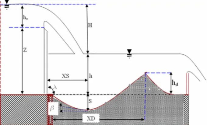
2004; Termini & Sammartano,2012). There are various hydraulic and geotechnical factors that have an effect on the local scour downstream of water level adjust-ing structures in erodible beds. Figure 1shows a plan view of local scour on an alluvial bed downstream of a water level control structure at the equilibrium stage (D’Agostino & Ferro, 2004). Local sediment transport is actively done throughout the developing stage of the local scour pit. With approaching the equilibrium state, this phenomenon becomes a ‘purely hydraulic’ mecha-nism, where mass balance among removed and deposited particles at the downstream creates the scour hole pro-file (D’Agostino & Ferro, 2004). Generally, the scour around the level control structures is essentially complex progress because of the three-dimensional flow patterns relating to alluvial bed materials and erodible beds. In conjunction with Figure1, it is clear that the four geomet-ric parameters that define the local scour hole dimensions
© 2019 The Author(s). Published by Informa UK Limited, trading as Taylor & Francis Group
This is an Open Access article distributed under the terms of the Creative Commons Attribution License (http://creativecommons.org/licenses/by/4.0/), which permits unrestricted use, distribution, and reproduction in any medium, provided the original work is properly cited.
Figure 1.Schematic view of scour geometry downstream of grade control structures.
and geometry are: maximum scour depth (S); distance of S from the weir (XS); maximum height of downstream deposited sediments (hd); and distance of hd from the
weir (XD). An accurate estimation of these four scour hole dimensions around the water level adjusting struc-tures is one of the most important stages in grade con-trol structure design and is the main contribution of the present study.
The scour mechanism for grade control structures is complex and is usually studied by regression anal-ysis or simple empirical equations. Various investiga-tors have widely studied the local scour process around the water level control structures based on experimental and prototype observations (Guan, Melville, & Friedrich,
2016; Lenzi, Marion, Comiti, & Gaudio,2002; Lu, Hong, Chang, & Lu, 2013; Marion, Tregnaghi, & Tait, 2006; Pagliara & Kurdistani,2013; Scurlock, Thornton, & Abt,
2011). Mason and Arumugam (1985) and Hoffmans and Verheij (1997) proposed many regression equations for estimating the final scour depth. Gaudio, Marion, and Bovolin (2000) presented an equation to predict the depth and length of a scour pit by using sediment par-ticle size and morphological length. Lenzi, Marion, and Comiti (2003) investigated many water level adjustment structures in mountain rivers to assess the effects of a water flow jet on the progress of scouring. Pagliara (2007) developed a regression equation to characterize the scour pit shape. Kumar and Sreeja (2012) investigated the scour depth prediction by several experimental equations pre-sented in the literature by using experimental and field data. In regard to these results, it is concluded that the predictive equations for scour depth cannot be used gen-erally for all ranges of total water head and flow discharge. Melville and Lim (2014) collected some laboratory data and developed a formula to estimate the scour dimension for a horizontal 2D jet. Rajaei, Esmaeili Varaki, and Shafei Sabet (2019) studied the influences of various factors on
local scour downward of water level adjusting structures in trapezoidal and rectangular labyrinth plan form.
Prediction of local scour hole geometry is a major and critical subject in water resource engineering for prevent-ing excessive channel bed degradation and protectprevent-ing the stability of water level adjustment structures (Lau-celli & Giustolisi,2011) in alluvial channels. The scour process around the level adjustment structures can dam-age these structures and downstream channel geometry (Najafzadeh, 2015). Traditional and statistical methods such as regression methods are limited to the studies in the experimental and field conditions. Sometimes, this concern dose not lead to providing the accurate prediction for scour depth. Consequently, the equations that are extended based on these methods cannot be applicable in most cases (Hooshyaripor, Tahershamsi, & Golian,2014). Hence, developing new techniques for modifying traditional physical-based analysis is crucial. Recently, using artificial soft computing models such as artificial neural network (ANN) simulation models and a fuzzy based model, adaptive neuro fuzzy infer-ence system (ANFIS) has been introduced as an accu-rate learning scheme for modeling complex phenomena in different aspects of hydraulic and water engineering problems (Bateni & Jeng, 2007; Chau, 2017; Hameed et al.,2017; Moazenzadeh, Mohammadi, Shamshirband, & Chau,2018; Taormina, Chau, & Sivakumar,2015; Wan Mohtar, Afan, El-Shafie, Bong, & Ab. Ghani,2018; Wu & Chau, 2011; Yaseen, El-Shafie, Afan, Hameed, Wan Mohtar & Hussain,2016; Yaseen, Sulaiman, Deo, & Chau,
2019; Zounemat-Kermani, Beheshti, Ataie-Ashtiani, & Sabbagh-Yazdi,2009). These artificial intelligence meth-ods benefit from the simplicity, ability, and proper results of modern and advanced computers (Nguyen, Ahn, & Park, 2018; Salmasi, Yıldırım, Masoodi, & Parsamehr,
2013), knowledge based and data based nature, predic-tions without need of model form, and greater endurance over the data errors (Azamathulla,2005; Bateni & Jeng,
2007) than statistical models. For instance, Liriano and Day (2001) reported higher performance of the ANN method in estimating scour dimension near a culvert in comparison to the existing empirical equations. Goel and Pal (2009) compared the results of support vec-tor machines (SVM) and ANN models with an empir-ical equation for modeling scour. Based on the results, the SVM model showed better performance than both ANN and empirical equations for scour prediction. Aza-mathulla (2012) studied a gene-expression programming (GEP) model for estimating scour depth at the down-stream of sills and the results compared to estimations of existing equations in Chinnarasri and Kositgittiwong (2008). The GEP model had better results. Najafzadeh (2015) used a hybrid model of an ANFIS based-group
model of data handling (NF-GMDH) combined with the particle swarm optimization (PSO) to simulate the scour depth after the weirs. Results showed the hybrid NF-GMDH-PSO model produces higher accuracy for estimating scour depth than the evolutionary polyno-mial regression (EPR) and GEP models. Elnikhely (2018) investigated the accuracy of ANFIS and SVM models to simulate scour depth after the rectangular channels. Based on the results, the ANFIS model showed more accuracy than the SVM model. Karbasi and Azamath-ulla (2017) applied several models including ANN, SVM, ANFIS, GEP, and GMDH of ANN and ANFIS to esti-mate scour hole depth after a channel gate. Compari-son of results proved that the ANN model has higher performance than the other models with RMSE=0.869. As mentioned above, different artificial intelligence models were used to simulate scour around the water level control structures. But other geometric parameters such as XS, hd, and XD are not considered in the scour
hole modeling of these structures. Hence, the objectives of this study are: (1) collecting previous observations on local scour hole patterns in alluvial beds at the down-stream of grade control structures from published litera-ture; (2) using different models of multilayer perceptron neural networks (MLP), radial basis functions (RBF) of ANN, ANFIS, multi-linear, and non-linear regression (MLR, MNLR) to predict geometric parameters of local scour at the downstream of grade control structures; and (3) predicting four geometric parameters of depth, width, and length of scour hole and deposited height of sediment at the downstream of grade control structures due to their importance in the grade control design and stability of the hydraulic structure. In other words, in this study the authors use five models to predict a three-dimensional pattern of scour hole geometry and dimensions around the water level and control structures based on compara-tive evaluations.
2. Material and methods
The main contribution of the present study is to collect previously published data on patterns of local scour at alluvial beds downstream of water level control struc-tures, and develop new techniques of artificial intelli-gence with regard to providing better predictions. Not only the depth of scour, but also the scour pit width and length, as well as the deposited height of sediment at downstream, were used for simulation in the present paper in regard to their importance in the grade con-trol design and stability of the structure. In other words, in this study the authors used five models to predict a three-dimensional pattern of scour hole dimensions. In this section, the theoretical dimensional analysis of
scour concepts, study literature, and some previously published regression equations of scour hole dimensions are described. After that, MLP, RBF, ANFIS, MLR, and NMLR models are considered. Also, the data set and hydraulic parameters that are used in the model devel-opments of the study and available ranges of the effective variables are presented.
2.1. Theoretical and dimensional analysis
There are several hydraulic, morphologic, and geotech-nical features leading to the scour pit formation around the water level control structures. Referring to Figure (1) these affective and independent parameters include dis-charge per width q (Q/B), fall height z, weir width b, tail water depth h, distance from the downstream edge of the weir and the scour pit crest XD, acceleration due to gravity g, upstream side angle of scour b, face angle of downstream edge l, water depth above the weir y0,
dif-ferences in height (m) from upstream, and downstream water level H. Moreover, d50is diameter than which 50%
of deposited sediment particles are finer; and d90is
diam-eter than which 90% of deposited sediments are finer. Four major dependent scour variables are: maximum scour depth S and its longitudinal location XS; and max-imum height of downstream mound hdand its distance
from the weir XD.
Based on the above factors and Figure (1), the scour process, because of the erosive force of flow, can be explained mathematically by the next equation:
F(x,z,b,B,Q,h,ho,g,ρ,ρs,dm,d90,β,λ)=0 (1)
Where F is the functional symbol and x scour variable. S, XS, hd, XD, and the other parameters are defined
previously. By using a dimensional analysis technique Equation (1) can be written in dimensionless form:
x z =φ b z, h H, B b,Q/bz gdm ρs−ρ ρ ,β,λ,d90 dm (2) Referring to Equation (2), the input vector of all models which are used in this study is:
b z, h H, B b,Q/bz gdm(ρs−ρ ρ),θ,d90 dm
and the only output variable is one of the scour vari-ables:(S/z),(XS/z),(hd/z),(XD/z). In this paper for any
of these scour variables a separate model was developed and these variables are estimated separately.
The over-fall jet splits into two roller jets that rotate inversely. The upstream wave slaves through the falling and the combining jet. The downstream jet moves
upward and creates a region of sediment deposition as water flows downward (Sui, Faruque, & Balachandar,
2008).
Based on the detailed literature review and data analy-sis it is concluded that the idea of a final equilibrium scour hole for all of the practical cases is valid and several inves-tigators used the similar dimensional analysis in con-junction with regression technique and hydraulic mod-els to develop empirical equations for the estimation of local scour downstream of weirs (Mason & Arumugam,
1985). In Table 1some of the most important of these equations have been presented. Recently, several stud-ies used artificial intelligence for modeling complicated hydraulic phenomenon in water resource management and civil-environmental engineering (Chang, Azamath-ulla, Zakaria, & Ab Ghani,2012; Dehghani, Saghafian, Nasiri Saleh, Farokhnia, & Noori,2014; Dehghani et al.,
2019; Juahir, Zain, Aris, Yusoff, & Mokhtar,2010; Khan, Azamathulla, & Tufail,2012; Najah, El-Shafie, Karim, & El-Shafie,2013; Najafzadeh, Saberi-Movahed, & Sarka-maryan,2018; Pandey, Zakwan, Sharma, & Ahmad,2019; Seifi & Riahi-Madvar,2019). In this study the MATLAB 2014 environment is used for developing soft comput-ing models and SPSS 8 is used for linear and non-linear model developments.
2.2. Artificial neural networks
2.2.1. Multi-layer perceptron
Neural networks (NNs) are stimulated by biological neu-rons to accomplish brain-like calculations by enormously
direct connective artificial neurons (Riahi-Madvar & Seifi, 2018). A remarkable development in the impor-tance of this computational framework has happened since an accurately laborious theoretical background for NNs, i.e. error back propagation was introduced (ASCE,
2000). Multi-layer perceptron (MLP) neural networks are the usual and common kind of ANNs and have been effectively used for adaptive simulation of non-linear problems in real world mechanisms. In these models, the linearly weighted input vector of a node is delivered to the hidden layer and transformed by the activation function of the hidden layer. The activation function pro-vides the model non-linearity estimation capability. MLP is possibly the greatest common type of all the ANNs and is broadly used in relation estimation, future predic-tion, and simulation of pattern grouping. The neurons are organized in a layered structure with three major layers, which contains input (containing input function), hid-den, and final output layers. The layers are composed of a number of neurons which are the essential structure of the model. The input vector which includes independent parameters of the phenomenon is entered to the input layer. The hidden layer characterizes the nonlinear rela-tions of the inputs. The final adjusted model includes hidden layers subject to the phenomenon’s degree of complexity. In the last layer of the model, the output layer is made up of the dependent parameters of the phe-nomenon. The learning procedure drives from the first layer to the hidden layer, and progresses to the latest layer. The unidirectional connection between the nodes uses results of nodes in a previous layer as the input
Table 1.Available empirical equations for the hole scour dimensions prediction.
Ref. Eq. No. Equation Author (year) [8] (3) XD z =3.55 3 q2 g z +0.34 D’Agostino (1994) [36] (11) S q2 g 1/3 =(6.42−3.1H0.1)g−H/600 ×gH3 q2 20+H/600 H ds 1/10 h H 3/20 Yen(1987) [8] (12) S z =0.540 b z 0.593 h H −0.126 d90 d50 −0.856 ×b B −0.751 Q/bzgd50(ρs−ρρ)
0.544 D’Agostino and Ferro (2004)
[8] (13) Sz =0.975h0
z
0.863
D’Agostino and Ferro (2004)
[8] (14) XS z =1.616 b z 0.662 h H −0.117 b B −0.478 ×Q/bz gd90(ρsρ−ρ)
0.455 D’Agostino and Ferro (2004)
[8] (15) XD z =5.828 b z 0.241 h H 0.041 b B 0.057 ×Q/bzgd50(ρsρ−ρ) 0.508 d90 d50
−1.077 D’Agostino and Ferro (2004)
[8] (16) hd z =2.780 h H 0.061 b B 0.794 ×Q/bz gd90(ρsρ−ρ) 0.764 d90 d50
of the nodes in the next one. The MLP model uses the supervised training algorithm which associates the simu-lated results to the observed values and then readapts the weights in the mode by backward propagation of error (Ham & Kostanic,2001; Riahi-Madvar & Seifi,2018). 2.2.2. Error back-propagation procedure
In the training stage of the MLP model, the data pro-vided to an ANN model is spread layer-by-layer starting at the first layer (input) to the hidden layers and finally to the last one (output). The procedure, in a repetitious approach designed to apply repetitive improvements to the weights, includes the steps of giving an input to the model, creation estimates to the result zpk, and after that
evaluating the calculated result to the observed targets tpk. The overall error (Equation 3), by considering the
squared error of estimated and observed values of the pattern p, is calculated as:
Ep= N k=1 (tpk−zpk)2= N k=1 v2 pk (3)
in which vpkis the error of the result k of observation p.
The aim of learning procedure is to provide an adequate number of matchless input–output jointed couples P, that are joined with an appropriate procedure for weight mod-ification, and creates a collection of adjusted weights by minimizing the overall model error. As identified mostly by previous researches, the neural networks offer an arbitrary planning among the input set to the output set by imitating the natural perception development of human intelligence (Azamathulla,2005). The Levenberg-Marquardt (LM) is used for MLP training in this study as the most accurate model (Choubin, Malekian, Samadi, Khalighi-Sigaroodi, & Sajedi-Hosseini,2017).
2.2.3. Radial basis functions
ANNs with radial basis functions (RBF) are one of the usual function approximations. One of the most impor-tant traits of RBF models is the one type having a high-dimensional-space model with a nonlinear structure that can be simply fragmented by using a collection of a group of RBF models; moreover the RBF models are the RBF models have the capability of rapidly learning (Zounemat-Kermani et al.,2009). In an RBF model the input layer is composed of input parameters. In spite of the MLP model, in the RBF model there is only one hid-den layer, which is composed of an arbitrary number of units. Any unit in a hidden layer has its radial basis function as an activation function (Khadangi, Madvar, & Ebadzadeh,2009). The output of the hidden layer Zj(x)
estimates the distance between input to the center of the radial basis function and images this distance on to the
activation function as follows (Khadangi et al.,2009):
zj(x)=exp −||x−μj||2 2σj2 (4) in which x is the input parameter, mjis the center of RBF
in jthneuron of hidden layer,||x−μj||is the Euclidean
distance from the center of the RBF to the input, andσj
is a factor for adjusting the softness features of the RBFs. The model result is calculated as the sum of linear weights zj(x): yl = J j=0 wljzj(x) z0(x)=1 (5)
in which ylis the lthelement of the result layer, wijis the
weight of the jthnode of hidden layer to the lthnode of result layer. Z(x)= 1 in Equation (5) shows the Constant wloin the model.
2.3. Adaptive neuro fuzzy inference systems
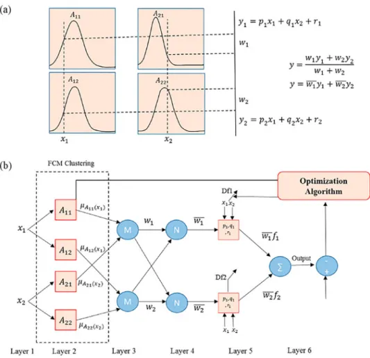
The ANFIS model is known as the acronym of the adap-tive neuro fuzzy inference system. ANFIS is an adapadap-tive fuzzy based model that is developed by using the com-putation ability of the ANNs (Jang & Gulley,1995). The ANFIS is a Sugeno type of fuzzy model that has a pro-moting system configuration using two different clus-tering methods: grid partition and subtractive clusclus-tering (Sanikhani, Kisi, Kiafar, & Ghavidel,2015). Figure2 dis-plays a Sugeno fuzzy system that has two input param-eters, one output parameter as the result, and two rules. The corresponding ANFIS structure of this system is also presented in Figure2(Rafiei-Sardooi et al.,2018; Seifi & Riahi,2018). Its rules are:
Rule 1: If x is A1and y is B1Then f=p1x+q1y+r1
Rule 2: If x is A2and y is B2Then f=p2x+q2y+r2
The output of node i in j layer of ANFIS model is Oij
(Jang & Gulley,1995). Moreover, its layers from input to output are:
First layer, input variables: in this layer any input is
imagined to fuzzy set by corresponding to the member-ship degree of bell shape membermember-ship function (Zadeh,
1965):
O1i = 1
1+[(x−ci)/ai]2bi
(6) X is the input variable i, and ci, bi and ai are the
con-stants of fuzzy membership function and usually called if (condition) parameters.
Figure 2.The structure of the Sugeno fuzzy system, its membership function, and equivalent ANFIS structure.
Second layer, rule grids:the grade of activation of
incor-porated rules is evaluated:
O2i =wi=μAi(x)×μBi(y),i=1, 2
in which the mAi(x) is the membership degree of input
variable x in Ai, and mBi(x) is for y in Birespectively.
Third layer, intermediate grids:this layer calculates
rel-ative activation degree: O3i =wni = wi
w1+w2, i=1, 2 (7)
and the winis the normalization of each rule i
member-ship degree.
Fourth layer, consequent grids:here the output of layers
is determined:
O4i =wnifi=wni.(pi+qi+ri), i=1, 2
The ri, qi, and piare the regulatory constants that should
be calculated in the optimization procedure and known as the result constants.
Fifth layer, final result layer: the overall result of the
system is evaluated O5i =wnifi = wifi wi (8)
in this study by comparing different structures. Finally, the gbellmf: generalized bell-shaped membership func-tion is used with a three membership funcfunc-tion for each rule and the hybrid learning algorithm is used for train-ing the ANFIS model.
2.4. Multi-linear regression
Another model that is used in the present paper is lin-ear regression. In the case that the output parameter Y is related to the m input parameters X1, X2,. . .,Xm
and a linear relation is supposed to show the depen-dences of Y to Xi, the multiple linear equation of Y is Y=a+b1×1+b2×2+ . . .+bmxm.
y in this model displays the estimated value of the parameter Y in regard to the input parameters of X1 =x1, X2=x2,. . .,Xm =xm. The multi-linear
minimizing the sum of the eyidifferences of measured
values from the model determined by the regression model (Kisi & Cobaner,2009):
N i=1 e2yi= N i=1 (yi−a−b1x1i−b2x2i−bmxmi)2 (15)
In the present study, the constants a, b1, b2,. . . ,bm
are derived by least squares procedure (Kisi & Cobaner,
2009). The multi-linear regression model of scour on an alluvial bed downstream of water level control structures is: x z =a0+a1 b z+a2 h H +a3 b B +a4 Q/bz gdm(ρs−ρ ρ) +a5 d90 dm (9) 2.5. Multi-non-linear regression
Because of the complexity of the scour process the linear regression models are used. The multivariable non-linear least square regression (MNLR) model is used for the estimation of scour dimensions. If the output parameter f is to be a function of input parameters xi
(i= 1,. . . n):
f =f(x1,x2,. . .,xn) (10)
by using the polynomials, the functional form of this equation is (Ramamurthy, Qu, & Vo,2006):
f =g1(x1).g2(x2) . . .gn(xn)= n
i=1
gi(xi) (11)
in whichgi(xi)=several degree polynomial equation.
If fkis to be the observed value related to xik, the sum
of the square errors minimization by least square method is used to derive nonlinear regression coefficients aij:
δ2= s
k=1
(f −fk)2 (12)
In this study after several preliminary trials the following Multi-Non-Linear Regression equation was selected for
scour modeling: x z =a( b z) b(h H) c(b B) d( Q bz gdm(ρsρ−ρ) )e(d90 dm) f (13)
2.6. The data set and empirical equations
Estimation of scour hole dimensions on an alluvial bed with hydraulic water level structures using the equations of Table1, MLR, MNLR, MLP, RBF, and ANFIS mod-els needs hydraulic and geometry excremental data. A data bank of published literature was prepared and mod-els developed. The data is gathered such that it includes all necessary variables in previous studies. Table2presents the features of implemented data and variables. In all of the collected data the b and l were constant (900) and eliminated from the effective variables. A reliable data set involving 226 documented tests of scour geometry downstream of water adjusting and grade control struc-ture is compiled from literastruc-ture. The data set are used from published literature such as (D’Agostino & Ferro,
2004). Seventy-five percent of the database is used for the training stage of models; the remaining 25% is used for the testing of models, which in all of the models, training (calibration), and testing (prediction) data sets were similar (except for RBF). Training and testing sub-sets are divided randomly and the final best structure of ANN and ANFIS models were found through a trial and error process. Subsequently, different models with dif-ferent layers and parameters were developed and finally the optimum structure of ANN and ANFIS models was determined and the results of optimum model compared with other models. All the data was dimensionless and based on dimensionless parameters of Equation (2). Fur-thermore, in ANN models based on the maximum and minimum values, the dimensionless variables normal-ized between (0.2 - 0.8). The dataset of the present study is presented in‘’ Appendix 1.
The empirical equations are the equations that have been developed by different authors in previous liter-ature. Those used in the present study are presented in Table1. In Table 1the available empirical equations for the hole scouring dimensions predictions with their
Table 2.The statistical indices of the collected data set.
Author (year) Number of data Range of hd (m) Range of XD (m) Range of XS (m) Range of S (m) Veronese (1937) 36 ***** ***** ***** .05–.22 Mossa (1998) 19 ***** ***** 0.17–.67 .035–.145 D’Agostino (1994) 114 0.045–0.255 0.43–1.75 .215–.705 .045–.85 D’Agostino and Ferro (2004) 113 ***** ***** ***** .15–.65 Falciai and Giacomin (1978) 29 ***** ***** ***** .4–3.5 Lenzi, Marion, Comiti, and Gaudio (2000) 13 ***** ***** ***** .016–.053 Scimemi (1939) 3 ***** ***** ***** 5–40
Table 3.Empirical equation results in the estimation of scour hole dimensions.
Statistical parameter
NSE TS100% AARE (%) MAE RMSE R2 Scour parameter Author (year)
−14.95 1686.6 276.5 0.945 2.01 0.8 S Yen(1987)
−14.56 982.45 91.63 0.57 1.793 0.5145 S/Z D’Agostino and Ferro (2004)
0.47 434.6 33.20 0.144 0.326 0.688 S/Z D’Agostino and Ferro (2004)
0.69 56.63 17.93 0.329 0.724 0.734 XS/Z D’Agostino and Ferro (2004)
0.75 171.5 32.8 0.054 0.067 0.79 hd/Z D’Agostino and Ferro (2004)
−0.52 63.37 47.87 0.95 1.087 0.865 XD/Z D’Agostino (1994)
−12.59 44.99 12.82 0.192 0.239 0.9113 XD/Z D’Agostino and Ferro (2004) corresponding references are provided. As these
empir-ical equations are not developed in the present study and because of the limit of the size of the paper, they are not described more here. However, readers can find more details on the mentioned references. Instead, in this study, new equations are developed by using MLR and MNLR which are fully described in the previous sections.
2.7. Statistical parameters
The results of the implemented six methods are eval-uated by several statistical indices such as: correlation coefficient (R2); root mean square error (RMSE); and mean absolute error (MAE). These indices illustrate the average performance of model prediction errors. They are overall information and do not provide details about the distribution of prediction error results. In order to assess the error distribution of modes, two further sta-tistical indices that can accurately evaluate the distri-bution percent of model results are established: average absolute relative error (AARE) and threshold statistics index (TS). These not only illustrate the performance of a model in the estimation of scour dimensions by a single value, but also display the distribution of errors over all of the predictions. The TSxvalue for x% of
esti-mations illustrates the error distribution of estimated values of different models and is calculated for different AARE values. The value of TS for x% of estimation is calculated by
TSx= Yx
n .100 (14)
in which Yx is the number of estimations (from total
number of n) for each AARE value which is less than x%. Mathematical equations of RMSE, R2, NSE, MAE, and AARE statistical parameters are (Sanikhani et al.,
2018): RMSE= n i=1(Oi−Pi)2 n 0.5 (15) R2= ⎡ ⎢ ⎣ n i=1(Oi−O)(Pi−P) n i=1(Oi−O) n i=1(Pi−P) ⎤ ⎥ ⎦ 2 , NSE=1− n i=1(Oi−Pi)2 n i=1(Oi−O)2 (16) MAE= 1 n n i=1 |P−Oi| (17) AARE%= 1 n n i=1 Oi−Pi Oi ∗100 (18)
3. Results and discussions
This section provides the evaluation of the developed methods in the prediction of scour hole geometry dimen-sions and the statistical parameters for accuracy assess-ment are provided. The final results of six methods of empirical relations, MLP, RBF, ANFIS, MLR, and MNLR are presented, analyzed, compared and discussed.
Table 4.Results of the MLR model in the prediction of scour hole dimensions.
Statistical parameter
NSE TS100% AARE (%) MAE RMSE R2 Scour parameter Stage
0.66 530.82 75.19 0.185 0.289 0.659 S/Z Calibration 0.76 4.434 13.932 0.261 0.635 0.761 XS/Z Calibration 0.96 42.95 7.98 0.13 0.174 0.961 XD/Z Calibration 0.94 81.54 12.74 0.0242 0.0334 0.944 hd/Z Calibration 0.43 287.01 65.84 0.141 0.192 0.462 S/Z Testing 0.61 119.71 18.54 0.38 0.803 0.68 XS/Z Testing 0.87 64.25 9.74 0.142 0.182 0.88 XD/Z Testing 0.87 136.91 22.166 0.0288 0.0452 0.873 hd/Z Testing
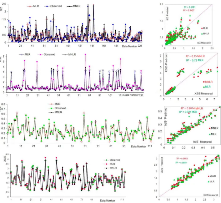
Figure 3.Comparison of estimated and observed values of score hole geometry by MLR and MNLR.
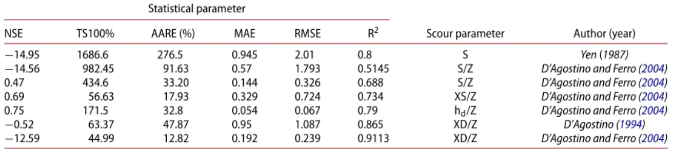
3.1. Results of empirical equations
One of the usual approaches for the estimation of grade control scour is the application of the published empir-ical equations. There are several empirempir-ical equations presented to calculate the depth and height of scour depth/deposits. In this paper, to assess the accuracy of the MLR, RBF, and ANFIS with observed values, com-parisons are also done with some of the best-known previously published equations (Table1).
The results of empirical equations in Table1for the estimation of score hole geometry are determined using the entire data set. Table3presents the statistical indices of the empirical equations of Table 1. As is clear from results in Table 3, none of these empirical equations provides acceptable estimations for scour geometry and
have substantial errors in contrast with the observa-tions. The superlative empirical equation for XD/Z is the D’Agostino and Ferro (2004) equation with R2 =0.9113, RMSE=0.239, MAE=0.192, AARE=44.9%, and TS100% =44.99. This shows that for 44.99% of estimated
values, the prediction error of model outputs are greater than 100%. That is very high and indicates the poor per-formance of available empirical equations. It is seen that while the location of the maximum deposits (XD/Z) is estimated with an acceptable accuracy, the S/Z, hd/Z, and XS/Z are estimated with less accuracy. The perfor-mance of empirical equations for other parameters of a scour hole is very poor and could not be used as accurate design methods; new methods are required. The values of these statistical indices in four scour parameters show the weak prediction of previous empirical equations for
Table 5.Results of the MNLR model in the prediction of scour hole dimensions.
Statistical parameter
NSE TS100% AARE (%) MAE RMSE R2 Scour parameter Stage
0.66 435.949 45.02 0.161 0.288 0.665 S/Z Calibration 0.77 88.74 18.392 0.303 0.622 0.771 XS/Z Calibration 0.87 28.7 6.46 0.105 0.146 0.972 XD/Z Calibration 0.93 111.34 17.52 0.029 0.038 0.93 hd/Z Calibration 0.53 259.82 38.01 0.1085 0.175 0.576 S/Z Testing 0.69 84.05 20.993 0.394 0.713 0.7135 XS/Z Testing 0.97 28.163 8.116 0.131 0.181 0.88 XD/Z Testing 0.81 150.73 26.52 0.035 0.053 0.84 hd/Z Testing
scour depth around the grade control structures. It is noticeable that the empirical equations of D’Agostino and Ferro (2004) were established by using the dataset which is used in present study, and that authors do not recalibrate these equations.
3.2. Results of the MLR model
Based on the non-dimensional parameters of Equation (2), four multi-linear regression equations are developed and their coefficients derived, which are:
S z = −0.482+0.021 b z +0.14 h h0+z−h+ 0.631B b +0.071 Q/bz gdm(ρs−ρ ρ ) +0.112d90 dm (19) XS z = −0.942+0.661 b z+0.037 h h0+z−h+2.728 B b +0.836 Q/bz gdm(ρs−ρ ρ ) −0.361d90 dm (20) hd z =0.073+0.447 b z −0.013 h h0+z−h +0.444 Q/bz gdm(ρsρ−ρ) +0.021d90 dm −0.531 B b (21) XD z =1.746+1.95 b z+0.0524 h h0+z−h +1.88 Q/bz gdm(ρsρ−ρ) −0.534d90 dm −1.99 B b (22)
The results of MLR equations in the calibration and testing stages of the dataset are provided in Table 4. With regard to these results, it is clear that although the MLR models in the calibration stage have appro-priate results, in the testing stage their results are not excellent, because of the incapability of regres-sion techniques to learn and extract the physical back-ground of scour phenomenon from the numerical val-ues of the data set. In this case the best prediction of the MLR model in the testing of the data set is for XD/Z with R2 =0.88, RMSE=0.182, MAE=0.142, AARE=9.74%, and TS100% =64.25, which shows that
the MLR model in a best situation in 64.25% of the predictions has errors greater than 100%. Moreover, the performance of the empirical equations is assessed by evaluating the scatter plot and series plots of observed and estimated values in Figure3. It could be inferred from Figure3and Table4where the scour depth (S/Z) is used, that the MLR mode appears as the lowest accurate estimations (R2=0.659 and 0.462; RMSE= 0.289 and 0.192; MAE=0.185 and 0.141; AARE(%)=75.19 and 65.84; and TS100%=530.82 and 287.01 in training and testing steps respectively). In the case of the MLR model,
Table 6.Statistical results of the MLP model in the prediction of scour hole dimensions.
Statistical parameter
NSE TS100% AARE (%) MAE RMSE R2 Scour parameter Stage
0.99 79.3 9.325 0.018 0.03 0.9964 S/Z Training 0.998 29.16 5.71 0.04 0.05 0.9985 XS/Z Training 0.997 17.81 1.94 0.029 0.045 0.9974 XD/Z Training 0.995 32.75 4.92 0.01 0.01 0.9952 Hd/Z Training 0.83 216.57 23.774 0.068 0.106 0.828 S/Z Testing 0.93 46.03 12.71 0.196 0.345 0.9514 XS/Z Testing 0.96 20.91 4.66 0.07 0.095 0.9689 XD/Z Testing 0.96 67.13 14.3 0.018 0.023 0.964 hd/Z Testing
Figure 4.Comparison of the MLP model results for S/Z, XS/Z, XD/Z, and hd/Z in training and testing steps.
the most accurate estimations are derived for XD/Z as the location of the maximum deposits.
3.3. Results of MNLR model
Using the collected data set, four multiple non-linear regression equations, based on the partial least square method for each scour variable established, are as follows:
S Z =0.539( b z) 0.149( h h0+z) 0.275(b B) −0.201 ( Q bz gdm(ρs−ρρ) )0.264(d90 dm) −0.802 (23) XS Z =1.841( b z) 0.767( h h0+z) −0.152(b B) −0.319 ( Q bz gdm(ρs−ρρ) )0.41(d90 dm) −0.254 (24) hd Z =0.452( b z) 0.64( h h0+z) 0.0207(b B) −0.752 ( Q bz gdm(ρs−ρρ) )0.704(d90 dm) −0.066 (25)
Table 7.Statistical results of the RBF model in the prediction of scour hole dimensions.
Statistical parameter
NSE TS100% AARE (%) MAE RMSE R2 Scour parameter Stage
0.89 530.54 27.63 0.0899 0.162 0.895 S/Z Training −0.157 122.342 43.9 0.083 0.084 0.998 XS/Z Training 0.98 26.61 5.317 0.084 0.12 0.98 XD/Z Training −5.68 1025.41 211.45 0.313 0.32 0.788 hd/Z Training 0.73 308.03 32.039 0.084 0.131 0.7608 S/Z Testing −0.865 102.804 52.4 0.093 0.096 0.945 XS/Z Testing 0.94 38.87 8.97 0.096 0.13 0.945 XD/Z Testing −23.18 1348.8 308.82 0.46 0.54 0.3353 hd/Z Testing
XD Z =3.328( b z) 0.423( h h0+z) 0.088(b B) −0.459 ( Q bz gdm(ρs−ρρ) )0.482(d90 dm) −0.425 (26)
Table5shows the results of the MNLR equations. In same way as with the MLR model, the MNLR model at the calibration stage has relatively proper results but at the testing stage, the error values of predictions increased. Similar with the MLR model, the best results are for
Table 8.Statistical results of the ANFIS model in the prediction of scour hole dimensions.
Statistical parameter
NSE TS100% AARE (%) MAE RMSE R2 Scour parameter Stage 0.94 219.842 25.4488 0.0753 0.125 0.9364 S/Z Training 0.9 104.8256 7.9958 0.1266 0.4103 0.9003 XS/Z Training 0.998 11.5458 2.2761 0.0333 0.0436 0.9975 XD/Z Training 0.998 11.8872 2.0178 0.0035 0.0055 0.9985 hd/Z Training 0.91 128.6585 18.7303 0.0505 0.078 0.9147 S/Z Testing 0.461 107.7542 17.5089 0.4136 0.9302 0.5669 XS/Z Testing 0.95 15.3488 5.0554 0.0805 0.1102 0.9558 XD/Z Testing 0.87 101.9133 20.6725 0.0286 0.0448 0.8790 hd/Z Testing
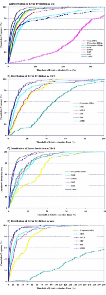
Figure 7.Error Prediction Distribution of models in (A) S/Z, (B) XS/Z, (C) XD.S, and (D) hd/z respectively.
XD/Z with R2 =0.88, RMSE=0.181, MAE=0.131, AARE=8.116, and TS100% =28.163, while for the
other scour hole parameters the MNLR model does not provide accurate results. That the MNLR model in best condition for XD/Z in 28.7% of the predictions have error values greater than 100% is also relatively high, but in comparison with the previous methods has bet-ter results. The scatbet-ter plot and series graphs of MLR and MNLR model results are compared in Figure3. In regard to the results in this figure, it is concluded that the MNLR model has somewhat better predictions than the MLR.
3.4. MLP model results
Using collected field and experimental data sets the MLP model has been trained and its optimized parameters and structures are obtained using a trial and error process. The best accuracy of tested activation and transforma-tion functransforma-tion in hidden layer was obtained by logsig, and for the output layer, it was obtained by purelin. The activation function in MLP model was logsig with five nodes in input layer, five and three nodes in two hidden layers respectively and one node in the output layer. The results of the MLP model in the training and testing and overall for the data set is presented in Table 6 and Figure 4. From this table it is concluded that the best results of the test data set come for XD/Z variable with R2 =0.97, RMSE= 0.095, MAE=0.0.07, AARE=4.66, and TS100% =20.91. Comparison of the
MLP models results in ‘’
Table6while Tables 3–5 somewhat shows the better ability of MLP models in simulating scour dimensions downstream of grade control structures. Also, the results of the MLP model in Figure 4 declare that the MLP model has accurate estimations for S/Z, XS/Z, XD/Z, and hd/Z in training and testing steps. Regarding Figure4
with Figure 3, the comparison between MLP, MNLR, and MLR shows the better function in MLP estimations. Relatively good estimations are derived from all MLP models including the five input parameters of individual data sets.
3.5. RBF model results
The results of the artificial neural network radial basis function model are provided in Table7. In this table, the best results for the training of the data sets comes for XD/Z with R2 =0.945, RMSE= 0.13, MAE=0.096, AARE=8.97, and TS100% =38.87. So the RBF model in
38.87% of the predictions have error values greater than 100% which is greater than the MLP, MNLR, and MLR models. Comparing the results in Table7with Table6
shows the superiority of the MLP model over the RB model. Also, the comparison between observed and esti-mated values of scour geometry by RBF in Figure5shows that although it has acceptable predictions for S/Z, XS/Z, and XD/Z, it has major overestimations for hd/Z. This figure shows that the developed RBF model and observed data of S/Z, XS/Z, and XS/S located near the 1:1 line with a strong data correlation in training and testing stages. These R2 values are higher than those resulting from MLR and MNLR. However, when using the RBF model for prediction of hd/Z, it demonstrates a high error, indi-cating the limitations of the RBF model when it is used to applied cases of scour deposition height estimations.
3.6. ANFIS model results
The results of the ANFIS model for three variables of scour hole geometry in several stages of model development are presented in Table 8 and Figure 6. In the training of the dataset the best predictions of the ANFIS model comes for the XD/Z with R2=0.96, RMSE=0.1102, MAE=0.0805, AARE=5.05%, and TS100% =15.3488. The ANFIS model only in 15.3488%
of predictions have errors greater than 100% and shows its ability in the prediction of scour hole length. Compar-ing the results of RBF, MLP, and empirical equations with the ANFIS model revealed that in all of four predictive parameters, the developed ANFIS model provided better results.
The worst results of ANFIS are for the location of the maximum scour depth (XS/Z) in the testing stage, while the best results of ANFIS are provided for the location of deposited sediments (XD/Z). After that there is S/Z and hd/Z in training and testing steps respectively (Figure6). Overall, based on the results of models, it can be con-cluded that the ANFIS approach is a precise model in the simulation of scour hole geometry dimensions and it can be applied for stable design of grade control structure in alluvial channels.
3.7. Comparing all models
Developing a model with a higher scale of precision in the estimation of grade control scour is of great significance in confirming the reliability and safety of water supply devices in irrigation networks and requires selecting the best estimation model. The applicability and effective-ness of the six developed models in estimating grade control scour geometry were investigated comparatively. To investigate the performance of developed models, and figure out superior models, simultaneous assessment of models are done. For this purpose the evaluation of
model results are done using error distribution of esti-mations. Comparing the results of six methods based on Tables 3–8 for four variables of S/Z, XS/Z, XD/Z, and hd/z shows that: for S/Z parameter, the maximum scour depth, the best predictions come from the ANFIS model; for XS/Z the best results is from the MLP model; for XD/Z the best prediction is from the ANFIS model; and in the hd/z variable the MLP model has the best predictions. Based on the error distribution of models in Figure7, it can be noted that the ANFIS and MLP models have esti-mated the scour geometry with approximately the same accuracy and their results are better than the others. This indicates that for all four scour parameters the intelli-gence models have superiority to the regression equations and can be used as the accurate design techniques in the design of grade control structures. Figure 7shows the error distribution of six models on all of the pre-diction variables regarding all of the data set. All devel-oped regression equations exhibit a large estimation error while the artificial intelligence models perform better due to the valuable ability to estimate scour geometry from numerical information.
The best results over training data derived for XS/Z, and hd/Z by the MLP model with R2, 0.95, and 0.96 respectively; the best predictions for S/Z and XD/Z are from ANFIS model with R2 0.91 and 0.96 respectively. The results indicated that the application of MLP and ANFIS results in the accurate prediction of scour geom-etry for the designing of stable grade control structures in alluvial irrigation channels. The MLP and ANFIS models are information-based models that use inher-ent knowledge of a phenomenon to infer the physical process behind the scour formation. The MLP model adopts its weights based on the Levenberg-Marquardt training algorithm that finds the best vector of weights of model structure; the ANFIS combines fuzzy logic as a knowledge inference engine for MLP to take advan-tage of training and uncertainties of fuzzy membership functions.
4. Conclusions
The ability to accurately estimate the whole geometry of scour holes downstream of grade control structures is important for developing irrigation regulation struc-tures. This study employed different methods and tools to improve existing empirical scour equations for grade control structures. In this paper the authors used six methods for predicting local scour on alluvial beds down-stream of grade control structures in irrigation canals. The geometry of scour holes described by four param-eters of: maximum scour depth (S); distance of S from the weir (XS); maximum height of downstream deposited
sediments (hd); and distance of hd from the weir. The
models are: empirical equations; multi layer perceptron (MLP) neural networks; radial basis functions (RBF) neural networks; adaptive neuro fuzzy inference systems (ANFIS); multiple linear regression (MLR); and multi-ple non-linear regression (MNLR). Based on the results of the study and statistical parameters and indexes it is concluded that the intelligence methods of MLP and ANFIS have more accurate predictions than RBF, MNLR, MLR, and previous equations and that the newly devel-oped models in this comparative study can be used as design methods for grade control structures. Existing studies and models, which are studied in the literature, were applicable for the estimation of only one dimension of scour geometry, while in the present study the newly developed models that are explored here were developed to estimate different dimensions of scour geometry. This led to the improvements of scour hole studies from a sin-gle parameter to a geometry space. Nevertheless, further investigations are required to improve the uncertainty of the developed methods. With all the results of mod-els considered, this paper concludes that soft computing models are superior to the classical models, but they are black box models and do not provide explicit equations for scour hole prediction. Further studies are required to derive explicit predictive equations based on ANFIS, MLP, and RBF manipulation that can be used in applica-tion design; uncertainty analysis of predicapplica-tion results also remains another improvement for future studies. Future studies also could use comparative analysis between the results from other soft computing models such as SVM, GEP, and LEM methods with the results of the developed models in the present paper. as well as with a combi-nation of ANFIS and ANN models with meta heuristic optimization algorithms as the training algorithm could be an another field for next studies.
Disclosure statement
No potential conflict of interest was reported by the authors.
Funding
This work was supported by the Ministry of Higher Education under Skim Geran Penyelidikan Fundamental (FRGS) (grant number FRGS/1/2018/ICT04/UKM/02/8).
References
ASCE Task Committee. (2000). Artificial neural networks in Hydrology. I: Preliminary concepts.Journal of Hydrologic Engineering, 5(2), 124–137.doi:10.1061/(ASCE)1084-0699 (2000)5:2(115)
Azamathulla, H. M. (2005). Neural networks to estimate scour downstream of ski-jump bucket spillway [D](Doctoral
dissertation, Ph. D. Thesis). Indian Institute of Technology, Bombay.
Azamathulla, H. M. (2012). Gene expression programming for prediction of scour depth downstream of sills.Journal of Hydrology,460-461, 156–159.doi:10.1016/j.jhydrol.2012. 06.034
Bateni, S. M., & Jeng, D. S. (2007). Estimation of pile group scour using adaptive neuro-fuzzy approach.Ocean Engineer-ing,34(8-9), 1344–1354.doi:10.1016/j.oceaneng.2006.07.003 Chang, C. K., Azamathulla, H. M., Zakaria, N. A., & Ab Ghani, A. (2012). Appraisal of soft computing tech-niques in prediction of total bed material load in tropical rivers. Journal of Earth System Science, 121(1), 125–133. doi:10.1007/s12040-012-0138-1
Chinnarasri, C., & Kositgittiwong, D. (2008, October). Labo-ratory study of maximum scour depth downstream of sills.
Proceedings of the Institution of Civil Engineers - Water Man-agement,161(5), 267–275. Thomas Telford Ltd.
Chau, K. W. (2017). Use of meta-heuristic techniques in rainfall-runoff modelling. Water, 9(3), 186. doi:10.3390/ w9030186
Choubin, B., Malekian, A., Samadi, S., Khalighi-Sigaroodi, S., & Sajedi-Hosseini, F. (2017). An ensemble forecast of semi-arid rainfall using large-scale climate predictors.Meteorological Applications,24(3), 376–386.
D’Agostino, V. (1994). Indagine sullo scavo a valle di opera trasversali mediante modellofisico a fondo mobile. L’Energia Elettrica71(2), 37–51 (in Italian).
D’Agostino, V., & Ferro, V. (2004). Scour on alluvial bed down-stream of grade-control structures. Journal of Hydraulic Engineering, 130(1), 24–37.doi:10.1061/(ASCE)0733-9429 (2004)130:1(24)
Dehghani, M., Riahi-Madvar, H., Hooshyaripor, F., Mosavi, A., Shamshirband, S., Zavadskas, E. K., & Chau, K. W. (2019). Prediction of hydropower generation using grey wolf opti-mization adaptive neuro-fuzzy inference system.Energies,
12(2), 289.
Dehghani, M., Saghafian, B., Nasiri Saleh, F., Farokhnia, A., & Noori, R. (2014). Uncertainty analysis of streamflow drought forecast using artificial neural networks and Monte-Carlo simulation.International Journal of Climatology,34, 1169–1180.doi:10.1002/joc.3754
Elnikhely, E. A. (2018). Investigation and analysis of scour downstream of a spillway.Ain Shams Engineering Journal,
9(4), 2275–2282.
Falciai, M., & Giacomin, A. (1978). Indagine Sui Gorghi Che Si Formano a Valle Delle Traverse Torrentizie.Italia Forestale Montana,23(3), 111–123. (in Italian).
Gaudio, R., Marion, A., & Bovolin, V. (2000). Morphological effects of bed sills in degrading rivers.Journal of Hydraulic Research,38(2), 89–96.doi:10.1080/00221680009498344 Goel, A., & Pal, M. (2009). Application of support
vec-tor machines in scour prediction on grade-control struc-tures.Engineering Applications of Artificial Intelligence,22(2), 216–223.doi:10.1016/j.engappai.2008.05.008
Guan, D., Melville, B., & Friedrich, H. (2016). Local scour at submerged weirs in sand-bed channels.Journal of Hydraulic Research, 54(2), 172–184. doi:10.1080/00221686.2015. 1132275
Ham, M. F., & Kostanic, I. (2001).Principles of neuro computing for Science and Engineering. New York: McGraw-Hill. Hameed, M.,Sharqi, S. S., Yaseen, Z. M., Afan, H. A., Hussain,
A., & Elshafie, A. (2017). Application of artificial intelligence (AI) techniques in water quality index prediction: A case study in tropical region, Malaysia.Neural Computing and Applications,28(1), 893–905.
Hoffmans, G. J. C. M., & Verheij, H. J. (1997).Scour Manual
(Vol. 96). Rotterdam: A.A. Balkema. CRC Press.
Hooshyaripor, F., Tahershamsi, A., & Golian, S. (2014). Application of copula method and neural networks for predicting peak outflow from breached embankments.
Journal of Hydro-Environment Research, 8(3), 292–303. doi:10.1016/j.jher.2013.11.004
Jang, J. S. R., & Gulley, N. (1995).The fuzzy logic Toolbox for Use with MATLAB. Natick, MA: The Mathworks Inc.
Juahir, H., Zain, S. M., Aris, A. Z., Yusoff, M. K., & Mokhtar, M. B. (2010). Spatial assessment of Langat river water quality using chemometrics.Journal of Environmental Monitoring,
12(1), 287–295.
Karbasi, M., & Azamathulla, H. M. (2017). Prediction of scour caused by 2D horizontal jets using soft computing techniques.Ain Shams Engineering Journal,8(4), 559–570. doi:10.1016/j.asej.2016.04.001
Khadangi, E., Madvar, H. R., & Ebadzadeh, M. M. (2009). Com-parison of ANFIS and RBF models in daily stream flow fore-casting. In2009 2nd International Conference on Computer, control and Communication(pp. 1–6). IEEE.
Khan, M., Azamathulla, H. M. D., & Tufail, M. (2012). Gene-expression programming to predict pier scour depth using laboratory data.Journal of Hydroinformatics,14, 628–645. doi:10.2166/hydro.2011.008
Kisi, O., & Cobaner, M. (2009). Modeling River stage-discharge Relationships using different neural network computing techniques.CLEAN - Soil, Air, Water,37(2), 160–169. Kumar, C., & Sreeja, P. (2012). Evaluation of selected
equa-tions for predicting scour at downstream of ski-jump spill-way using laboratory and field data.Engineering Geology,
129-130, 98–103.doi:10.1016/j.enggeo.2012.01.014 Laucelli, D., & Giustolisi, O. (2011). Scour depth modelling
by a multi-objective evolutionary paradigm.Environmental Modelling & Software,26(4), 498–509.doi:10.1016/j.envsoft. 2010.10.013
Lenzi, M. A., Marion, A., & Comiti, F. (2003). Local scouring at grade-control structures in alluvial mountain rivers.Water Resources Research,39(7),doi:10.1029/2002WR001815 Lenzi, M.A., Marion, A., Comiti, F., & Gaudio, R. (2000).
Riduzione Dello Scavo a Valle di Soglie Di Fondo Per Effetto Dell’interferenza Tra le Opere.Proc., 27th Convegno di Idraulica e Costruzioni Idrauliche, Genova,3, 271–278. (in Italian).
Lenzi, M. A., Marion, A., Comiti, F., & Gaudio, R. (2002). Local scouring in low and high gradient streams at bed sills. Journal of Hydraulic Research, 40(6), 731–739. doi:10.1080/00221680209499919
Liriano, S. L., & Day, R. A. (2001). Prediction of scour depth at culvert outlets using neural networks.Journal of Hydroinfor-matics,3(4), 231–238.doi:10.2166/hydro.2001.0021 Lu, J. Y., Hong, J. H., Chang, K. P., & Lu, T. F. (2013). Evolution
of scouring process downstream of grade-control structures under steady and unsteady flows. Hydrological Processes,
27(19), 2699–2709.doi:10.1002/hyp.9318
Marion, A., Tregnaghi, M., & Tait, S. (2006). Sediment sup-ply and local scouring at bed sills in high-gradient streams.
Water Resources Research, 42(6), doi:10.1029/2005WR0 04124
Mason, P. J., & Arumugam, K. (1985). Free Jet scour Below Dams and Flip Buckets. Journal of Hydraulic Engineer-ing,111, 220–235.doi:10.1061/(ASCE)0733-9429(1985)111: 2(220)
Melville, B. W., & Lim, S. Y. (2014). Scour caused by 2D horizontal jets. Journal of Hydraulic Engineering, 140(2), 149–155.doi:10.1061/(ASCE)HY.1943-7900.0000807 Moazenzadeh, R., Mohammadi, B., Shamshirband, S., & Chau,
K. W. (2018). Coupling a firefly algorithm with support vector regression to predict evaporation in northern Iran.
Engineering Applications of Computational Fluid Mechanics,
12(1), 584–597.
Mohammadpour, R. (2017). Prediction of local scour around complex piers using GEP and M5-Tree.Arabian Journal of Geosciences,10(18), 416.doi:10.1007/s12517-017-3203-x Mossa, M. (1998). Experimental study on the scour
down-stream of grade-control structures.Proc., 26th Convegno di Idraulica e Costruzioni Idrauliche, Catania,3, 581–594. Najafzadeh, M. (2015). Neuro-fuzzy GMDH based
parti-cle swarm optimization for prediction of scour depth at downstream of grade control structures. Engineering Sci-ence and Technology, an International Journal,18(1), 42–51. doi:10.1016/j.jestch.2014.09.002
Najafzadeh, M., Saberi-Movahed, F., & Sarkamaryan, S. (2018). NF-GMDH-Based self-organized systems to predict bridge pier scour depth under debris flow effects.Marine Geore-sources & Geotechnology, 36, 589–602. doi:10.1080/10641 19X.2017.1355944
Najah, A., El-Shafie, A., Karim, O. A., & El-Shafie, A. H. (2013). Application of artificial neural networks for water qual-ity prediction.Neural Computing and Applications, 22(1), 187–201.
Nguyen, T. H. T., Ahn, J., & Park, S. W. (2018). Numeri-cal and physiNumeri-cal investigation of the performance of Tur-bulence modeling Schemes around a scour hole down-stream of a Fixed Bed Protection. Water, 10(2), 103. doi:10.3390/w10020103
Pagliara, S. (2007). Influence of sediment gradation on scour downstream of block ramps. Journal of Hydraulic Engi-neering,133(11), 1241–1248.doi:10.1061/(ASCE)0733-9429 (2007)133:11(1241)
Pagliara, S., & Kurdistani, S. M. (2013). Scour downstream of cross-vane structures. Journal of Hydro-Environment Research,7(4), 236–242.doi:10.1016/j.jher.2013.02.002 Pandey, M., Zakwan, M., Sharma, P. K., & Ahmad, Z. (2019).
Multiple linear regression and genetic algorithm approaches to predict temporal scour depth near circular pier in non-cohesive sediment. ISH Journal of Hydraulic Engineering,
1–8.doi:10.1080/09715010.2018.1457455
Rafiei-Sardooi, E., Mohseni-Saravi, M., Barkhori, S., Azareh, A., Choubin, B., & Jafari-Shalamzar, M. (2018). Drought modeling: A comparative study between time series and neuro-fuzzy approaches. Arabian Journal of Geosciences,
11(17), 487.
Rajaei, A., Esmaeili Varaki, M., & Shafei Sabet, B. (2019). Exper-imental investigation on local scour at the downstream of grade control structures with labyrinth planform.ISH Jour-nal of Hydraulic Engineering, 1–11.doi:10.1080/09715010. 2018.1502627
Ramamurthy, A. S., Qu, J., & Vo, D. (2006). Nonlinear PLS method for side weir flows.Journal of Irrigation and Drainage Engineering, 132(5), 486–489. doi:10.1061/(ASCE)0733-9437(2006)132:5(486)
Riahi-Madvar, H., & Seifi, A. (2018). Uncertainty analysis in bed load transport prediction of gravel bed rivers by ANN and ANFIS. Arabian Journal of Geosciences, 11(21), 688. doi:10.1007/s12517-018-3968-6
Salmasi, F., Yıldırım, G., Masoodi, A., & Parsamehr, P. (2013). Predicting discharge coefficient of compound broad-crested weir by using genetic programming (GP) and artificial neu-ral network (ANN) techniques. Arabian Journal of Geo-sciences,6(7), 2709–2717.doi:10.1007/s12517-012-0540-7 Sanikhani, H., Deo, R. C., Samui, P., Kisi, O., Mert, C.,
Mirab-basi, R.,. . .Yaseen, Z. M. (2018). Survey of different data-intelligent modeling strategies for forecasting air temper-ature using geographic information as model predictors.
Computers and Electronics in Agriculture,152, 242–260. Sanikhani, H., Kisi, O., Kiafar, H., & Ghavidel, S. Z. Z. (2015).
Comparison of different data-driven approaches for model-ing lake level fluctuations: The case of Manyas and Tuz Lakes (Turkey).Water Resources Management,29(5), 1557–1574. Scimemi, E. (1939). Sulla relazione che intercede fra gli scavi
osservati nelle opere idrauliche originali e nei modelli.
Energy Elettrotecnica,16(11), 3–8.
Sarkar, A., & Dey, S. (2004). Review on local scour due to jets.
Int. J. Sediment Res,19(3), 210–238.
Scurlock, S. M., Thornton, C. I., & Abt, S. R. (2012). Equi-librium scour downstream of three-dimensional grade-control structures.Journal of Hydraulic Engineering,138(2), 167–176.doi:10.1061/(ASCE)HY.1943-7900.0000493 Seifi, A., & Riahi, H. (2018). Estimating daily reference
evapo-transpiration using hybrid gamma test-least square support vector machine, gamma test-ANN, and gamma test-ANFIS models in an arid area of Iran.Journal of Water and Climate Change.doi:10.2166/wcc.2018.003
Seifi, A., & Riahi-Madvar, H. (2019). Improving one-dimen sional pollution dispersion modeling in rivers using ANFIS and ANN-based GA optimized models.Environmental Sci-ence and Pollution Research, 26(1), 867–885. doi:10.1007/ s11356-018-3613-7
Sui, J., Faruque, M. A. A., & Balachandar, R. (2008). Influence of channel width and tailwater depth on local scour caused by square jets.Journal of Hydro-Environment Research, 2, 39–45.doi:10.1016/j.jher.2008.05.001
Taormina, R., Chau, K. W., & Sivakumar, B. (2015). Neu-ral network river forecasting through baseflow separation and binary-coded swarm optimization.Journal of Hydrology,
529, 1788–1797.
Termini, D., & Sammartano, V. (2012). Morphodynamic pro-cesses downstream of man-made structural interventions: Experimental investigation of the role of turbulent flow structures in the prediction of scour downstream of a rigid bed.Physics and Chemistry of the Earth, Parts A/B/C, 49, 18–31.doi:10.1016/j.pce.2011.12.006
Veronese, A. (1937). Erosioni di fondo a valle di un scarico.
Annali dei Lavori Pubblici,75(9), 717–726 (in Italian). Wan Mohtar, W. H. M., Afan, H., El-Shafie, A., Bong, C. H.
J., & Ab. Ghani, A. (2018). Influence of bed deposit in the prediction of incipient sediment motion in sewers using arti-ficial neural networks. Urban Water Journal, 15(4), 296– 302.
Wu, C. L., & Chau, K. W. (2011). Rainfall–runoff mod-eling using artificial neural network coupled with sin-gular spectrum analysis. Journal of Hydrology, 399(3-4), 394–409.
Yaseen, Z. M., El-Shafie, A., Afan, H. A., Hameed, M., Mohtar, W. H. M. W., & Hussain, A. (2016). RBFNN versus FFNN for daily river flow forecasting at Johor River, Malaysia.Neural Computing and Applications,27(6), 1533–1542.
Yaseen, Z. M., Sulaiman, S. O., Deo, R. C., & Chau, K. W. (2019). An enhanced extreme learning machine model for river flow forecasting: State-of-the-art, practical applications in water resource engineering area and future research direction.
Journal of Hydrology,569, 387–408.
Zadeh, L. A. (1965). Fuzzy sets.Information and Control,8(3), 338–353.
Zounemat-Kermani, M., Beheshti, A. A., Ataie-Ashtiani, B., & Sabbagh-Yazdi, S. R. (2009). Estimation of current-induced scour depth around pile groups using neural network and adaptive neuro-fuzzy inference system.Applied Soft Comput-ing,9(2), 746–755.doi:10.1016/j.asoc.2008.09.006