Asymptotically Exact TTL-Approximations of the Cache Replacement Algorithms LRU(m) and h-LRU

Asymptotically Exact TTL-Approximations of the Cache

Replacement Algorithms LRU(m) and h-LRU

Nicolas Gast, Benny Van Houdt

To cite this version:

Nicolas Gast, Benny Van Houdt. Asymptotically Exact TTL-Approximations of the Cache

Replacement Algorithms LRU(m) and h-LRU. 28th International Teletraffic Congress (ITC

28), Sep 2016, W¨

urzburg, Germany. Proceedings of the 28th ITC, 2016,

<

https://itc28.org/

>

.

<

hal-01292269

>

HAL Id: hal-01292269

https://hal.inria.fr/hal-01292269

Submitted on 22 Mar 2016

HAL

is a multi-disciplinary open access

archive for the deposit and dissemination of

sci-entific research documents, whether they are

pub-lished or not.

The documents may come from

teaching and research institutions in France or

abroad, or from public or private research centers.

L’archive ouverte pluridisciplinaire

HAL

, est

destin´

ee au d´

epˆ

ot et `

a la diffusion de documents

scientifiques de niveau recherche, publi´

es ou non,

´

emanant des ´

etablissements d’enseignement et de

recherche fran¸cais ou ´

etrangers, des laboratoires

publics ou priv´

es.

Asymptotically Exact TTL-Approximations of the

Cache Replacement Algorithms LRU(m) and h-LRU

Nicolas Gast

Benny Van Houdt

Abstract—Computer system and network performance can be significantly improved by caching frequently used information. When the cache size is limited, the cache replacement algorithm has an important impact on the effectiveness of caching. In this paper we introduce time-to-live (TTL) approximations to determine the cache hit probability of two classes of cache replacement algorithms: the recently introduced h-LRU and LRU(m). These approximations only require the requests to be generated according to a general Markovian arrival process (MAP). This includes phase-type renewal processes and the IRM model as special cases.

We provide both numerical and theoretical support for the claim that the proposed TTL approximations are asymptotically exact. In particular, we show that the transient hit probability converges to the solution of a set of ODEs (under the IRM model), where the fixed point of the set of ODEs corresponds to the TTL approximation. We further show, by using synthetic and trace-based workloads, thath-LRU and LRU(m)perform alike, while the latter requires less work when a hit/miss occurs. We also show that, as opposed to LRU,h-LRU and LRU(m) are sensitive to the correlation between consecutive inter-request times.

I. INTRODUCTION

Caches form a key component of many computer networks and systems. A large variety of cache replacement algorithms has been introduced and analyzed over the last few decades. A lot of the initial work existed in deriving explicit expressions for the cache content distribution using a Markov chain analysis [1]. This approach, however, is not always feasible: Even if explicit expressions can be obtained, they are often only applicable to analyze small caches, because of the time it takes to evaluate them. This gave rise to various approximation algorithms to compute cache hit probabilities and most notably to time-to-live (TTL) approximations.

The first TTL approximation was introduced for the least recently used (LRU) policy under the Independent reference model (IRM) by Cheet al. in [6]. The main idea behind this approximation is that an LRU cache behaves similar to a TTL cache. In a TTL cache, when an item enters the cache, it sets a deterministic timer with initial value T. When this timer expires the item is removed from the cache. If an item is requested before its timer expires, its timer is reset toT. When

T is fixed, an item with popularitypk is present in the cache at a random point in time with probability 1−e−pkT _and

PN

k=11−e

−pkT _{is the average number of items in the cache.}

The Che approximation [6] consists in approximating an LRU

cache of sizemby a TTL cache with characteristic timeT(m), whereT(m)is the unique solution of the fixed point equation

m=

N

X

k=1

(1−e−pkT_{). (1)}

The above TTL approximation for LRU can easily be generalized to renewal requests as well as to other simple variations of LRU and RANDOM under both IRM and renewal requests, as well as to certain network setups [3], [7], [12], [13]. All of these TTL approximations have been shown to be (very) accurate by means of numerical examples, but except for LRU in [8], no theoretical support was provided thus far. In this paper we introduce TTL approximations for two classes of cache replacement algorithms that are variants of LRU. The first class, called LRU(m), dates back to the 1980s [1], while the second, called h-LRU, was recently introduced in [12]. In fact, a TTL approximation for h-LRU was also introduced in [12], but this approximation relies on an additional approximation of independence between the different lists whenh >2. As we will show in the paper, this implies that the approximation error does not reduce to zero as the cache becomes large.

In this paper we make the following contributions:

• We present a TTL approximation for LRU(m) and h -LRU that is valid when the request process of an item is a Markovian arrival process (MAP). This includes any phase-type renewal process and the IRM model. In the special case of the IRM model, we derive simple closed-form expressions for the fixed point equations.

• Our TTL approximation for h-LRU can be computed

in linear time in h and appears to be asymptotically exact as the cache size grows, in contrast to the TTL approximation in [12] for h > 2. Numerical results for the TTL approximation for LRU(m) also suggest that it is asymptotically exact.

• We prove that, under the IRM model, the transient behavior of both h-LRU and LRU(m) converges to the unique solution of a system of ODEs as the cache size goes to infinity. Our TTL approximations correspond to the unique fixed point of the associated systems of ODEs. This provides additional support for the claim that our TTL approximations are asymptotically exact and is the main technical contribution of the paper.

• We validate the accuracy of the TTL approximation. We

show thath-LRU and LRU(m) perform alike in terms of the hit probability under both synthetic and trace-based workloads, while less work is required for LRU(m) when a hit/miss occurs.

• We indicate that both h-LRU and LRU(m) can exploit correlation in consecutive inter-request times of an item, while the hit probability of LRU is insensitive to this type of correlation.

The paper is structured as follows. We recall the definitions of LRU(m) and h-LRU in Section II. We show how to build and solve the TTL-approximation for LRU(m) in Section III-A, and for h-LRU in Section III-B. We demonstrate the accuracy of the TTL-approximation for any finite time period in Section IV. We compare LRU(m) and

h-LRU in Section V, by using synthetic data and real traces. We conclude in Section VI.

II. REPLACEMENTALGORITHMS

We consider two families of cache replacement algorithms:

h-LRU, introduced and calledk-LRU in [12], and LRU(m), introduced in [1], [9]. Both operate on a cache that can store up tom items and both are variants of LRU, which replaces the least-recently-used item in the cache. One way to regard LRU is to think of the cache as an ordered list of m items, where thei-th position is occupied by thei-th most-recently-used item. When a miss occurs, the item in the last position of the list is removed and the requested item is inserted at the front of the list. If a hit occurs on the item in positioni, item

imoves to the front of the list, meaning the items in position

1 toi−1 move back one position.

The h-LRU replacement algorithm: h-LRU manages a cache of sizemby making use ofh−1additional virtual lists of sizem(called list1 to listh−1) in which only meta-data is stored and one list of size mthat correspond to the actual cache (called listh). Each list is ordered, and the item in the

ith position of list`is theith most-recently-used item among the items in list`. When itemk is requested, two operations are performed:

• For each list`in which itemkappears (say in a position i), the itemkmoves to the first position of list`and the items in positions1 toi−1 move back one position.

• For each list ` in which item k does not appear but appears in list`−1, itemkis inserted in the first position of list `, all other items of list ` are moved back one position and the item that was in positionm of list ` is discarded from list`.

List 1 ofh-LRU behaves exactly as LRU, except that only the meta-data of the items is stored. Also, an item can appear in any subset of thehlists at the same time. This implies that a request can lead to as many ashlist updates. Note that there is no need for all of thehlists to have the same sizem.

The LRU(m) replacement algorithm: LRU(m) makes use of hlists of sizesm1, . . . , mh, where the first few lists may be virtual, i.e., contain meta-data only. If the first v lists are virtual we havemv+1+· · ·+mh=m(that is, only the items in listsv+ 1tohare stored in the cache). With LRU(m) each item appears in at most one of the hlists at any given time. Upon each request of an item:

• If this item is not in the cache, it moves to the first position of list 1and all other items of list1 move back one position. The item that was in position m1 of list 1

is discarded.

• If this item is in positioni of a list` < h, it is removed from list `and inserted in the first position of list `+ 1. All other items of list`+ 1move back one position and the item in the last position of list`+ 1is removed from list `+ 1 and inserted in the first position of list`. All previous items from position 1 to i−1 of list ` move back one position.

• If this item is in positioniof listh, then this item moves

to the first position of listh. All items that are in position

1 toi−1 of listhmove back one position.

When using only one list, LRU(m) coincides with LRU, and therefore with1-LRU.

III. TTL-APPROXIMATIONS

A. TTL-approximation for LRU(m)

1) IRM setting: Under the IRM model the string of re-quested items is a set of i.i.d. random variables, where itemk

is requested with probability pk. As far as the hit probability is concerned this corresponds to assuming that item k is requested according to a Poisson process with rate pk.

The TTL-approximation for LRU(m) exists in assuming that, when an item is not requested, the time it spends in list

`is deterministic and independent of the item. We denote this characteristic time by T`. Let tn be the n-th time that item

k is either requested or moves from one list to another list (where we state that an item is part of list 0 when not in the cache). Using the above assumption, we define anh+ 1states discrete-time Markov chain (Xn)n≥0, where Xn is equal to the list id of the list containing item k at timetn.

With probability e−pkT` _{the time between two requests for}

itemk exceedsT`. Hence, the transition matrix of (Xn)n is

Pk =        0 1 e−pkT1 _{0 1−e}−pkT1 . ._. . ._. . ._. e−pkTh−1 _{0 1−e}−pkTh−1 e−pkTh ₁−_e−pkTh        .

The Markov chain Xn is a discrete-time birth-death process. Hence, its steady state vector(πk,0, πk,1, . . . , πk,h)obeys

πk,`=πk,0 Q`−1 s=1(1−e −pkTs₎ Q` s=1e−pkTs =πk,0epkT` `−1 Y s=1 (epkTs_−1), (2)

for `= 1, . . . , h.

Further for`∈ {1, . . . , h}, the average time spend in `is

E[tn+1−tn|Xn=`] = Z T` t=0 e−pkt_dt=1−e −pkT` pk ,

and E[tn+1−tn|Xn = 0] = 1/pk. Combined with (2), this implies that when observing the system at a random point in time, that itemkis in list `≥1 with probability

πk,`E[tn+1−tn|Xn=`] h X j=0 πk,jE[tn+1−tn|Xn=j] = (e pkT1_{−1). . .(e}pkT` ₋₁₎ 1+ h X j=1 (epkT1_{−1). . .(e}pkTj₋₁₎

The expected number of items part of list ` is the sum of the previous expression over all items k. As for the Che approximation, setting this sum equal to m` leads to the following set of fixed point equations forT1 toTh:

m`= n X k=1 (epkT1<sub>−1). . .(e</sub>pkT`₋₁₎ 1 +Ph j=1(epkT1−1). . .(epkTj −1) . (3)

An iterative algorithm used to determine a solution of this set of fixed point equations is presented in Appendix A. In the next section we generalize this approximation to MAP arrivals. 2) MAP arrivals: We now assume that the times that item k is requested are captured by a Markovian Arrival Process (MAP). MAPs have been developed with the aim of fitting a compact Markov model to workloads with statistical correlations and non-exponential distributions [5], [14]. A MAP is characterized by two d×d matrices (D₀(k), D(₁k)), where the entry(j, j0)ofD(₁k)is the transition rate from state

j toj0 that is accompanied by an arrival and the entry (j, j0)

of D₀(k) is the transition rate from statej toj0 (withj 6=j0) without arrival. Letφ(k)_{such thatφ}(k)_(D(k)

0 +D

(k)

1 ) =0and

φ(k)_{e= 1. Note, the request rateλ}

kof itemkcan be expressed as λk = θ(k)D (k) 1 e. Setting D (k) 0 = −pk and D (k) 1 = pk

corresponds to the IRM case and letting D₁(k)=−D(₀k)ev(k)

implies that item k is requested according to a phase-type renewal process characterized by(v(k)_{, D}(k)

0 ).

Extending the previous section, we define a discrete-time Markov chain (Xn, Sn), where Xn is the list in which item

k appears and Sn is the state of the MAP process at time

tn. This Markov chain has d(h+ 1)states and its transition probability matrixPM AP_k is given by

        0 (−D(₀k))−1D(₁k) eD0(k)T1 _{0 A} k,1 . ._. . ._. . ._. eD(₀k)Th−1 _{0 A} k,h−1 eD₀(k)Th _A k,h         where Ak,`= Z T` t=0 eD(0k)T`<sub>dtD</sub>(k) 1 = (I−e D(<sub>0</sub>k)T`_)(−D(k) 0 ) −1_D(k) 1 .

Due to the block structure of PM AP

k , its steady state vector

(˜πk,0,π˜k,1, . . . ,π˜k,h)obeys ˜ πk,` = ˜πk,0 ` Y s=1 Rk,s, (4)

for `= 1, . . . , h, where the matrices Rk,s can be computed recursively as Rk,h=Ak,h−1(I−Ak,h)−1, (5) Rk,`=Ak,`−1 I−Rk,`+1eD (k) 0 T`+1 −1 , (6) for `= 1, . . . , h−1andh >1.

We also define the average time(Nk,`)j,j0that itemkspends

in state j0 in (tn, tn+1) given that Xn = (`, j), for j, j0 ∈

{1, . . . , d}. LetNk,` be the matrix with entry (j, j0)equal to

(Nk,`)j,j0, then Nk,`= Z T` t=0 eD0(k)t<sub>dt= (I</sub>−<sub>e</sub>D (k) 0 T`_)(−D(k) 0 ) −1_, for `≥1 andNk,0 = (−D (k)

0 )−1. The fixed point equations

for T1 toTh given in (3) generalize to

m`= n X k=1 ˜ πk,`Nk,`e Ph j=0π˜k,jNk,je , (7)

whereeis a column vector of ones. The hit probabilityh`in list `can subsequently be computed as

h`= 1 Pn k=1λk n X k=1 ˜ πk,`Nk,`D (k) 1 e Ph j=0˜πk,jNk,je , (8) for `= 0, . . . , h.

B. TTL-approximation for h-LRU

1) IRM setting: As in [12], our approximation forh-LRU is obtained by assuming that an item that is not requested spends a deterministic time T` in list`, independently of the identity of this item. For now we assume thatT1< T2< . . . < Th. We will show that the fixed point solutions for T1 toTh always obey these inequalities.

We start by defining a discrete-time Markov chain(Yn)n≥0

by observing the system just prior to the time epochs that item

k is requested. The state space of the Markov chain is given by {0, . . . , h}. We say thatYn = 0if item kis not in any of the lists (just prior to the nth request). Otherwise,Yn =` if item k is in list `, but is not in any of the lists `+ 1 to h. In short, the state of the Markov chain is the largest id of the lists that contain itemk.

If Yn = `, then with probability 1 −e−pkT`, item k is requested before timeT`in which case we haveYn+1=`+ 1.

Otherwise, due to our assumption thatT`≥T`−1≥. . .≥T1

all lists. Therefore the transition probability matrixP¯h,kof the

h+ 1state Markov chain (Yn)n≥0 is given by        e−pkT1 _1−e−pkT1 e−pkT2 _1−e−pkT2 .. . . .. e−pkTh _1−e−pkTh e−pkTh _1−e−pkTh        . (9) Letπ¯(h,k)_{= (¯π}(h,k) 0 , . . . ,π¯ (h,k)

h )be the stationary vector of

¯

Ph,k, then the balance equations imply:

¯ π(<sub>`</sub>h,k)=ξ`¯π (h,k) 0 ` Y s=1 (1−e−pkTs_{), (10)}

for ` = 1, . . . , h, where ξ` = 1 for ` < h and ξh =epkTh. The probabilityπ¯<sub>h</sub>(h,k)that itemkis in the cache just before a request (which by the PASTA property is also the steady-state probability for the item to be in the cache) can therefore be expressed as Qh s=1(1−e− pkTs<sub>)</sub> Qh s=1(1−e−pkTs) +e−pkTh 1 +Ph−1 `=1 Q` s=1(1−e−pkTs) . (11) Due to the nature ofh-LRU,T1can be found from analyzing LRU,T2 from 2-LRU, etc. Thus, it suffices to define a fixed point equation for Th. Under the IRM model this is simply

m = Pn

k=1¯π (h,k)

h , due to the PASTA property. These fixed point equations can be generalized without much effort to renewal arrivals as explained in Appendix B.

The following property is proven in Appendix D, where we also show thatT1< T2< . . . < Thmust hold to have a fixed point.

Proposition 1. The fixed point equation m = Pn

k=1π (h,k)

h has a unique solutionTh which is such thatTh> Th−1.

Whenh= 2Equation (11) simplifies to(1−e−pkT1₎₍₁₋

e−pkT2_)/(1−e−pkT1_+e−pkT2_{)which coincides with the hit}

probability of the so-calledrefinedmodel for 2-LRU presented in [12, Eqn (9)]. Forh >2only an approximation that relied on an additional approximation of independence between the

h lists was presented in [12, see Eqn (10)]. In Figure 1 we plotted the ratio between our approximation and the one based on (10) of [12]. The results indicate that the difference grows withh. We show in Appendix C that it typically decreases as the popular items gain in popularity.

As (11) does not rely on the additional independence ap-proximation, we expect that its approximation error is smaller and even tends to zero asmtends to infinity. This is confirmed by simulation and we list a small set of randomly chosen examples in Table I to illustrate.

2) MAP arrivals: For orderdMAP arrivals, characterized by (D₀(k), D₁(k)) for item k, we obtain a (h+ 1)d state MC by additionally keeping track of the MAP state immediately after the requests. The transition probability matrix has the same form asP¯h,k, we only need to replace the probabilities

0 200 400 600 800 1000 0.995 1 1.005 1.01 1.015 1.02 1.025 1.03 1.035 1.04 1.045 Cache Size m Refined p hit / p hit h = 1 h = 2 h = 3 h = 5 h = 10 h = 20 h = 50 n = 1000, α = 0.8

Fig. 1. Ratio of the approximation of the hit rate forh-LRU under the IRM model based on (11) and (10) of [12] as a function of the cache size for various values ofhwithn= 1000items with a Zipf-like popularity distribution with

α= 0.8.

h Simul. Eq. (10) of [12] (err) Eq. (11) (err)

n= 1000,m= 10 2 0.19826 0.20139 (+1.576%) 0.20080 (+1.277%) 3 0.21139 0.21399 (+1.230%) 0.21336 (+0.932%) 5 0.21863 0.21780 (−0.381%) 0.21994 (+0.598%) 10 0.22357 0.21912 (−1.991%) 0.22402 (+0.201%) n= 1000,m= 100 2 0.47610 0.47808 (+0.415%) 0.47641 (+0.064%) 3 0.49535 0.49695 (+0.322%) 0.49579 (+0.089%) 5 0.50777 0.50521 (−0.504%) 0.50806 (+0.056%) 10 0.51506 0.50796 (−1.380%) 0.51552 (+0.088%) n= 10000,m= 100 2 0.27322 0.27404 (+0.302%) 0.27352 (+0.109%) 3 0.28453 0.28533 (+0.281%) 0.28477 (+0.085%) 5 0.29048 0.28873 (−0.602%) 0.29065 (+0.061%) 10 0.29427 0.28991 (−1.483%) 0.29430 (+0.011%) n= 10000,m= 1000 2 0.52589 0.52746 (+0.300%) 0.52596 (+0.013%) 3 0.54340 0.54453 (+0.207%) 0.54348 (+0.015%) 5 0.55452 0.55199 (−0.455%) 0.55457 (+0.009%) 10 0.56124 0.55447 (−1.206%) 0.56130 (+0.012%) TABLE I

ACCURACY OF THE TWO APPROXIMATIONS FOR THE HIT PROBABILITY OF h-LRUUNDER THEIRMMODEL WITH AZIPF-LIKE POPULARITY DISTRIBUTION WITHα= 0.8. SIMULATION IS BASED ON10RUNS OF

103_{nREQUESTS WITH A WARM-UP PERIOD OF33%.}

of the forme−pkT` <sub>bye</sub>D0(k)T`_(−D(k) 0 )−1D (k) 1 and1−e−pkT` by(I−eD<sub>0</sub>(k)T`_)(−D(k) 0 )−1D (k)

1 . The fixed point equation for

determining Th is found as m= n X k=1 (¯π_h(h,k₋₁)+ ¯π(_hh,k))(I−eD(₀k)Th_)(−D(k) 0 )−1e 1/λk , (12) whereλk is the request rate of item kand

¯ π(<sub>`</sub>h,k)=π<sub>0</sub>(h,k) ` Y s=1 (I−eD0(k)Ts_)(−D(k) 0 )−1D (k) 1 ! Ξ`, for ` = 1, . . . , h, where Ξ` = I for ` < h and Ξh =

(I −(I−eD0(k)Th_)(−D(k) 0 )−1D

(k)

1 )−1. Finally, let ν (k) _be

the stochastic invariant vector of (−D(₀k))−1D(₁k), that is, its d entries contain the probabilities to be in state 1 to d

immediately after an arrival. Hence, π¯(₀h,k) can be computed by noting thatPh `=0π¯ (h,k) ` =ν (k)_.

IV. ASYMPTOTICEXACTNESS OF THE APPROXIMATIONS

In this section, we give evidences that the approximations presented in the previous section are asymptotically exact as the number of items tends to infinity. We first provide numerical evidence. We then show that the transient behavior of LRU(m) and h-LRU converges to a system of ODEs. By using a change of variable, these ODE can be transformed into PDEs whose fixed points are our TTL-approximations. A. Numerical procedure and validation

For LRU(m), the fixed point of Equation (7) can computed by a iterative procedure that update the values T` in a round-robin fashion. This iterative procedure is described in Appendix A and works well for up to h≈5 lists but can be slow for a large number of lists. The computation forh-LRU is much faster and scales linearly with the number of lists: by construction, the firsth−1 lists of ah-LRU cache behave like an(h−1)-LRU cache. OnceTh−1has been computed, the

right-hand side of the fixed point equation (12) is increasing inThand can therefore be easily computed with a complexity that does not depend onh.

1) Accuracy for LRU(m): We show that our TTL-approximation for LRU(m) is accurate by comparing the approximation with a simulation. We assume that the inter-request times of item k follow a hyperexponential distri-bution with rate zpk in state one and pk/z in state two, while the popularity distribution is a Zipf-like distribution with parameterα, i.e.,pk = (1/kα)/P

n i=11/i

α_{. Correlation} between consecutive inter-request times is introduced using the parameterq∈(0,1]. More precisely, let (D₀(k), D(₁k))equal

pk −z 0 0 −1/z , q z 1/z [z 1]/(z+ 1)−(1−q)D(₀k) .

The squared coefficient of variation (SCV) of the inter-request times of itemkis given by2(z2_{−z+ 1)/z−1and the lag-1}

autocorrelation of inter-request times of itemkis

ρ1= (1−q)

(1−z)2

2(1−z)2_+z.

In other words the lag-1 autocorrelation decreases linearly inq

and settingq= 1implies that the arrival process is a renewal process with hyperexponential inter-request times.

Table II compares the accuracy of the model with time consuming simulations (based on 5 runs of2·106 requests). We observe a good agreement between the TTL approximation and simulation that tends to improve with the size of the system (i.e., whenn increases from100 to1000).

2) Accuracy for h-LRU: For the IRM model the TTL approximation was already validated by simulation in Table I. Using the same numerical examples as for LRU(m) we demonstrate the accuracy of the TTL-approximation under MAP arrivals in Table III. Simulation results are based on 5

runs containing2·106_{requests each and are in good agreement}

with the TTL-approximation.

n q z method h0 h1 h2 100 1 2 model 0.26898 0.19304 0.53798 simul. 0.27021 0.19340 0.53639 10 model 0.03712 0.05889 0.90399 simul. 0.03723 0.06106 0.90171 1000 1 2 model 0.22580 0.16262 0.61158 simul. 0.22599 0.16256 0.61145 10 model 0.03112 0.04963 0.91925 simul. 0.03108 0.04969 0.91923 1000 0.1 2 model 0.21609 0.14510 0.63881 simul. 0.21603 0.14526 0.63870 10 model 0.03006 0.02044 0.94950 simul. 0.02984 0.02032 0.94985 TABLE II

ACCURACY OF PROBABILITYh`OF FINDING A REQUESTED ITEM IN LIST` FORLRU(m). IN THIS EXAMPLEα= 0.8,h= 2ANDm1=m2=n/5

(i.e.,20OR200). n q z method h= 2 h= 3 100 1 2 model 0.53619 0.54292 simul. 0.53449 0.54150 10 model 0.88249 0.83718 simul. 0.87936 0.83449 1000 1 2 model 0.61028 0.61605 simul. 0.61016 0.61587 10 model 0.90103 0.86300 simul. 0.90071 0.86262 1000 0.1 2 model 0.64744 0.65841 simul. 0.64807 0.65899 10 model 0.94935 0.94646 simul. 0.94924 0.94632 TABLE III

ACCURACY OF HIT PROBABILITY FORh-LRUWITHMAPARRIVALS. IN THIS EXAMPLEα= 0.8ANDm=n/5.

B. Asymptotic behavior and TTL-approximation

In this subsection, we construct two systems of ODEs that approximate the transient behavior of LRU(m) and h-LRU. These approximations become exact as the popularity of the most popular item decreases to zero:

Theorem 1. Let H`(t) be the sum of the popularity of

the items of list ` and h`(t) be the corresponding ODE approximation (Equation (18) for h-LRU and Equation (22) for LRU(m)). Then: for any timeT, there exists a constantC

such that E " sup t≤T /√maxkpk |H`(t)−h`(t)| # ≤Cq max k pk, where C does not depend on the probabilitiesp1. . . pn, the cache size mor the number of items n.

Our proof of this results is to use an alternative representa-tion of the state space that allows us to use techniques from stochastic approximation. We present the main ideas in this paper while the technical details are provided in Appendix E. We associate to each item k a variableτk(t)that is called therequest timeof itemkat timetand an additional variable that tracks if an item appears in a list. Our approximation is given by an ordinary differential equation (ODE) on xk,b(t) that is an approximation of the probability thatτk(t)is greater thanbwhile appearing in a list`. A more natural representation

would be to consider the time since the last request. Our ODE approximation would then be replaced a partial differential equation (PDE) by replacing the ODE in xk,`,b by a PDE in

yk,`,s, whereyk,`,s(t) =xk,`,t−s(t). However, when working directly with the PDE, the proofs are much more complex. In each case, we show that the fixed point of the PDE corresponds to the TTL-approximation of LRU(m) and h-LRU presented in Sections III-A and III-B.

To ease the presentation, we present the convergence result when the arrivals follow an IRM model, where each item k

has a probability pk of being requested at each time step. This proof can be adapted to the case of MAP arrivals but at the price of more complex notations. Indeed, for IRM, our system of ODEs is given by the variables xk,`,b(t) which are essentially an approximation of the probability for item

k to be in a list ` while having been requested between b

andt. If the arrival process of an item is modeled by a MAP withdstates, then our approximation would need to consider

xk,`,b,j(t)which would approximate the probabilities for item

kto be in statej, in list`and having being requested between

bandt. A detailed proof for the case of MAP arrivals is beyond the scope of this paper, both because of space constraints and for the sake of clarity of the exposition.

1) LRU: We first construct the ODE approximation for LRU. In this simpler case the proof of the validity of the Che-approximation could rely on a more direct argument that uses the close-form expression of the steady state distribution of LRU, as in [8]. Yet, the ideas presented in this section serve to illustrate the more complex cases ofh-LRU and LRU(m).

The request time of an itemk evolves as follows:

τk(t+ 1) =

τk(t) ifk is not requested

t+ 1 ifk is requested. (13)

At time0,τk(0) =−iif the item is in the ith position in the cache andτk(0) =−(m+ 1)if the item is not in the cache.

The cache contains m items. Let us denote1 by Θ(t) = sup{b :Pn

k=11{τk(t)≥b} ≥m} the request time of the mth

most recently requested item. When using LRU, an item that has a request time greater or equal to Θ(t) is in the cache. We denote byH(t)the sum of the popularities of items in the cache: H(t) = n X k=1 pk1{τk(t)≥Θ(t)}.

Our approximation of the probability for itemk to have a request time afterb, is given by the following ODE (forb < t):

˙

xk,b(t) =pk(1−xk,b(t)). (14) with the initial conditions that for t > 0, xk,t(t) = 0 and for t = 0, xk,b(0) = 1{τk(t)≥b}. Similarly to the stochastic

system, we define θ(t) = sup{b : Pn

k=1xk,b(t) ≥ m},

which is the time for which the sum of the approximated

1_{Throughout the paper1{}

A}is the indicator function of an eventA. It is

equal to1ifAis true and0otherwise.

probabilities of having items requested after b is equal tom. The approximation of the hit ratio for LRU is then given by

h(t) =

n

X

k=1

pkxk,θ(t)(t).

Once these variables have been defined, the key ingredient of the proof is to use the same changes of variables as in the proof of Theorem 6 of [9], which is to considerPα,b(t):

Pα,b(t) =a1−α n X k=1 (pk)α1{τk(t)≥b}, where a:= maxn

k=1pk. These variables are defined forα∈

{0,1, . . .} andb ∈ Z. The collection of variables {Pα,b}α,b describes completely the state of the system at timetand live in an set of infinite dimension.

Similarly, we define a set of functions ρα,b by ρα,b(t) =

a1−αPn

k=1(pk)αxk,b(t). The functions ρα,b are solutions of the system of ODEs d/dtρα,b(t) =fα,b(ρ), where:

fα,b(ρ) =a1−α(

X

k

(pk)α+1)−aρα+1,a(t).

The proof of the theorem, detailed in Appendix E1, relies on classical results of stochastic approximation. It uses the fact that

• the function f is Lipchitz-continuous

• f is the E[Pα,b(t+ 1)−Pα,b(t)|P(t)] =fα,b(P(t))

• The second moment of the variation ofP(t)is bounded:

EhkP(t+1)−P(t)k2_∞|Pi≤a.

Note that Equation (14) can be transformed into a PDE by considering the change of variable yk,s(t) = xk,t−s(t). The quantity yk,s(t)is an approximation of the probability for an item k to have been requested between t−s andt. The set of ordinary differential Equations (14) can then be naturally transformed in the following PDE:

∂

∂tyk,s(t) =pk(1−yk,s(t))− ∂

∂syk,s(t). (15)

The fixed point y of the PDE can be obtained by solving the equation _∂t∂y= 0. This fixed point satisfiedyk,s= 1−e−pks. For this fixed point, the quantity T = t−θ satisfies m =

Pn

k=1(1−e

−pkT_{). This equation is the same as the}

Che-approximation, given by Equation (1).

2) h-LRU: The construction for LRU can be extended to the case ofh-LRU by adding to each itemhvariablesLk,`(t)∈

{true,false}. For item k and a list `, Lk,`(t) equals true if itemkwas present in list`just after the last request2 of item

kandfalseotherwise. Similarly to the case of LRU, we define the quantity Θ`(t)to be the request time of the least recently requested item that belongs to list` at timet, that is,

Θ`(t) = sup{b: n

X

k=1

1{τk(t)≥b∧Lk,`(t)}≥m`}.

2_{Note that, after a request, an item is always inserted in list1. This implies} Lk,1(t) = true.

We then define a quantity xk,`,b(t) that is meant to be an approximation of the probability for itemkto haveτk(t)≥b andL`(t) = true.

AsL1(t)is always equal to true, the ODE approximation for xk,1,b(t)is the same as (14). Moreover, this implies that

Θ1(t)≥Θ`(t)for`≥2. For the list`= 2, the approximation is obtained by considering the evolution of L2(t). After a request,L2(t+1)istrueifτk(t)≥Θ1(t)or if (τk(t)≥Θ2(t)

andL2(t) = true). Both these events occur if (τk(t)≥Θ1(t)

and L2(t) = true) as Θ1(t) ≥ Θ2(t). This suggests that,

if the item k is requested, then, in average Lk,2(t+ 1) is

approximately xk,1,θ1(t)+xk,2,θ2(t)−xk,2,θ1(t), which leads

to the following ODE approximation forxk,2,b:

˙

xk,2,b=pk(xk,2,θ2(t)+xk,1,θ1(t)−xk,2,θ1(t)−xk,2,b), (16)

whereθ`(t) = sup{b:P n

k=1xk,`,b(t)≥m`} for`∈ {1,2}. The formulation for the third list and above is more com-plex. In Section III-B, we showed that the computation of the fixed point is simple because the quantities T` of the fixed point satisfy T1 ≤ T2· · · ≤ Th. However, for the stochastic system, we do not necessarily have3 _Θ

`(t)≥Θ`+1(t) when `≥2, which implies that the ODE approximation forh-LRU has2h−1 _terms.

Applying the reasoning of Lk,2 to compute Lk,` (` ≥ 3) involves computing the probability of (τk(t) ≥ Θ`−1(t)

and Lk,`−1(t) = true) or (τk(t) ≥ Θ`(t) and Lk,`(t) =

true). When Θ`(t) ≤ Θ`−1(t), both these events occur

if (τk(t) ≥ Θ`−1(t) and Lk,`(t) = Lk,`−1(t) = true).

This suggest that the ODE for xk,`,b(t) has to involve a term xk,{`−1,`},θ`−1(t)(t), that is an approximation for the

item k to have a request time after θ`−1(t) and such that Lk,`−1(t) = Lk,`(t) = true. Note, for ` = 2 we have

xk,{`−1,`},b(t) = xk,`,b(t) as Lk,1(t) is always true, but this

does not hold for` >2. This leads to:

˙

xk,`,b=pk(xk,`,θ`(t)+xk,`−1,θ`−1(t)

−xk,{`−1,`},max{θ`−1(t),θ`(t)}−xk,`,b), (17)

A similar reasoning can be applied to obtain an ODE for xk,{`−1,`},b(t) as a function of xk,{`−1,`},b(t),

xk,{`−2,`−1,`},b(t) and xk,{`−2,`},b(t). For example, for

`= 3 this approximation becomes

˙

xk,{2,3},b(t) =xk,2,θ2(t)+xk,3,θ1(t)−xk,{2,3},θ1(t)−xk,{2,3},b

as Lk,1(t)is always true.

The hit probability of list` used in Theorem 1 is then

h`(t) = n

X

k=1

xk,`,θ`(t)(t), (18)

where the variablesxk,`,b satisfy the above ODE.

3_{When h = 3 lists, the variables Θ}

`(t) are not always ordered. For

example, consider the case of four items{1,2,3,4} and m1 = m2 =

m3 = 3. If initially the three caches contain the three items 1,2,3. Then, after a stream of requests:4,4,3,2,1, the cache1 and3 will contain the items{1,2,3} while the cache2 will contain{1,2,4}. This implies that

t−3 = Θ2(t)<Θ3(t) = Θ1(t) =t−2.

The proof of Theorem 1 in the case of h-LRU is very similar as the one for LRU and uses the same stochastic approximation argument. Moreover, as for LRU, the ODE (16) can be transformed into a PDE by using the change of variables yk,`,s(t) = xk,`,t−s(t) and T`(t) = t−θ`(t). This PDE has a unique fixed point that corresponds to Section III-B. 3) LRU(m): The construction of the approximation and the proof for the case of LRU(m) is more involved because of discontinuities in the dynamics. We replace the request time by a quantity that we call a virtual request time that is such that the mh items that have the largest virtual request times are in listh. The nextmh−1 are in listh−1, etc. The virtual

request time of an item changes when this item is requested. If the item was in list h or h−1 prior to the request, its virtual request time becomes t+ 1. If the item was in a list

`∈ {0. . . h−2}, its virtual request time becomes the largest virtual request time of the items in list `+ 2.

The approximation of the distribution of virtual request times is then given by an ODE on the quantities xk,b(t) that are meant to be an approximation of the probability that the itemk has a virtual request time afterb:

˙

xk,b(t) =pk(xk,θ_ζb(t)(t)−1(t)−xk,b(t)), (19)

whereθ`(t)andζb(t)are defined by:

θ`(t) = sup{b: n X k=1 xk,b(t)≥mh+· · ·+m`} (20) ζb(t) = max{`:θ`(t)≤b} (21) The intuition behind Equation (19) is that the changes in

xk,b are due to the items that had a virtual request time prior tob and that now have a virtual request time b or after. This only occurs if the item had a virtual request time between

θζb(t)−1andband was requested, in which case its new virtual

request time isθζb(t)+1≥b. Otherwise, if an item had a virtual

request time prior to θζb(t)−1, then upon request it jumps to

a list ` < ζb(t)−1 and therefore its new virtual request time stays prior to b.

The hit ratio for LRU(m) used in Theorem 1 is given by

h`(t) = n

X

k=1

pk(xk,θ`+1(t)−xk,θ`(t))(t) (22)

The main difference between the proof for LRU(m) com-pared to the one of h-LRU is that the right-side of the differential equation (19) is not Lipschitz-continuous in ρ

because the list in which an item that has an virtual request timebbelongs to depends non-continuously onρ(the listζbis a discrete quantity). In Appendix E3, we explain how to prove the convergence of the stochastic approximation algorithm by using one-sided Lipschitz-continuous functions.

V. COMPARISON OFLRU(M)AND H-LRU

In this section we compare the performance of LRU(m) and

h-LRU in terms of the achieved hit probability when subject to IRM, renewal, MAP requests and trace-based simulation. A good replacement algorithm should keep popular items in the

0 50 100 150 200 0 0.1 0.2 0.3 0.4 0.5 0.6 0.7 0.8 0.9 1 Cache Size Hit Probability Zipf α_{=0.8, n = 1000,} no correlation in IRTs IRM LRU IRM 2−LRU IRM LRM(m,m) Hypo10 LRU Hypo10 2−LRU Hypo10 LRU(m,m)

Fig. 2. Hit probability as a function of the cache size for LRU, LRU(m, m) and 2-LRU under the IRM model and with hyperexponential inter-request times (withz= 10). 0 50 100 150 200 0.1 0.2 0.3 0.4 0.5 0.6 0.7 0.8 0.9 1 Cache Size Hit Probability Zipf α_{=0.8, n = 1000,} correlation in IRTs Hypo2 LRU Hypo2 2−LRU Hypo2 LRM(m,m) Hypo10 LRU Hypo10 2−LRU Hypo10 LRU(m,m)

Fig. 3. Hit probability as a function of the cache size for LRU, LRU(m, m) and2-LRU when subject to MAP arrivals (withz= 2,10andq= 1/20).

cache, but needs to be sufficiently responsive to changes in the popularity. As LRU(m) andh-LRU are clearly better suited to keep popular items in the cache than LRU, they perform better under static workloads (IRM). We demonstrate that they often also outperform LRU when the workload is dynamic. A. Synthetic (static) workloads

For the synthetic workloads we restrict ourselves to LRU,

2-LRU and LRU(m, m). The latter two algorithms both use a cache of sizemand additionally keep track of meta-data only for themitems in list1.

Figure 2 depicts the hit probability as a function of the cache size whenn= 1000, items follow a Zipf-like popularity dis-tribution with parameter0.8 under IRM and renewal requests (withz= 10, see Section IV-A1). Figure 3 shows the impact of having correlation between consecutive inter-request times (that is,q= 1/20instead ofq= 1 forz= 2,10).

One of the main observations is that LRU(m, m) performs very similar to2-LRU under IRM, renewal and MAP requests.

0 0.05 0.1 0.15 0.2 0.25 0.3 0.35 0.4 0.45 0.8 0.82 0.84 0.86 0.88 0.9 0.92 hit probability Lag−1 autocorrelation ρ₁ Zipf α=0.8, n = 1000, m = 100 LRU 2−LRU LRU(m,m) LRU(m/2,m/2)

Fig. 4. Hit probability as a function of the lag-1autocorrelationρ1for LRU, LRU(m, m), LRU(m/2, m/2) and 2-LRU when subject to MAP arrivals (withz= 10).

In fact, 2-LRU performs slightly better, unless the workload is very dynamic (z= 10andq= 1 case). Another important observation that can be drawn from comparing Figures 2 and 3 is that the hit rate of both2-LRU and LRU(m, m) significantly improves in the presence of correlation between consecutive inter-request times (that is, whenq <1), while LRU does not. Recall that LRU(m) needs to update at most one list per hit, as opposed to h-LRU. Thus, whenever both algorithms perform alike, LRU(m) may be more attractive to use.

Figure 4 shows that the hit rate of2-LRU and LRU(m, m) both increase with increasing lag-1 autocorrelation and more importantly that the hit probability of LRU is completely insensitiveto any correlation between consecutive inter-request times. Figure 4 further indicates that the hit probability also increases withρ1when splitting the cache in two lists of equal size (although the gain is less pronounced). As indicated by the following theorem, whose proof is given in Appendix F, the insensitivity of LRU is a general result.

Theorem 2. Assume that the items’ request processes are

stationary, independent of each other and that the expected number of requests per unit time is positive and finite. Then, the hit probability of LRU only depends on the inter-arrival time distribution. In particular, it does not depend on the correlation between inter-arrival time.

This theorem complements the results of Jelenkovic and Radovanovic who showed in [11], [10] that for dependent request processes, the hit probability is asymptotically, for large cache sizes, the same as in the corresponding LRU system with i.i.d. requests. Our insensitivity result is valid not just asymptotically but requires the request processes of the various items to be independent.

B. Trace-based simulation

To perform the trace-based simulations we rely on the same

4 IR cache traces as in [4, Section 4]. In this section, we only report the result for the trace collected on Monday 18th Feb

64 128 256 512 1024 2048 4096 8192 16384 32768 0.9 1 1.1 1.2 1.3 1.4 1.5 1.6 Cache Size m

hit probability / LRU hit probability

LRU LRU(m/2,m/2) LRU(m/3,m/3,m/3) LRU(m,m) LRU(m,m/2,m/2)

Fig. 5. Hit probability as a function of the cache size for LRU(m) compared to LRU using trace-based simulation.

2013. We also simulated the other traces and obtained very similar results.

The hit probability of LRU(m) with a split cache and/or virtual lists normalized by the LRU hit probability is depicted in Figure 5 as a function of the cache size m. It indicates that LRU(m) is more effective than LRU, especially when the cache is small. For small caches using a virtual list is better than splitting the cache and using both a virtual list and split cache offers only a slight additional gain. While not depicted here, we should note that using more virtual lists or splitting the cache in more parts sometimes result in a hit probability below the LRU hit probability for larger caches.

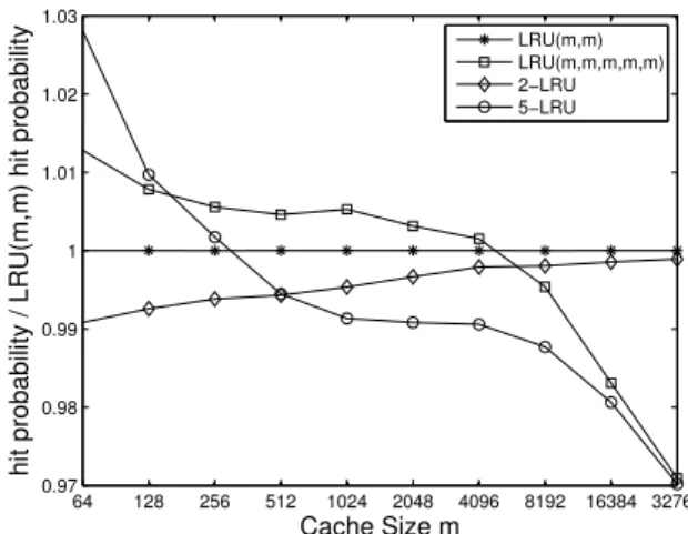
Figure 6 comparesh-LRU with LRU(m) using virtual lists, where the hit probability is now normalized by the hit prob-ability of LRU(m, m) to better highlight the differences. We observe that2-LRU differs by less than1%from LRU(m, m), while5-LRU and LRU(m, m, m, m, m) differ by less than2%. Given thath-LRU may require an update of up tohlists, while LRU(m) requires only one update in case of a hit, LRU(m) seems preferential in this particular case.

VI. CONCLUSION

In this paper, we developed algorithms to approximate the hit probability of the cache replacement policies LRU(m) andh-LRU. These algorithms rely on an equivalence between LRU-based and TTL-based cache replacement algorithms. We showed numerically that the TLL-approximations are very accurate for moderate cache sizes and appear asymptotically exact as the cache size grows. We also provide theoretical support for this claim, by establishing a bound between the transient dynamics of both policies and a set of ODEs whose fixed-point coincides with the proposed TTL-approximation.

A possible extension of our results would be to study net-works of caches in which LRU, LRU(m) orh-LRU is used in each node. Further, our TTL-approximation with MAP arrivals can be readily adapted to other policies such as FIFO(m) and RAND(m) introduced in [9]. In fact, a generalization to a

64 128 256 512 1024 2048 4096 8192 16384 32768 0.97 0.98 0.99 1 1.01 1.02 1.03 Cache Size m

hit probability / LRU(m,m) hit probability

LRU(m,m) LRU(m,m,m,m,m) 2−LRU 5−LRU

Fig. 6. Hit probability as a function of the cache size for

LRU(m, m, m, m, m) and h-LRU compared to LRU(m, m) using

trace-based simulation.

network of caches would be fairly straightforward for the class of RAND(m) policies.

REFERENCES

[1] O. I. Aven, E. G. Coffman, Jr., and Y. A. Kogan.Stochastic Analysis of Computer Storage. Kluwer Academic Publishers, Norwell, MA, USA, 1987.

[2] F. Baccelli and P. Br´emaud. Elements of queueing theory: Palm Martingale calculus and stochastic recurrences, volume 26. Springer Science & Business Media, 2013.

[3] D. S. Berger, P. Gland, S. Singla, and F. Ciucu. Exact analysis of TTL cache networks.Performance Evaluation, 79:2–23, 2014.

[4] G. Bianchi, A. Detti, A. Caponi, and N. Blefari-Melazzi. Check before storing: What is the performance price of content integrity verification in LRU caching?SIGCOMM Comput. Commun. Rev., 43(3):59–67, July 2013.

[5] G. Casale. Building accurate workload models using markovian arrival processes. InACM SIGMETRICS, SIGMETRICS ’11, pages 357–358, New York, NY, USA, 2011. ACM.

[6] H. Che, Y. Tung, and Z. Wang. Hierarchical web caching systems: modeling, design and experimental results. IEEE J.Sel. A. Commun., 20(7):1305–1314, 2002.

[7] N. C. Fofack, P. Nain, G. Neglia, and D. Towsley. Analysis of TTL-based cache networks. InValuetools 2012, pages 1–10. IEEE, 2012. [8] C. Fricker, P. Robert, and J. Roberts. A versatile and accurate

ap-proximation for LRU cache performance. InProceedings of the 24th International Teletraffic Congress, ITC ’12, pages 8:1–8, 2012. [9] N. Gast and B. Van Houdt. Transient and steady-state regime of a

family of list-based cache replacement algorithms. InProceedings of ACM SIGMETRICS. ACM, 2015.

[10] P. Jelenkovic and A. Radovanovic. Asymptotic insensitivity of least-recently-used caching to statistical dependency. InINFOCOM 2003. Twenty-Second Annual Joint Conference of the IEEE Computer and Communications. IEEE Societies, volume 1, pages 438–447. IEEE, 2003.

[11] P. R. Jelenkovi´c and A. Radovanovi´c. Least-recently-used caching with dependent requests. Theoretical computer science, 326(1):293–327, 2004.

[12] V. Martina, M. Garetto, and E. Leonardi. A unified approach to the performance analysis of caching systems. InINFOCOM 2014, pages 2040–2048, 2014.

[13] E. J. Rosensweig, J. Kurose, and D. Towsley. Approximate models for general cache networks. In INFOCOM’10, pages 1100–1108, Piscataway, NJ, USA, 2010. IEEE Press.

[14] M. Telek and G. Horv´ath. A minimal representation of markov arrival processes and a moments matching method. Perform. Eval., 64(9-12):1153–1168, Oct. 2007.

APPENDIX

A. Fixed point computations

This subsection contains some details on the computation of the fixed point for LRU(m) and h-LRU when subject to MAP arrivals. For LRU(m) the fixed point equations in case of MAP arrivals are given by (7) and an iterative algorithm to compute the fixed point is presented in Figure 1. For h-LRU we first determineT1via (12) withh= 1, then we determine

T2by considering the TTL approximation for2-LRU withT1

fixed, etc. In other words:

• forh-LRU computingT1, . . . , Th corresponds to solving

hone dimensional problems

• for LRU(m), computingT1. . . Thcorresponds to solving a singleh-dimensional one.

In practice, the computation forh-LRU is much faster.

Input:D0, D1,m1, . . . , mh,

Output: fixed point solution T1, . . . ,ˆ Tˆm

1 for`= 1 tohdo 2 Tˆ<sub>`</sub>=n; 3 end 4 Tˆh+1=∞,x= 1; 5 whilex > do 6 for`= 1 tohdo

7 Find x∈(−Tˆ`,Tˆ`+1) such that(T1, . . . , Th) equal to( ˆT1, . . . ,Tˆ`+x,Tˆ`+1−x, . . . ,Tˆh) minimizes|m`−rhs of (7)|;

8 Tˆ`= ˆT`+x;Tˆ`+1= ˆT`+1−x;

9 end

10 end

Algorithm 1: Iterative algorithm used to solve fixed point equations in(7).

B. h-LRU with renewal arrivals

The same approach as for the IRM model can be used to obtain a TTL approximation when the requests for item

k follow a renewal process, characterized by a distribution with cumulative distribution function Fk(x). Let F¯k(x) =

1−Fk(x). In this case we get ( ¯Ph,k)j,0 = ¯Fk(Tmin(h,j+1))

and( ¯Ph,k)j,min(h,j+1)=Fk(Tmin(h,j+1)). The hit probability

for itemk can therefore be expressed as

¯ π_h(h,k)= Qh s=1Fk(Ts) Qh s=1Fk(Ts) + ¯Fk(Th) 1 +Ph−1 j=1 Qj s=1Fk(Ts) ,

while forj= 1, . . . , h−1 we have

¯ π_j(h,k)= ¯ Fk(Th)Q j s=1Fk(Ts) Qh s=1Fk(Ts) + ¯Fk(Th) 1 +Ph−1 j=1 Qj s=1Fk(Ts) . 0 200 400 600 800 1000 0.975 0.98 0.985 0.99 0.995 1 1.005 1.01 1.015 1.02 1.025 Cache Size m Refined p hit / p hit n = 1000, 5−LRU α = 0.2 α _{= 0.4} α = 0.6 α = 0.8 α = 1.0 α = 1.2 α = 1.4

Fig. 7. Ratio of the approximation of the hit rate for5-LRU under the IRM model based on (11) and (10) of [12] as a function of the cache size for various values ofαwithn= 1000items with a Zipf-like popularity distribution with

α.

The fixed point equation for determining Th is found as

m= n X k=1 (¯π_h(h,k₋₁)+ ¯π(_hh,k))RTh x=0xdFk(x) R∞ x=0F¯k(x)dx = n X k=1 (¯π_h(h,k₋₁)+ ¯π_h(h,k))Th− RTh x=0Fk(x)dx R∞ x=0F¯k(x)dx , as (¯π(_hh,k₋₁)+ ¯π_h(h,k))RTh

x=0xdFk(x)is the mean time that item k spends in the cache between two requests for item k and

R∞

x=0F¯k(x)dxis simply the mean time between two requests.

C. Comparison of TTL-approximations for h-LRU

In Figure 1 we depicted the difference between our TTL-approximation forh-LRU under the IRM model based on (11) and (10) of [12], where the popularity of the items followed a Zipf-like distribution with α = 0.8. Figure 7 depicts the impact of the parameter α of the Zipf-like distribution when

h= 5. The difference between both approximations appears to grow asαdecreases. In other words, the difference decreases as the popular items gain in popularity.

D. Some proofs for h-LRU under IRM

1) Proof of Proposition 1: The fixed point equation for

h≥2 can be written asm=fh(Th), where

fh(x) = n X k=1 (1−e−pkx₎Qh−1 s=1ek,s Qh−1 s=1ek,s+e−pkx 1 +Ph−2 j=1 Qj s=1ek,s ,

with ek,s = (1−e−pkTs). The function fh(x) is clearly an increasing function inxand thereforem=f(x)has a unique

solutionTh. Further, fh(Th−1) = n X k=1 (1−e−pkTh−1₎Qh−1 s=1ek,s Qh−1 s=1ek,s+e−pkTh−1 1 +Ph−2 j=1 Qj s=1ek,s < n X k=1 Qh−1 s=1ek,s Qh−1 s=1ek,s+e−pkTh−1 1 +Ph−2 j=1 Qj s=1ek,s = n X k=1 ¯ π(_hh₋₁−1,k)=m, meaning Th> Th−1.

2) Structure of the fixed point: Using induction we prove that the fixed point solutions obeyT1< . . . < Th. We assume that T1 < . . . < Th−1 (which trivially holds for h= 2) and

show that the fixed point equation for Th does not have a solution for Th ∈ (0, Th−1). The key thing to note is that

when Th ≤ Th−1 item k is part of list h−1 whenever it

is part of list h. As such we still obtain a Markov chain by observing the system just prior to the request times, but now the last two rows of the transition probability matrix are both equal to

(e−pkTh−1_{,0, . . . ,0, e}−pkTh_−e−pkTh−1_,1−e−pkTh_).

Let(ˆπ(₀h,k), . . . ,πˆ_h(h,k))be the invariant vector of this modified Markov chain, then it is easy to see that

ˆ

π_h(h,k₋₁)+ ˆπ_h(h,k)=π_h(h₋₁−1,k),

as lumping the last two states into a single state results in the matrixP¯h−1,k. Hence the fixed point equationP

n k=1πˆ

(h,k)

h =

mcannot have a solution as n X k=1 ˆ π_h(h,k)< n X k=1 (ˆπ(_hh,k₋₁)+ ˆπ_h(h,k)) = n X k=1 ¯ π(_hh₋₁−1,k)=m. E. Proof of Theorem 1

1) LRU: Let us denotea= maxn_k=1pk. Forα∈ {0,1, . . .} andb∈Z, we definePα,b(t): Pα,b(t) =a1−α n X k=1 (pk)α1{τk(t)≥b}.

Pα,b(t)is the sum of the popularity to the powerαof all items that have a request time greater or equal tob at timet.

The collection of variables {Pα,b}α,b describe completely the state of the system at time t. They live in a set P, that is the set of infinite vectors such that there exists a vector

xk,b that is bounded by 1, non-increasing inb and such that

Pα,b=a1−αPn_k=1(pk)αxk,b.

P =n(Pα,b)α,b:∃(xk,b)non-increasing inb, bounded by1 such that for allα, b: Pα,b=a1−α

n X k=1 (pk)αxk,b o .

We equip P with the L∞ norm and denote kρk∞ =

sup_α,b|ρα,b| the norm of a vectorρ∈ P.

Similarly, we define a set of functions ρα,b by ρα,b(t) =

a1−αPn k=1(pk)

α_x

k,b(t). The functions ρα,b are solutions of the system of ODEs d/dtρα,b(t) =fα,b(ρ), where:

fα,b(ρ) =a1−α(

X

k

(pk)α+1)−aρα+1,a(t).

To prove the result, we use the following two lemmas, whose proofs are given below. The first one is a classical result from stochastic approximation that uses the fact that X(t)is noisy Euler discretization of a Lipchitz-continuous differential equation. The second lemma states that the popularity in the cache is a continuous function ofρ.

Lemma 1. Let f : P → span(P) be a

Lip-chitz continuous function with constant aL such that

sup_x∈Pkf(x)k_∞ ≤ a ≤ 1 and f(x) − x ∈ P. Let

X be a P-valued stochastic process adapted to a filtra-tion F such that E[X(t+ 1)−X(t)| Ft] = f(X(t)) and EhkX(t+ 1)−X(t)k2_∞i≤a. Then, the ODEx˙ =f(x)has a unique solutionxX(0)that starts inX(0)and for anyT >0,

E " sup t≤T /a X(t)−xX(0)(t) 2 ∞ # ≤T(2L+ 1) exp(2T L)a.

Lemma 2. Let gm : P → [0,1] be the function defined by

gm(ρ) = ρ1,θ, where θ = sup{b : ρ0,b ≥ m}. The function

gm(ρ)is Lipschitz-continuous onP with the constant 2. Let us show that f satisfies the assumption of Lemma 1. It should be clear thatf is Lipschitz-continuous with constanta. Moreover,Pα,b(t)changes if the requested item has a request time prior tob. If this item isk, thenPα,b(t+ 1) =Pα,b(t) +

a1−α_(p

k)α. This shows that E[Pα,b(t+ 1)−Pα,b(t)| Ft] = n X k=1 pka1−α(pk)α1{τk(t)<b}=fα,b(P(t))

Last, the second moment of the variation ofP(t)is bounded:

EhkP(t+1)−P(t)k2_∞|Pi=E " sup α,b |Pα,b(t+1)−Pα,b(t)| 2 |Ft # =Eh|P0,t(t+1)−P0,t(t)|2|Ft i = n X k=1 apk=a.

This implies that for eachT >0, there exists a constantC

such that Ehsup_{t≤T /a}kP(t)−ρ(t)k2_∞i ≤Ca/4. Lemma 2 concludes the proof for LRU.

Proof of Lemma 1. The solution of the ODE x˙ =f(x) that starts in X(0) satisfies x(t) = X(0)+Rt

E(t)be such that X(t) =X(0) + t−1 X s=0 f(X(s)) +E(t) =X(0) + Z t−1 0 f(X(bsc))ds+E(t). We have: kX(t)−x(t)k_∞≤ Z t s=0 kf(X(bsc))−f(x(s))k_∞+kE(t)k_∞ ≤aL Z t s=0 kX(bsc)−x(s)k_∞+kE(t)k_∞,

where we used thatf is Lipschitz-continuous of constantLa. LetX¯(t)be the the piecewise-linear interpolation ofXsuch that X¯(t) =X(t)whent∈Z+. We have:

kX(bsc)−x(s)k_∞≤X(bsc)−X¯(s) ∞+ X¯(s)−x(s) ∞ ≤a+X¯(s)−x(s) _∞,

where we used that kf(x)k_∞≤a.

This shows that for anyt≤T /a(witht∈Z+):

X¯(t)−x(t) ∞≤aL Z t s=0 X¯(s)−x(s) ∞ +a2Lt+kE(t)k_∞ ≤exp(aLt)(a2Lt+ sup

s≤t

kE(s)k_∞)

≤exp(LT)(aLT+ sup

t≤T /a

kE(t)k_∞),

using Gronwall’s inequality. By assumption, EhkE(t+ 1)−E(t)k2_∞| Ft i = var [kX(t+ 1)−X(t)| Ftk_∞] ≤EhkX(t+ 1)−X(t)k2₂| Ft i ≤a2.

AsE(t)is a martingale, this implies that E " sup t≤T /a kE(t)k2_∞ # ≤EhkE(T)k2_∞i≤aT.

Proof of Lemma 2. Let ρ, ρ0 _{∈ P. By definition of P, there}

exist x and x0 _{such that ρ}

α,b = a1−αP n k=1(pk)αxk,b and ρ0_α,b = a1−αPn k=1(pk)αx0k,b. Let θ, θ 0 _{be such that ρ} 0,θ =

ρ0_0,θ0 =m and assume without loss of generality thatθ0≤θ.

Asxk,b is non-increasing inb, this implies thatxk,θ≥xk,θ0.

Hence, we have: |ρ1,θ−ρ1,θ0|= n X k=1 pk(xk,θ−xk,θ0)≤ n X k=1 a(xk,θ−xk,θ0) =|ρ0,θ−ρ0,θ0| ≤ρ0_,θ−ρ0_0,θ0 + ρ00,θ0−ρ0,θ0 =|ρ0,θ0−ρ_0,θ0| ≤ kρ−ρ0k ∞. (23) Therefore: |gm(ρ)−gm(ρ0)|= ρ1,θ−ρ01,θ0 ≤ |ρ1,θ−ρ1,θ0|+ρ1_,θ0 −ρ0_1,θ0 ≤2kρ−ρ0k_∞,

where the last inequality comes from (23).

2) Generalization to h-LRU: The proof for h-LRU is almost identical to the proof for LRU. For simplicity, we focus on the case of 2-LRU. The proof is similar for h≥3.

We define the quantities ρα,`,b(t)andPα,`,b(t)by

ρα,`,b(t) =a1−α n X k=1 (pk)αxk,`,b(t); Pα,`,b(t) =a1−α n X k=1 (pk)α1{τk(t)≥b∧Lk,`(t)}

and Equation (16) implies that

˙

ρα,2,b=a(ρα+1,2,θ2(t)+ρα+1,1,θ1(t)

−ρα+1,2,θ1(t)−ρα+1,2,b). (24)

Lemma 2 implies that the quantity gm,`(ρ) =ρ1,`,θ, where

θ is such that ρ0,`,θ = m`, is a Lipschitz function of ρ with constant 2. It follows that the right-side of the ODE Equation (24) is Lipschitz-continuous with constant4a. As for LRU, the right side of Equation (24) is the average variation of

Pα,2,band that the second moment of the variation is bounded by a. Lemma 1 concludes the proof for 2-LRU.

As for LRU, we can transform (16) into a PDE by using the change of variables yk,`,s(t) = xk,`,t−s(t) and T`(t) =

t−θ`(t). For example, for ` = 2, the fixed point y of this PDE satisfies

0 =pk(yk,2,T2+yk,1,T1−yk,2,T1−yk,2,s)−

∂ ∂syk,2,s.

The solution of this ODE in sis given by

yk,2,s= (yk,2,T2−yk,2,T1+yk,1,T1)(1−e

−pks_{) (25)}

= yk,1,T1

1 +e−pkT2−_epkT1(1−e

−pks_{), (26)}

where we use (25) for s=T1 ands=T2 to obtain (26). In Section IV-B1, we have shown thatyk,1,T1 = 1−e

−pkT1

whereT1 is such thatPn

k=1yk,1,T1 =m. One can verify that

replacingyk,1,T1 by1−e

−pkT1 _{in Equation (26) withs=T2}

leads to Equation (11).

3) LRU(m): We now highlight the main differences with the case ofh-LRU. They are mainly due to the non-continuity of the right-side of the differential equation (19).

As before, let Pα,b(t) = a1−αP n

k=1(pk)α1{σk(t)≥b},

where a = maxn

k=1pk. We also define f : P → span(P) by fα,b(ρ) = a(ρα+1,θ_ζb−1−ρα+1,b), where θ` and ζb are two functions ofρthat are defined by

ρ0,θ` =m`+· · ·+mh andθζb≤b < θζb+1.

As for the the cases of LRU and h-LRU, one can verify that fα,b is the average variation of Pα,b(t) during one time

step and that the second moment of the average variation is bounded bya2_{. Moreover, ifxis a solution of the differential}

equation (19), then ρα,b(t) = P n

k=1xk,b(t) is a solution of the differential equationρ˙=f(ρ).

The next lemma states some key properties of the function

f. In particular,(i)quantifies what we mean by partially one-sided Lipschitz. Its proof is given below.

Lemma 3. For anyρ, ρ0∈ P and α≥1, we have:

(i) (ρ0,b−ρ00,b)(f0,b(ρ)−f0,b(ρ0))≤2akρ−ρ0k

2 ∞;

(ii) kf(ρ)k_∞≤a;

(iii) |fα,b(ρ)−fα,b(ρ0)| ≤ |f0,b(ρ)−f0,b(ρ0)|+3kρ−ρ0k_∞. Let us denote byV(t)∈ Pthe vector defined byVα,b(t) =

Pα,b(t+ 1)−Pα,b(t)−fα,b(P(t)). We haveE[V(t)| Ft] =

0 and EhkV(t)k2_∞| Ft

i

≤ a2. Moreover, the definition of

ρ(t+ 1) =ρ(t) +R₀1f(ρ(t+s))dsimplies that(P0,b(t+ 1)− ρ0,b(t+ 1))2 equals (P0,b(t)−ρ0,b(t)+V0,b(t)+f0,b(P(t))+ Z 1 0 f0,b(ρ(t+s))ds)2 = (P0,b(t)−ρ0,b(t))2+ h V0,b(t) +f0,b(P(t)) + Z 1 0 f0,b(ρ(t+s))ds i2 +2 P0,b(t)−ρ0,b(t) V0,b(t) +2P0,b(t)−ρ0,b(t) f0,b(P(t))+ Z 1 0 f0,b(ρ(t+s))ds (27) In expectation, the second term is smaller than9a2, the third is0. Forα= 0, the last term equals

2 Z 1 0 P0,b(t)−ρ0,b(t) f0,b(P(t)) +f0,b(ρ(t+s)) ds = 2 Z 1 0 P0,b(t)−ρ0,b(t+s) f0,b(P(t)) +f0,b(ρ(t+s)) ds + 2 Z 1 0 ρ0,b(t+s)−ρ0,b(t) f0,b(P(t)) +f0,b(ρ(t+s)) ds ≤4a Z 1 0 kP(t)−ρ(t+s)k2_∞ds+ 2a2, (28) where we use Lemma 3(i) to bound the first term of the equality and Lemma 3(ii) for the second.

AsPα,b(b) =ρα,b(b), Lemma 3(iii) implies that

|Pα,b(t)−ρα,b(t)| ≤ Z t s=b |f0,b(P(bsc))−f0,b(ρ(s))|ds + 3 Z t s=b kP(bsc)−ρ(s)k_∞ds+ t−1 X s=b |Vα,b(s)|. (29) Asζb(t)is a decreasing function of time that can take at most

hvalues, it can be shown that

Z t s=b |f0,b(P(bsc))−f0,b(ρ(s))|≤h Z t s=b f0,b(P(bsc))−f0,b(ρ(s)) +a Z t s=b kP(bsc)−ρ(s)k_∞ (30)

Combining Equation (27), (28), (29) and (30) shows that

EhkP(t)−ρ(t)k2_∞i≤9ah Z t

0

EhkP(bsc)−ρ(s)k2_∞ids+ 14ha2t.

By Gronwall’s inequality, this is less than exp(9aht)14ha2_t,

which, when t is less thanT /athis is less thanCafor C= 14hTexp(9T h). Lemma 2 concludes the result.

Proof of Lemma 3. The function f :P →span(P) is given by

fα,b(ρ) =a(ρα+1,θ_ζb−1−ρα+1,b), (31)

whereθ` andζb are two functions ofρthat are defined by

ρ0,θ` =m`+· · ·+mh andθζb≤b < θζb+1. (32)

We begin by the proof of (i) which states that (ρ0,b−

ρ0_0,b)(f0,b(ρ)−f0,b(ρ0))≤ 2akρ−ρ0k

2

∞. Let ρ, ρ0 ∈ P and

let ζb andζb0 be defined as in Equation (32). We have

(ρ0,b−ρ00,b)(f0,b(ρ)−f0,b(ρ0)) =a(ρ0,b−ρ00,b)(ρ0α+1,b−ρα+1,b+ρα+1,θ_ζb−1−ρ 0 α+1,θ0 ζ_b0−1 ) ≤akρ−ρ0k2_∞+a(ρ0,b−ρ00,b)(ρα+1,θ_ζb−1−ρ 0 α+1,θ0 ζ0 b−1 ).

We then distinguish three cases:

• If ζb = ζb0, then we can use Lemma 2 to show that we have ρα+1,θ_ζb−1−ρ 0 α+1,θ0 ζ0_b−1 ≤ kρ−ρ0_k ∞, which implies that (ρ0,b −ρ00,b)(ρα+1,θ_ζb−1 −ρ 0 α+1,θ0 ζ_b0−1 ) ≤ kρ−ρ0k2_∞.

• If ζb > ζb0, then Equation (32) implies that ρ0,b ≥

mζb+1 +· · · +mh > ρ 0

0,b. ζb > ζb0 also implies that

ρ0_α+1,θ0 ζ_b0−1 > ρ0_α+1,θ0 ζb−1. Hence, (ρ0,b−ρ00,b)(ρα+1,θ_ζb−1−ρ 0 α+1,θ0 ζ0_b−1 ) ≤(ρ0,b−ρ00,b)(ρα+1,θ_ζb−1−ρ 0 α+1,θ0 ζb−1)≤ kρ−ρ 0_k2 ∞,

where the last inequality comes from Lemma 2.

• The case ζb< ζb0 is symmetric.

This concludes the proof of(i). Point(ii)follows directly from Equation (31).

For point(iii), we can mimic the proof of Equation (23). By definition of P, there exists non-decreasing functions xand

x0. Assume without loss of generality that θζb ≤ θ 0 ζ0 b which implies thatxk,θ_ζb ≥xk,θ0 ζ0 b

for allk∈ {1. . . n}. Thus:

ρα,θζb−1−ρ 0 α,θ0 ζb−1 = a1−α n X k=1 (pk)α(xk,θ_ζb −x0k,θ0 ζ0 b ) ≤ a1−α n X k=1 (pk)α(xk,θ_ζb−xk,θ0 ζ_b0) +kρ−ρ0k_∞ =a1−α n X k=1 (pk)α(xk,θ_ζb−xk,θ0 ζ_b0) +kρ−ρ 0_k ∞ ≤ n X k=1 pk(xk,θ_ζb−xk,θ0 ζ0 b ) +kρ−ρ0k_∞ ≤ ρ0,θζb−1−ρ 0 0,θ0 ζb−1 + 2kρ−ρ 0_k ∞

F. Proof of the Insensitivity of LRU

For each k, the requests ofk are generated according to a stationary point processRk. Fort < s,Rk[t, s)is the number of requested of itemkduring a time interval [t, s]. Letϑk(t) be the time elapsed since the last request of item k. Without loss of generality, in the rest of the proof, we assume that the request process is simple (i.e.that with probability1, the time between two consecutive requests of an item is never0). If it is not the case, one can suppress any of the two request and obtain the same behavior of the LRU cache. Hence, the process

(Rk, ϑk)is a stationary marked point process that satisfies the Hypothesis 1.1.1 of [2].

As R is stationary, the probability that the item k is requested during a time interval [t, t+x] does not depend ont. Let F˜k(x)denote this quantity. We have:

˜

Fk(x) =P[Rk[t, t+x]≥1] =P[Rk[0, x]≥1]. We also define Fk(x) that is the probability that the time between two arrivals is smaller than x. As (Rk, ϑk) is a stationary marked point process, this quantity is well defined and can be expressed as

Fk(x) =P[Rk[t, t+x]≥1| a request occurred a timet]

=P[Rk[0, x]≥1| a request occurred a time0] Note that the definition ofFk(x)only requires the processRk to be stationary. When the process is a renewal process,Fk(x) is the cumulative distribution function of the inter-request time. By the inversion formula [2, Section 1.2.4], F˜k can be expressed as a function ofFk: ˜ Fk(x) =λk Z x 0 (1−Fk(t))dt, (33) whereλk= 1/ R∞

0 (1−Fk(t))dtis the request rate of itemk.

This quantity only depends onFk and not on the correlation between two arrivals.

To conclude the proof, we remark that the probability that an itemkis in the cache when it is requested can be expressed in terms of the functionsFkandF˜`for`6=k. Indeed, LetSn,−k

be the set of permutation of {1. . . k−1}S_{{k+ 1. . . n}(i.e.}

all integers between1andnexceptk). An item is in the cache at timet if it is among themitems that were last requested. Hence, the probability for item kto be in the cache at timet

is X σ∈Sn,−k Pϑk(t)≤ϑσ(m)(t), ϑσ(1)(t)≤ · · · ≤ϑσ(n−1)(t) .

This event conditioned on the fact that itemk is requested at timetis the probability that itemkis in the cache when it is requested. Hence, the hit rate is:

X k λk X σ∈Sn,−k P ϑk(t)≤ϑσ(m)(t), ϑσ(1)(t)≤ · · · ≤ϑσ(n−1)(t) itemkis requested att .

This quantity can clearly be expressed as a function of theFk andF˜k which by Equation (33) can be expressed solely as a function of the Fk.