www.business.unsw.edu.au
School of Economics
Australian School of Business
UNSW Sydney NSW 2052 Australia
http://www.economics.unsw.edu.au
ISSN 1323-8949
ISBN 978 0 7334 2646 9
Partial Likelihood-Based Scoring Rules for
Evaluating Density Forecasts in Tails
Cees Diks, Valentyn Panchenko
and Dick van Dijk
School of Economics Discussion Paper: 2008/10
The views expressed in this paper are those of the authors and do not necessarily reflect those of the School of Economic at UNSW.
Partial Likelihood-Based Scoring Rules for
Evaluating Density Forecasts in Tails
∗
Cees Diks
†CeNDEF, Amsterdam School of Economics University of Amsterdam
Valentyn Panchenko
‡ School of Economics University of New South WalesDick van Dijk
§ Econometric Institute Erasmus University RotterdamMay 19, 2008
Abstract
We propose new scoring rules based on partial likelihood for assessing the relative out-of-sample predictive accuracy of competing density forecasts over a specific re-gion of interest, such as the left tail in financial risk management. By construction, existing scoring rules based on weighted likelihood or censored normal likelihood favor density forecasts with more probability mass in the given region, rendering predictive accuracy tests biased towards such densities. Our novel partial likelihood-based scoring rules do not suffer from this problem, as illustrated by means of Monte Carlo simulations and an empirical application to daily S&P 500 index returns.
Keywords:density forecast evaluation; scoring rules; weighted likelihood ratio scores; partial likelihood; risk management.
JEL Classification:C12; C22; C52; C53
∗We would like to thank participants at the 16th Society for Nonlinear Dynamics and Econometrics
Conference (San Francisco, April 3-4, 2008) and the New Zealand Econometric Study Group Meeting in honor of Peter C.B. Phillips (Auckland, March 7-9, 2008) as well as seminar participants at Monash University, Queensland University of Technology, the University of Amsterdam, the University of New South Wales, and the Reserve Bank of Australia for providing useful comments and suggestions.
†Corresponding author: Center for Nonlinear Dynamics in Economics and Finance, Faculty of
Eco-nomics and Business, University of Amsterdam, Roetersstraat 11, NL-1018 WB Amsterdam, The Nether-lands. E-mail:[email protected]
‡School of Economics, Faculty of Business, University of New South Wales, Sydney, NSW 2052,
Aus-tralia. E-mail:[email protected]
§Econometric Institute, Erasmus University Rotterdam, P.O. Box 1738, NL-3000 DR Rotterdam, The
1
Introduction
The interest in density forecasts is rapidly expanding in both macroeconomics and finance. Undoubtedly this is due to the increased awareness that point forecasts are not very infor-mative unless some indication of their uncertainty is provided, see Granger and Pesaran (2000) and Garrattet al.(2003) for discussions of this issue. Density forecasts, represent-ing the future probability distribution of the random variable in question, provide the most complete measure of this uncertainty. Prominent macroeconomic applications are density forecasts of output growth and inflation obtained from a variety of sources, including sta-tistical time series models (Clements and Smith, 2000), professional forecasters (Diebold
et al., 1998), and central banks and other institutions producing so-called ‘fan charts’ for these variables (Clements, 2004; Mitchell and Hall, 2005). In finance, density forecasts play a fundamental role in risk management as they form the basis for risk measures such as Value-at-Risk and Expected Shortfall, see Dowd (2005) and McNeilet al. (2005) for general overviews and Guidolin and Timmermann (2006) for a recent empirical appli-cation. In addition, density forecasts are starting to be used in other financial decision problems, such as derivative pricing (Campbell and Diebold, 2005; Taylor and Buizza, 2006) and asset allocation (Guidolin and Timmermann, 2007). It is also becoming more common to use density forecasts to assess the adequacy of predictive regression models for asset returns, including stocks (Perez-Quiros and Timmermann, 2001), interest rates (Hong et al., 2004; Egorov et al., 2006) and exchange rates (Sarno and Valente, 2005; Rapach and Wohar, 2006).
The increasing popularity of density forecasts has naturally led to the development of statistical tools for evaluating their accuracy. The techniques that have been proposed for this purpose can be classified into two groups. First, several approaches have been put forward for testing the quality of an individual density forecast, relative to the data-generating process. Following the seminal contribution of Diebold et al. (1998), the most prominent tests in this group are based on the probability integral transform (PIT) of Rosenblatt (1952). Under the null hypothesis that the density forecast is correctly speci-fied, the PITs should be uniformly distributed, while for one-step ahead density forecasts they also should be independent and identically distributed. Hence, Dieboldet al.(1998) consider a Kolmogorov-Smirnov test for departure from uniformity of the empirical PITs and several tests for temporal dependence. Alternative test statistics based on the PITs are developed in Berkowitz (2001), Bai (2003), Bai and Ng (2005), Hong and Li (2005), Li and Tkacz (2006), and Corradi and Swanson (2006a), mainly to counter the problems caused by parameter uncertainty and the assumption of correct dynamic specification un-der the null hypothesis. We refer to Clements (2005) and Corradi and Swanson (2006c) for in-depth surveys on specification tests for univariate density forecasts. An extension of the PIT-based approach to the multivariate case is considered by Dieboldet al.(1999), see also Clements and Smith (2002) for an application. For more details of multivariate PITs and goodness-of-fit tests based on these, see Breymannet al. (2003) and Berg and Bakken (2005), among others.
The second group of evaluation tests aims to compare two or more competing density forecasts. This problem of relative predictive accuracy has been considered by Sarno and Valente (2004), Mitchell and Hall (2005), Corradi and Swanson (2005, 2006b), Amisano
and Giacomini (2007) and Bao et al. (2007). All statistics in this group compare the relative distance between the competing density forecasts and the true (but unobserved) density, but in different ways. Sarno and Valente (2004) consider the integrated squared difference as distance measure, while Corradi and Swanson (2005, 2006b) employ the mean squared error between the cumulative distribution function (CDF) of the density forecast and the true CDF. The other studies in this group develop tests of equal predictive accuracy based on a comparison of the Kullback-Leibler Information Criterion (KLIC). Amisano and Giacomini (2007) provide an interesting interpretation of the KLIC-based comparison in terms of scoring rules, which are loss functions depending on the den-sity forecast and the actually observed data. In particular, it is shown that the difference between the logarithmic scoring rule for two competing density forecasts corresponds exactly to their relative KLIC values.
In many applications of density forecasts, we are mostly interested in a particular region of the density. Financial risk management is an example in case, where the main concern is obtaining an accurate description of the left tail of the distribution. Bao et al. (2004) and Amisano and Giacomini (2007) suggest weighted likelihood ratio (LR) tests based on KLIC-type scoring rules, which may be used for evaluating and comparing density forecasts in a particular region. However, as mentioned by Corradi and Swanson (2006c) measuring the accuracy of density forecasts over a specific region cannot be done in a straightforward manner using the KLIC. The problem that occurs with KLIC-based scoring rules is that they favor density forecasts which have more probability mass in the region of interest, rendering the resulting tests biased towards such density forecasts.
In this paper we demonstrate that two density forecasts can be compared on a specific region of interest in a natural way by using scoring rules based on partial likelihood (Cox, 1975). We specifically introduce two different scoring rules based on partial likelihood. The first rule considers the value of the conditional likelihood, given that the actual obser-vation lies in the region of interest. The second rule is based on the censored likelihood, where again the region of interest is used to determine if an observation is censored or not. We argue that these partial likelihood scoring rules behave better than KLIC-type rules, in that they always favor a correctly specified density forecast over an incorrect one. This is confirmed by our Monte Carlo simulations. Moreover, we find that the scoring rule based on the censored likelihood, which uses more of the relevant information present, performs better in all cases considered.
The remainder of the paper is organized as follows. In Section 2, we briefly discuss conventional scoring rules based on the KLIC distance for evaluating density forecasts and point out the problem with the weighted versions of the resulting LR tests when these are used to focus on a particular region of the density. In Sections 3 and 4, we develop alternative scoring rules based on partial likelihood, and demonstrate that these do not suf-fer from this shortcoming. This is further illustrated by means of Monte Carlo simulation experiments in Section 5, where we assess the properties of tests of equal predictive accu-racy of density forecasts with different scoring rules. We provide an empirical application concerning density forecasts for daily S&P 500 returns in Section 6, demonstrating the practical usefulness of our approach. Finally, we conclude in Section 7.
2
Scoring rules for evaluating density forecasts
Following Amisano and Giacomini (2007) we consider a stochastic process {Zt : Ω →
Rk+1}Tt=1, defined on a complete probability space(Ω,F,P), and identifyZtwith(Yt, Xt0)
0,
whereYt : Ω → Ris the real valued random variable of interest and Xt : Ω → Rk is a
vector of predictors. The information set at timetis defined asFt =σ(Z10, . . . , Z
0
t)
0
. We consider the case where two competing forecast methods are available, each producing one-step ahead density forecasts, i.e. predictive densities ofYt+1, based onFt. The
com-peting density forecasts are denoted by the probability density functions (pdfs)ftˆ(Yt+1)
andgˆt(Yt+1), respectively. As in Amisano and Giacomini (2007), by ‘forecast method’ we
mean the set of choices that the forecaster makes at the time of the prediction, including the variables Xt, the econometric model (if any), and the estimation method. The only requirement that we impose on the forecast methods is that the density forecasts depend only on the R most recent observations Zt−R+1, . . . , Zt. Forecast methods of this type
arise easily when model-based density forecasts are made and model parameters are esti-mated based on a moving window ofR observations. This finite memory simplifies the asymptotic theory of tests of equal predictive accuracy considerably, see Giacomini and White (2006). To keep the exposition as simple as possible, in this paper we will be mainly concerned with the case of comparing ‘fixed’ predictive densities for i.i.d. processes.
Our interest lies in comparing the relative performance offˆt(Yt+1)andˆgt(Yt+1), that
is, assessing which of these densities comes closest to the true but unobserved density
pt(Yt+1). One of the approaches that has been put forward for this purpose is based on
scoring rules, which are commonly used in probability forecast evaluation, see Diebold and Lopez (1996). Lahiri and Wang (2007) provide an interesting application of several such rules to the evaluation of probability forecasts of gross domestic product (GDP) de-clines, that is, a rare event comparable to Value-at-Risk violations. In the current context, a scoring rule can be considered as a loss function depending on the density forecast and the actually observed data. The general idea is to assign a high score to a density forecast if an observation falls within a region with high probability, and a low score if it falls within a region with low probability. Given a sequence of density forecasts and corre-sponding realizations of the time series variable Yt+1, competing density forecasts may
then be compared based on their average scores. Mitchell and Hall (2005), Amisano and Giacomini (2007), and Baoet al. (2007) focus on the logarithmic scoring rule
Sl( ˆft;yt+1) = log ˆft(yt+1), (1)
whereyt+1 is the observed value of the variable of interest. Based on a sequence of P
density forecasts and realizations for observationsR + 1, . . . , T ≡ R+P, the density forecastsfˆtandˆgtcan be ranked according to their average scoresP−1
PT−1
t=Rlog ˆft(yt+1)
and P−1PT−1
t=Rlog ˆgt(yt+1). The density forecast yielding the highest score would
ob-viously be the preferred one. We may also test formally whether differences in average scores are statistically significant. Defining the score difference
dlt+1 =Sl( ˆft;yt+1)−Sl(ˆgt;yt+1)
the null hypothesis of equal scores is given byH0 : E[dlt+1] = 0. This may be tested by
means of a Diebold and Mariano (1995) type statistic
dl p ˆ σ2/P d − →N(0,1), (2)
wheredlis the sample average of the score difference, that is,dl =P−1PT−1
t=Rdlt+1, and
ˆ
σ2 is a consistent estimator of the asymptotic variance ofdlt+1. Following Giacomini and White (2006), we focus on competing forecast methods rather than on competing models. This has the advantage that the test just described is still valid in case the density forecasts depend on estimates of unknown parameters, provided that a finite (rolling) window of past observations is used for parameter estimation.
Intuitively, the logarithmic scoring rule is closely related to information theoretic mea-sures of ‘goodness-of-fit’. In fact, as discussed in Mitchell and Hall (2005) and Baoet al.
(2007), the sample average of the score differencedlin (2) may be interpreted as an esti-mate of the difference in the values of the Kullback-Leibler Information Criterion (KLIC), which for the density forecastfˆtis defined as
KLIC( ˆft) = Z pt(yt+1) log pt(yt+1) ˆ ft(yt+1) ! dyt+1 =E[logpt(Yt+1)−log ˆft(Yt+1)]. (3)
Note that by taking the difference between KLIC( ˆft)and KLIC(ˆgt)the termE[logpt(Yt+1)]
drops out, which solves the problem that the true densityptis unknown. Hence, the null
hypothesis of equal logarithmic scores for the density forecastsfˆt andgˆtactually
corre-sponds with the null hypothesis of equal KLICs. Baoet al. (2007) discuss an extension to compare multiple density forecasts, where the null hypothesis to be tested is that none of the available density forecasts is more accurate than a given benchmark, in the spirit of the reality check of White (2000).
It is useful to note that both Mitchell and Hall (2005) and Baoet al. (2007) employ the same approach for testing the null hypothesis of correct specification of an individual density forecast, that is,H0 :KLIC( ˆft) = 0. The problem that the true densityptin (3) is
unknown then is circumvented by using the result established by Berkowitz (2001) that the KLIC offˆtis equal to the KLIC of the density of the inverse normal transform of the PIT
of the density forecastfˆt. Definingzf ,tˆ +1 = Φ−1( ˆFt(yt+1))withFˆt(yt+1) = Ryt+1
−∞ fˆt(y) dy
andΦthe standard normal distribution function, it holds true that
logpt(yt+1)−log ˆft(yt+1) = logqt(zf ,tˆ +1)−logφ(zf ,tˆ +1),
whereqtis the true conditional density ofzf ,tˆ +1andφis the standard normal density. This
result states that the KLIC takes the same functional form before and after the inverse nor-mal transform of{yt+1}, which is essentially a consequence of the general invariance of
the KLIC under invertible measurable coordinate transformations. Of course, in practice the densityqt is not known either, but ifftˆ is correctly specified,{zf ,tˆ +1}should behave
as an i.i.d. standard normal sequence. As discussed in Baoet al. (2007),qtmay be
then allows testing for departures ofqtfrom the standard normal. Finally, we note that the
KLIC has also been used by Mitchell and Hall (2005) and Hall and Mitchell (2007) for combining density forecasts.
2.1
Weighted scoring rules
In empirical applications of density forecasting it frequently occurs that a particular region of the density is of most interest. For example, in risk management applications such as Value-at-Risk and Expected Shortfall estimation, an accurate description of the left tail of the distribution obviously is of crucial importance. In that case, it seems natural to focus on the performance of density forecasts in the region of interest and pay less attention to (or even ignore) the remaining part of the distribution. Within the framework of scoring rules, this may be achieved by introducing a weight functionw(yt+1)to obtain aweighted
scoring rule, see Franses and van Dijk (2003) for a similar idea in the context of testing equal predictive accuracy of point forecasts. For example, Amisano and Giacomini (2007) suggest the weighted logarithmic (WL) scoring rule
Swl( ˆft;yt+1) =w(yt+1) log ˆft(yt+1) (4)
to assess the quality of the density forecastftˆ, together with the weighted average scores
P−1PT−1
t=Rw(yt+1) log ˆft(yt+1)andP
−1PT−1
t=Rw(yt+1) log ˆgt(yt+1)for ranking two
com-peting forecasts. Using the weighted score difference
dwlt+1 =Swl( ˆft;yt+1)−Swl(ˆgt;yt+1) =w(yt+1)(log ˆft(yt+1)−log ˆgt(yt+1)), (5)
the null hypothesis of equal weighted scores,H0 :E[dwlt+1] = 0, may be tested by means of
a Diebold-Mariano type test statistic of the form (2), but using the sample averagedwl =
P−1PT−1
t=Rd wl
t+1 instead of d
l
together with an estimate of the corresponding asymptotic variance ofdwl
t+1. From the discussion above, it follows that an alternative interpretation
of the resulting statistic is to say that it tests equality of the weighted KLICs offˆtandgˆt.
The weight function w(yt+1) should be positive and bounded but may otherwise be
chosen arbitrarily to focus on a particular density region of interest. For evaluation of the left tail in risk management applications, for example, we may use the ‘threshold’ weight functionw(yt+1) = I(yt+1 ≤ r), where I(A) = 1 if the eventAoccurs and zero
otherwise, for some valuer. However, we are then confronted with the problem pointed out by Corradi and Swanson (2006c) that measuring the accuracy of density forecasts over a specific region cannot be done in a straightforward manner using the KLIC or log scoring rule. In this particular case the weighted logarithmic score may be biased towards fat-tailed densities. To understand why this occurs, consider the situation where ˆ
gt(Yt+1)> fˆt(Yt+1)for allYt+1 smaller than some given valuey∗, say. Usingw(yt+1) =
I(yt+1 ≤ r) withr < y∗ in (4) implies that the weighted score difference dwlt+1 in (5) is
never positive, and strictly negative for observations below the threshold valuer, such that E[dwl
t+1]is negative. Obviously, this can have far-reaching consequences when comparing
density forecasts with different tail behavior. In particular, there will be cases where the fat-tailed distributionˆgtis favored over the thin-tailed distribution fˆt, even if the latter is
0 0.1 0.2 0.3 0.4 0.5 density N(0,1) stand. t(5) -3 -2.5-2 -1.5-1 -0.5 0 0.5 -4 -3 -2 -1 0 1 2 3 4
log likelihood ratio
y
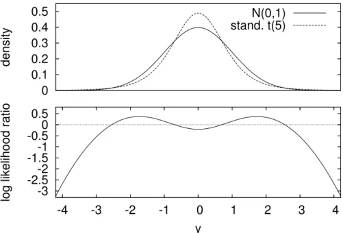
Figure 1:Probability density functions of the standard normal distributionfˆt(yt+1)and
standard-ized Student-t(5) distribution ˆgt(yt+1) (upper panel) and corresponding relative log-likelihood
scoreslog ˆft(yt+1)−log ˆgt(yt+1)(lower panel).
The following example illustrates the issue at hand. Suppose we wish to compare the accuracy of two density forecasts forYt+1, one being the standard normal distribution with
pdf ˆ ft(yt+1) = (2π)− 1 2 exp(−y2 t+1/2),
and the other being the (fat-tailed) Student-tdistribution withν degrees of freedom, stan-dardized to unit variance, with pdf
ˆ gt(yt+1) = Γ ν+12 p (ν−2)πΓ(ν2) 1 + y 2 t+1 (ν−2) −(ν+1)/2 withν >2.
Figure 1 shows these density functions for the case ν = 5, as well as the relative log-likelihood scorelog ˆft(yt+1)−log ˆgt(yt+1). The score function is negative in the left tail
(−∞, y∗), with y∗ ≈ −2.5. Now consider the average weighted log scoredwl as defined
before, based on an observed sampleyR+1, . . . , yT of P observations from an unknown
density on(−∞,∞)for whichftˆ(yt+1)andˆgt(yt+1)are candidates. Using the threshold
weight function w(yt+1) = I(yt+1 ≤ r) to concentrate on the left tail, it follows from
the lower panel of Figure 1 that if the thresholdr < y∗, the average weighted log score can never be positive and will be strictly negative whenever there are observations in the tail. Evidently the test of equal predictive accuracy will then favor the fat-tailed Student-t
densitygˆt(yt+1), even if the true density is the standard normalfˆt(yt+1).
We emphasize that the problem sketched above is not limited to the logarithmic scor-ing rule but occurs more generally. For example, Berkowitz (2001) advocates the use
of the inverse normal transform zf ,tˆ +1, as defined before, motivated by the fact that if
ˆ
ft is correctly specified, these should be an i.i.d. standard normal sequence. Taking the standard normal log-likelihood of the transformed data leads to the following scoring rule:
SN( ˆft;yt+1) = logφ(zf ,tˆ +1) = − 1 2log(2π)− 1 2z 2 ˆ f ,t+1. (6)
Although for a correctly specified density forecast the sequence{zf ,tˆ +1}is i.i.d.
nor-mal, tests for the comparative accuracy of density forecasts in a particular region based on the normal log-likelihood may be biased towards incorrect alternatives. A weighted normal scoring rule of the form
SwN( ˆft;yt+1) = w(yt+1) logφ(zf ,tˆ +1) (7)
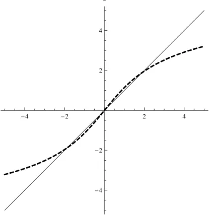
also would not guarantee that a correctly specified density forecast is preferred over an incorrectly specified density forecast. Figure 2 illustrates this point for standard normal and standardized Student-t(5)distributions, denoted asfˆtandˆgtas before. When focusing
on the left tail by using the threshold weight functionw(yt+1) =I(yt+1 ≤r), it is seen that |zf ,tˆ +1| > |zg,tˆ +1|for all values ofyless thany∗ ≈ −2. As for the weighted logarithmic
scoring rule (4), it then follows that if the threshold r < y∗ the relative score dwN t+1 = 1 2w(yt+1)(z 2 ˆ g,t+1−z 2 ˆ
f ,t+1)is strictly negative for observationsyt+1in the left tail and zero
otherwise, such that the test based on the average score differencedwN is biased against the Student-talternative.
Berkowitz (2001) proposes a different way to use the scoring rule based on the normal transform for evaluation of the accuracy of density forecasts in the left tail, based on the idea of censoring. Specifically, for a given quantile0< α <1, define the censored normal log-likelihood (CNL) score function
ScN( ˆft, yt+1) = I(Fbt(yt+1)< α) logφ(zf ,tˆ +1) +I(Fbt(yt+1)≥α) log(1−α)
=w(zf ,tˆ +1) logφ(zf ,tˆ +1) + (1−w(zf ,tˆ +1)) log(1−α), (8)
where w(zf ,tˆ +1) = I(zf ,tˆ +1 < Φ−1(α)), which is equivalent to I(Ftb(yt+1) < α). The
CNL scoring rule evaluates the shape of the density forecast for the region below theαth quantile and the frequency with which this region is visited. The latter form of (8) can also be used to focus on other regions of interest by using a weight function w(Yt+1)
equal to one in the region of interest, together withα b
f ,t = Pf ,tˆ (w(Yt+1) = 1). One can
arrange for the weight functions of competing density forecasts to coincide by allowing
α to depend on the predictive density at hand. Particularly, in the case of the threshold weight function the same thresholdrcan be used for two competing density forecasts by using two different values ofα, equal to the left exceedance probability of the valuerfor the respective density forecast.
Although it is perfectly valid to assess the quality of an individual density forecast in an absolute sense based on (8), see Berkowitz (2001), this scoring rule should be used with caution when testing the relative accuracy of competing density forecasts, as considered by Baoet al. (2004). Like the WL scoring rule, the CNL scoring rule with the threshold weight function has a tendency to favor predictive densities with more probability mass in
-4 -2 2 4 y -4 -2 2 4 z
Figure 2: Inverse normal transformations zf ,tˆ +1 = Φ−1( ˆFt(yt+1)) of the probability integral
transforms of the standard normal distribution (solid line) and the standardized Student-t(5) dis-tribution (dashed line).
the left tail. SupposeGˆt(yt+1)is fat-tailed on the left whereasFˆt(yt+1)is not. For values
ofyt+1 sufficiently far in the left tail it then holds thatFˆt(yt+1)<Gˆt(yt+1)< 12. Because
of the asymptote of Φ−1(s) at s = 0, zf ,tˆ +1 = Φ−1
ˆ
Ft(yt+1)
will be much larger in absolute value thanzˆg,t+1 = Φ−1
ˆ Gt(yt+1) , so thatφ(zf ,tˆ +1) =−12log(2π)−12zf ,t2ˆ +1 −1 2 log(2π)− 1 2z 2 ˆ
g,t+1 =φ(zˆg,t+1). That is, a much higher score is assigned to the fat-tailed
predictive densityˆgtthan tofˆt.
3
Scoring rules based on partial likelihood
The example in the previous section demonstrates that intuitively reasonable scoring rules can in fact favor the wrong density forecast when the evaluation concentrates on a partic-ular region of interest. We argue that this can be avoided by requiring that score functions correspond to the logarithm of a (partial) likelihood function associated with the outcome of some statistical experiment. To see this, note that in the standard, unweighted case the log-likelihood scorelog ˆft(yt+1)is useful for measuring the divergence between a
candi-date densityfˆtand the true densitypt, because, under the constraint
R∞
the expectation
EY[log ˆft(Yt+1)]≡E[log ˆft(Yt+1)|Yt+1 ∼pt(yt+1)]
is maximized by takingfˆt =pt. This follows from the fact that for any densityfˆtdifferent
fromptwe obtain EY " log ˆ ft(Yt+1) pt(Yt+1) !# ≤EY " ˆ ft(Yt+1) pt(Yt+1) # −1 = Z ∞ −∞ pt(y) ˆ ft(y) pt(y) dy−1≤0,
applying the inequalitylogx≤x−1tofˆt/pt.
This shows that log-likelihood scores of different forecast methods can be compared in a meaningful way, provided that the densities under consideration are properly normalized to have unit total probability. The quality of a normalized density forecastfˆtcan therefore
be quantified by the average scoreEY[log ˆft(Yt+1)]. Ifpt(y)is the true conditional density
ofYt+1, the KLIC is nonnegative and defines a divergence between the true and an
approx-imate distribution. If the true data generating process is unknown, we can still use KLIC differences to measure the relative performance of two competing densities, which renders the logarithmic score difference discussed before,dl
t+1 = log ˆft(yt+1)−log ˆgt(yt+1).
The implication from the above is that likelihood-based scoring rules may still be used to assess the (relative) accuracy of density forecasts in a particular region of the distribu-tions, as long as the scoring rules correspond to (possibly partial) likelihood functions. In the specific case of the threshold weight functionw(yt+1) = I(yt+1 ≤ r)we can break
down the observation ofYt+1 in two stages. First, it is revealed whether Yt+1 is smaller
than the threshold value r or not. We introduce the random variableVt+1 to denote the
outcome of this first stage experiment, defining it as
Vt+1 = (
1 ifYt+1 ≤r,
0 ifYt+1 > r.
(9)
In the second stage the actual valueYt+1 is observed. The second stage experiment
cor-responds to a draw from the conditional distribution of Yt+1 given the region (below or
above the threshold) in which Yt+1 lies according to the outcome of the first stage, as
indicated by Vt+1. Note that we may easily allow for a time varying threshold value rt.
However, this is not made explicit in the subsequent notation to keep the exposition as simple as possible.
Any (true or false) probability density functionftofYt+1 given Ft can be written as
the product of the probability density function ofVt+1, which is revealed in the first stage
binomial experiment, and that of the second stage experiment in which Yt+1 is drawn
from its conditional distribution givenVt+1. The likelihood function associated with the
observed valuesVt+1 = I(Yt+1 ≤ r) = v and subsequently Yt+1 = ycan thus be written
as the product of the likelihood ofVt+1, which is a Bernoulli random variable with success
probabilityF(r), and that of the realization ofYt+1givenv:
(F(r))v(1−F(r))1−v f(y) 1−F(r)I(v = 0) + f(y) F(r)I(v = 1) .
By disregarding either the information revealed byVt+1orYt+1|v (possibly depending on
the first-stage outcomeVt+1) we can construct various partial likelihood functions. This
enables us to formulate several scoring rules that may be viewed as weighted likelihood scores. As these still can be interpreted as a true (albeit partial) likelihood, they can be used for comparing the predictive accuracy of different density forecasts. In the following, we discuss two specific scoring rules as examples.
Conditional likelihood scoring rule For a given density forecast fˆt, if we decide to
ignore information from the first stage and use the information revealed in the second stage only if it turns out thatVt+1 = 1 (that is, ifYtis a tail event), we obtain the conditional
likelihood (CL) score function
Scl( ˆft;yt+1) =I(yt+1 ≤r) log( ˆft(yt+1)/Fˆt(r)). (10)
The main argument for using such a score function would be to evaluate density fore-casts based on their behavior in the left tail (values less than or equal to r). However, due to the normalization of the total tail probability we lose information of the original density forecast on how often tail observations actually occur. This is because the infor-mation regarding this frequency is revealed only by the first-stage experiment, which we have explicitly ignored here. As a result, the conditional likelihood scoring rule attaches comparable scores to density forecasts that have similar tail shapes, but completely dif-ferent tail probabilities. This tail probability is obviously relevant for risk management purposes, in particular for Value-at-Risk evaluation. Hence, the following scoring rule takes into account the tail behavior as well as the relative frequency with which the tail is visited.
Censored likelihood scoring rule Combining the information revealed by the first stage experiment with that of the second stage provided thatYt+1 is a tail event (Vt+1 = 1), we
obtain the censored likelihood (CSL) score function
Scsl( ˆft;yt+1) =I(yt+1 ≤r) log ˆft(yt+1) +I(yt+1 > r) log(1−Fˆt(r)). (11)
This scoring rule uses the information of the first stage (essentially information regarding the CDFFˆt(y)aty = r) but apart from that ignores the shape offt(y)for values above
the threshold valuer. In that sense this scoring rule is similar to that used in the Tobit model for normally distributed random variables that cannot be observed above a certain threshold value (see Tobin, 1958). To compare the censored likelihood score with the censored normal score of (8), consider the case α = ˆFt(r) in the latter. The indicator fuctions, as well as the second terms, in both scoring rules then coincide exactly, while the only difference between the scoring rules is thatlog ˆft(yt+1)occurs in the CSL rule
in place where the CNL rule has logφ(zf ,tˆ +1). It is the latter term that gave rise to the
(too) high scores in the left tail to the standardized t(5)-distribution in case the correct distribution is the standard normal.
We may test the null hypothesis of equal performance of two density forecastsftˆ(y) andˆgt(y)based on the conditional likelihood score (10) or the censored likelihood score
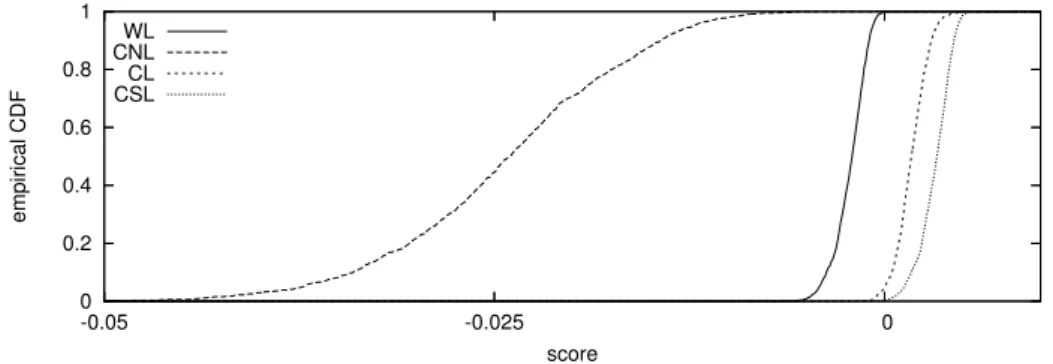
0 0.2 0.4 0.6 0.8 1 -0.05 -0.025 0 empirical CDF score WL CNL CL CSL
Figure 3:Empirical CDFs of mean relative scoresd∗ for the weighted logarithmic (WL) scoring
rule in(4), the censored normal likelihood (CNL) in (8), the conditional likelihood (CL) in (10), and the censored likelihood (CSL) in(11)for series ofP = 2000independent observations from a standard normal distribution. The scoring rules are based on the threshold weight functionw(y) = I(y ≤r)withr =−2.5. The relative score is defined as the score for (correct) standard normal density minus the score for the standardized Student-t(5)density. The graph is based on10,000 replications.
corresponding realizations for P time periods R + 1, . . . , T, we may form the relative scoresdclt+1 = Scl( ˆft;yt+1)−Scl(ˆgt;yt+1)anddcslt+1 = Scsl( ˆft;yt+1)−Scsl(ˆgt;yt+1)and
use these as the basis for computing a Diebold-Mariano type test statistic of the form given in (2).
We revisit the example from the previous section in order to illustrate the properties of the various scoring rules and the associated tests for comparing the accuracy of competing density forecasts. We generate 10,000 independent series of P = 2000 independent observationsyt+1from a standard normal distribution. For each sequence we compute the
mean value of the weighted logarithmic scoring rule in (4), the censored normal likelihood in (8), the conditional likelihood in (10), and the censored likelihood in (11). For the WL scoring rule score we use the threshold weight function w(yt+1) = I(yt+1 ≤ r), where
the threshold is fixed atr = −2.5. The CNL score is used withα = Φ(r), where Φ(·) represents the standard normal CDF. The threshold valuer=−2.5is also used for the CL and CSL scores. Each scoring rule is computed for the (correct) standard normal density
ˆ
ftand the standardized Student-tdensitygˆtwith five degrees of freedom.
Figure 3 shows the empirical CDF of the mean relative scoresd∗, where∗iswl, cnl,
clorcsl. The average WL and CNL scores take almost exclusively negative values, which means that for the weight function considered, on average they attach a lower score to the correct normal distribution than to the Student-t distribution, leading to a bias in the corresponding test statistic towards the incorrect, fat-tailed distribution. The two scoring rules based on partial likelihood both correctly favor the true normal density. The scores of the censored likelihood rule appear to be better at detecting the inadequacy of the
Student-tdistribution, in the sense that its relative scores stochastically dominate those based on the conditional likelihood.
We close this section by noting that the validity of the CL and CSL scoring rules in (10) and (11) does not depend on the particular definition ofVt+1(or weight functionw(Yt+1))
r). This step function is the analogue of the threshold weight function w(Yt+1) used in
the introductory example which motivated our approach. This weight function seems an obvious choice in risk management applications, as the left tail behavior of the density forecast then is of most concern. In other empirical applications of density forecasting, however, the focus may be on a different region of the distribution, leading to alternative weight functions. For example, for monetary policymakers aiming to keep inflation within a certain range, the central part of the distribution may be of most interest, suggesting to defineVt+1asVt+1 =I(rl ≤Yt+1 ≤ru)for given lower and upper boundsrlandru.
4
Smooth weight functions and generalized scoring rules
The conditional and censored likelihood scoring rules in in (10) and (11) with the par-ticular definitions of Vt+1 and corresponding weight functions w(Yt+1)strictly define a
precise region for which the density forecasts are evaluated. This is appropriate in case it is perfectly obvious which specific region is of interest. In practice this may not be so clear-cut, and it may be desirable to define a certain region with less stringent bounds. For example, instead of the threshold weight functionw(Yt+1) = I(Yt+1 ≤ r), we may
consider a logistic weight function of the form
w(Yt+1) = 1/(1 + exp(a(Yt+1−r))) witha >0. (12)
This sigmoidal function changes monotonically from 1 to 0 asYt+1increases, withw(r) = 1
2 and the slope parameteradetermining the speed of the transition. Note that in the limit
as a → ∞, the threshold weight function I(Yt+1 ≤ r) is recovered. In this section
we demonstrate how the partial likelihood scoring rules can be generalized to alternative weight functions, including smooth functions such as (12).
This can be achieved by not takingVt+1 as a deterministic function of Yt+1 as in (9)
but instead allowing Vt+1 to take the value 1with probability w(Yt+1) and0 otherwise,
that is, Vt+1|Yt+1 = ( 1 with probabilityw(Yt+1), 0 with probability1−w(Yt+1), (13) so thatVt+1givenYt+1is a Bernoulli random variable with success probabilityw(Yt+1). In
this more general setting the two-stage experiment can still be thought of as observing only
Vt+1in the first stage andYt+1 in the second stage. The (partial) likelihoods based on the
first and/or second stage information then allow the construction of more general versions of the CL and CSL scoring rules, involving the weight functionw(Yt+1). To see this, recall
that the CL and CSL scoring rules based on the threshold weight function either include the likelihood from the second stage experiment or ignore it, depending on whetherVt+1is
one or zero, respectively. Applying the same recipe in this more general case would lead to arandomscoring rule, depending on the realization of the random variable Vt+1 given
Yt+1. Nevertheless, being likelihood-based scores, these random scores could be used
for density forecast comparison, provided that the same realizations ofVt+1 are used for
both density forecasts under consideration. Random scoring rules would obviously not be very practical, but it is important to notice their validity from an partial likelihood point
of view. In practice we propose to integrate out the random variation by averaging the random scores over the conditional distribution ofVt+1 givenYt+1, which is independent
of the density forecast. The following clarifies how this leads to generalized CL and CSL scoring rules.
Generalized conditional likelihood scoring rule For the first scoring rule, where only the conditional likelihood ofYt+1givenVt+1 = 1is used and no other information on the
realized values ofVt+1, the likelihood givenVt+1is
I(Vt+1 = 1|Yt+1) log ˆ ft(Yt+1) Pfˆ(Vt+1 = 1) ! ,
wherePfˆ(Vt+1 = 1)is the probability thatVt+1 = 1under the assumption thatYt+1 has
densityfˆt. This is a random score function, in the sense that it depends on the random
variable Vt+1. Averaging over the conditional distribution of Vt+1 given Yt+1 leads to
EVt+1|Yt+1;f[I(Vt+1 = 1|Yt+1)] =Pfˆ(Vt+1 = 1|Yt+1) =w(Yt+1), so that the score averaged
overVt+1, givenYt+1, is S( ˆft;Yt+1) =w(Yt+1) log ˆ ft(Yt+1) R∞ −∞ftˆ(x)w(x) dx ! . (14)
It can be seen that this is a direct generalization of the CL scoring rule given in (10), which is obtained by choosingw(Yt+1) =I(Yt+1 ≤r).
Generalized censored likelihood scoring rule As mentioned before, the conditional likelihood scoring rule is based on the conditional likelihood of the second stage experi-ment only. The censored likelihood scoring rule also includes the information revealed by the realized value ofVt+1, that is, the first stage experiment. The log likelihood based on
Yt+1andVt+1 is I(Vt+1 = 1) log ˆft(Yt+1) +I(Vt+1 = 0) log Z ∞ −∞ ˆ f(x)(1−w(x)) dx ,
which, after averaging overVt+1 givenYt+1gives the scoring rule
S( ˆft;Yt+1) =w(Yt+1) log ˆft(Yt+1) + (1−w(Yt+1)) log 1− Z ∞ −∞ ˆ f(x)w(x) dx . (15) The choicew(Yt+1) =I(Yt+1 ≤r)gives the CSL scoring rule as given in (11).
Returning to the simulated example concerning the comparison of the normal and Student-tdensity forecasts, we consider logistic weight functions as given in (12). We fix the center atr = −2.5and vary the slope parameteraamong the values 1, 2, 5, and 10. The integralsR fˆt(y)w(y) dyand
R
ˆ
gt(y)w(y) dyfor the threshold weight function were
determined numerically with the CDF routines from the GNU Scientific Library. For other weight functions the integrals were determined numerically by averagingw(yt+1)over a
large number (106) of simulated random variablesy
0 0.2 0.4 0.6 0.8 1 0 0.01 0.02 0.03 0.04 empirical CDF score (a=1) CL CSL 0 0.2 0.4 0.6 0.8 1 0 0.01 0.02 0.03 0.04 empirical CDF score (a=2) CL CSL 0 0.2 0.4 0.6 0.8 1 0 0.01 0.02 0.03 0.04 empirical CDF score (a=5) CL CSL 0 0.2 0.4 0.6 0.8 1 0 0.01 0.02 0.03 0.04 empirical CDF score (a=10) CL CSL
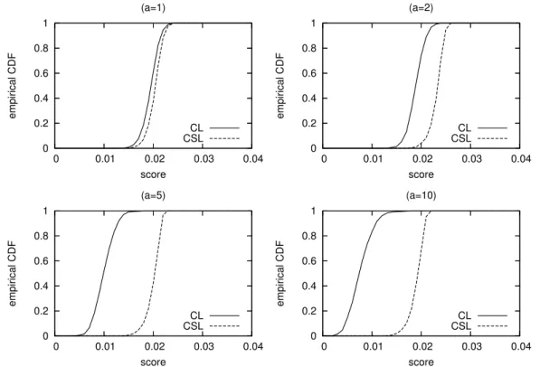
Figure 4: Empirical CDFs of mean relative scoresd∗ for the generalized conditional likelihood
(CL) and censored likelihood (CSL) scoring rules for series ofP = 2000independent observations from a standard normal distribution. The scoring rules are based on the logistic weight function w(y)defined in(12)for various values of the slope parametera. The relative score is defined as the score for (correct) standard normal density minus the score for the standardized Student-t(5) density. The graph is based on10,000replications.
Figure 4 shows the empirical CDFs of the mean relative scoresd∗ obtained with the conditional likelihood and censored likelihood scoring rules for the different values of
a. It can be observed that for the smoothest weight function considered (a = 1) the two score distributions are very similar. The difference between the scores increases as
a becomes larger. Fora = 10, the logistic weight function is already very close to the threshold weight function I(yt+1 ≤r), such that for larger values ofaessentially the same
score distributions are obtained. The score distributions become more similar for smaller values ofabecause, as a → 0,w(yt+1)in (12) converges to a constant equal to 12 for all
values of yt+1, so that w(yt+1)−(1−w(yt+1)) → 0, and moreover R
w(y) ˆft(y) dy =
R
w(y)ˆgt(y) dy → 1
2. Consequently, both scoring rules converge to the unconditional
likelihood (up to a constant factor2) and the relative scoresdcl
t+1anddcslt+1have the limit
1
5
Monte Carlo simulations
In this section we examine the implications of using the weighted logarithmic scoring rule in (4), the censored normal likelihood in (8), the conditional likelihood in (10), and the censored likelihood in (11) for constructing a test of equal predictive ability of two competing density forecasts. Specifically, we consider the size and power properties of the Diebold-Mariano type test as given in (2). The null hypothesis states that the two competing density forecasts have equal expected scores, or
H0 :E[d∗t+1] = 0,
under scoring rule∗, where∗is eitherwl,cnl, clorcsl. We focus on one-sided rejection rates to highlight the fact that some of the scoring rules may favor a wrongly specified density forecast over a correctly specified one. Throughout we use a HAC-estimator for the asymptotic variance of the relative scored∗t+1, that isσˆ2 = ˆγ
0+ 2 PK−1
k=1 akγˆk, where
ˆ
γkdenotes the lag-ksample covariance of the sequence{d∗t+1}
T−1
t=R andak are the Bartlett
weightsak = 1−k/K withK =bP−1/4c, whereP =T −Ris the sample size.
5.1
Size
In order to assess the size properties of the tests a case is required with two competing predictive densities that are both ‘equally (in)correct’. However, whether or not the null hypothesis of equal predictive ability holds depends on the weight functionw(yt+1)that is
used in the scoring rules. This complicates the simulation design, also given the fact that we would like to examine how the behavior of the tests depends on the specific settings of the weight function. For the threshold weight functionw(yt+1) = I(yt+1 ≤r)it appears to
be impossible to construct an example with two different density forecasts having identical predictive ability regardless of the value ofr. We therefore evaluate the size of the tests by focusing on the central part of the distribution using the weight functionw(y) = I(−r ≤
y ≤ r). As mentioned before, in some cases this region of the distribution may be of
primary interest, for instance to monetary policymakers aiming to keep inflation between certain lower and upper bounds. The data generating process (DGP) is taken to be an i.i.d. standard normal distribution, while the two competing density forecasts are normal distributions with means equal to −0.2 and 0.2, and variance equal to 1. In this case, independent of the value ofrthe competing density forecasts have equal predictive ability, as the scoring rules considered here are invariant under a simultaneous reflection about zero of all densities of interest (the true conditional density as well as the two competing density forecasts under consideration). In addition, it turns out that for this combination of DGP and predictive densities, the relative scores d∗t+1 for the WL, CL and CSL rules based onw(y) = I(−r ≤ y ≤ r) are identical. For this weight function the CNL rule takes the form of the last expression in (8), with α = Pt(Yt+1 = 1) = P(−r ≤ Yt+1 ≤
r) = Φ(r)−Φ(−r).
Figure 5 displays one-sided rejection rates (at nominal significance levels of 1, 5 and
10%) of the null hypothesis against the alternative that theN(0.2,1)distribution has better
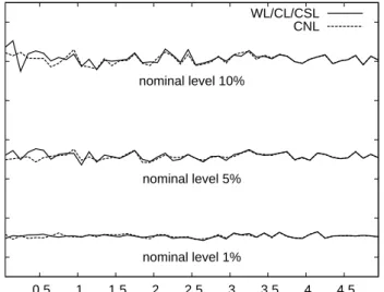
0 0.02 0.04 0.06 0.08 0.1 0.12 0.5 1 1.5 2 2.5 3 3.5 4 4.5 rejection rate threshold r nominal level 1% nominal level 5% nominal level 10% WL/CL/CSL CNL
Figure 5: One-sided rejection rates of the Diebold-Mariano type test statistic of equal predictive
accuracy defined in(2)when using the weighted logarithmic (WL), the censored normal likelihood (CNL), the conditional likelihood (CL), and the censored likelihood (CSL) scoring rules, under the weight functionw(y) =I(−r ≤y ≤r)for sample sizeP = 500, based on 10,000 replications. The DGP is i.i.d. standard normal. The test compares the predictive accuracy ofN(−0.2,1)and N(0.2,1)distributions. The graph shows rejection rates against the alternative that theN(0.2,1) distribution has better predictive ability.
on 10,000 replications). The rejection rates of the tests are quite close to the nominal sig-nificance levels for all values ofr. Unreported results for different values ofP show that this holds even for sample sizes as small as 100 observations. Hence, the size properties of the tests appear to be satisfactory.
It is useful to note that the rejection rates of the CNL scoring rule converge to those based on the WL/CL/CSL scoring rules for large values ofr, when practically the entire distribution is taken into account. This is due to the fact that the ‘unconditional’ scoring rules (which are obtained asr → ∞) all coincide as they become equal to scores based on the unconditional normal likelihood.
5.2
Power
We evaluate the power of the test statistics by performing simulation experiments where one of the competing density forecasts is correct, in the sense that it corresponds with the underlying DGP. In that case the true density always is the best possible one, regardless of the region for which the densities are evaluated, that is, regardless of the weight function used in the scoring rules. Given that our main focus in this paper has been on comparing density forecasts in the left tail, in these experiments we return to the threshold weight functionw(y) =I(y≤r)for the WL, CL and CSL rules. For each value ofrconsidered, the CNL score is used withα= Φ(r), whereΦ(·)represents the standard normal CDF.
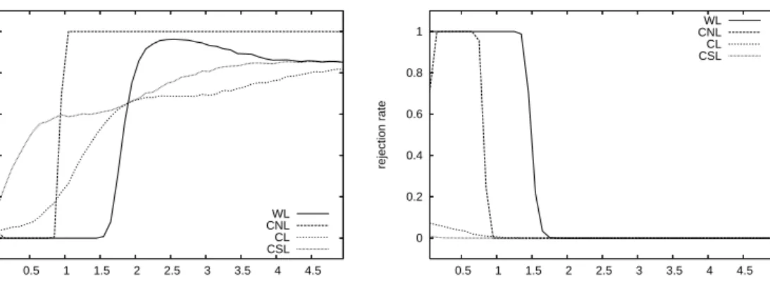
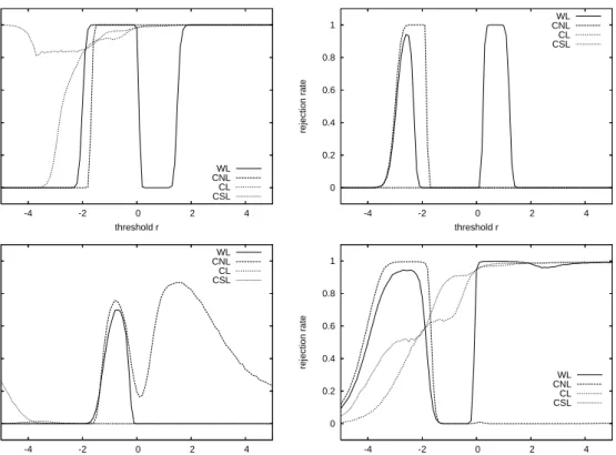
Figures 6 and 7 plot the observed rejection rates for sample sizesP = 500and 2000, respectively (again based on10,000 replications), for data drawn from the standard
0 0.2 0.4 0.6 0.8 1 -4 -2 0 2 4 rejection rate threshold r WL CNL CL CSL 0 0.2 0.4 0.6 0.8 1 -4 -2 0 2 4 rejection rate threshold r WL CNL CL CSL 0 0.2 0.4 0.6 0.8 1 -4 -2 0 2 4 rejection rate threshold r WL CNL CL CSL 0 0.2 0.4 0.6 0.8 1 -4 -2 0 2 4 rejection rate threshold r WL CNL CL CSL
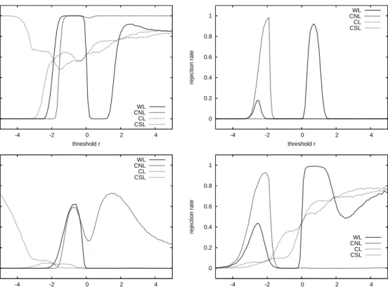
Figure 6: One-sided rejection rates (at nominal significance level 5%) of the Diebold-Mariano
type test statistic of equal predictive accuracy defined in (2)when using the weighted logarithmic (WL), the censored normal likelihood (CNL), the conditional likelihood (CL), and the censored likelihood (CSL) scoring rules, under the threshold weight functionw(y) =I(y ≤r)for sample size P = 500, based on 10,000 replications. For the graphs in the top and bottom rows, the DGP is i.i.d. standard normal and i.i.d. standardized t(5), respectively. The test compares the predictive accuracy of the standard normal and the standardizedt(5)distributions. The graphs in the left (right) panels show rejection rates against superior predictive ability of the standard normal (standardizedt(5)) distribution, as a function of the threshold parameterr.
mal distribution (top row) or the standardized Student-t(5)distribution (bottom row). In both cases, the null hypothesis being tested is equal predictive accuracy of standard nor-mal and standardizedt(5) density forecasts. The left (right) panels in these Figures show rejection rates (at nominal significance level5%) against superior predictive ability of the standard normal (standardizedt(5)) distribution, as a function of the threshold parame-terr. Hence, the top left and bottom right panels report true power (rejections in favor of the correct density), while the top right and bottom left panels report spurious power (rejections in favor of the incorrect density).
Several interesting conclusions emerge from these graphs. First, for large values of the threshold r, the tests based on the WL, CL and CSL scoring rules behave similarly (recall that they become identical when r → ∞) and achieve rejection rates against the correct alternative of around 80% for P = 500and nearly 100% for P = 2000. When the threshold r is fairly large, the CNL-based test has even better power properties for the standard normal DGP, with rejection rates close to 100% already for P = 500. By contrast, it has no power whatsoever in case of the standardized Student-tDGP. The latter
0 0.2 0.4 0.6 0.8 1 -4 -2 0 2 4 rejection rate threshold r WL CNL CL CSL 0 0.2 0.4 0.6 0.8 1 -4 -2 0 2 4 rejection rate threshold r WL CNL CL CSL 0 0.2 0.4 0.6 0.8 1 -4 -2 0 2 4 rejection rate threshold r WL CNL CL CSL 0 0.2 0.4 0.6 0.8 1 -4 -2 0 2 4 rejection rate threshold r WL CNL CL CSL
Figure 7: One-sided rejection rates (at nominal significance level 5%) of the Diebold-Mariano
type test statistic of equal predictive accuracy defined in (2)when using the weighted logarithmic (WL), the censored normal likelihood (CNL), the conditional likelihood (CL), and the censored likelihood (CSL) scoring rules, under the threshold weight functionw(y) =I(y ≤r)for sample size P = 2000, based on 10,000 replications. Specifications of the simulation experiments are identical to Figure 6.
occurs because in this case the normal scoring rule in (6) (which is the limiting case of the CNL-rule whenr→ ∞) has the same expected value for both density forecasts, such that the null hypothesis of equal predictive accuracy actually holds true. To see this, let
ˆ
ft(y)and ˆgt(y) denote theN(0,1)and standardizedt(5) density forecasts, respectively,
with corresponding CDFsFˆtandGˆtand inverse normal transforms Zf,t+1 andZg,t+1. It
then follows that
Et(Zf,t2 +1) = Z ∞ −∞ (yt+1)2gˆt(yt+1) dyt+1 = Vart(Yt+1) = 1, and Et(Zg,t2 +1) = Z ∞ −∞ Φ−1( ˆGt(yt+1)) 2 ˆ gt(yt+1) dyt+1 = Z 1 0 Φ−1(u))2 du= 1, such thatE[dcN
t+1] = 0whenrbecomes large.
Second, the power of the weighted logarithmic scoring rule depends strongly on the threshold parameter r. For the normal DGP, for example, the test has excellent power for values of r larger than 2 and between −2 and 0, but for other threshold values the
-0.03 -0.02 -0.01 0 0.01 0.02 0.03 0.04 0.05 -4 -2 0 2 4 mean score r
Figure 8: Mean relative WL scoreE[dwlt+1]with threshold weight functionw(y) = I(y ≤r)for
the standard normal versus the standardizedt(5)density as a function of the threshold valuer, for the standard normal DGP.
rejection rates against the correct alternative drop to zero. In fact, for these regions of threshold values, we observe substantial rejection rates against the incorrect alternative of superior predictive ability of the Student-tdensity. Comparing Figures 6 and 7 shows that this is not a small sample problem. In fact, the spurious power increases asP becomes larger. To understand the non-monotonous nature of these power curves, we use numerical integration to obtain the mean relative score E[dwl
t+1] for various values of the threshold
r for i.i.d. standard normal data. The results are shown in Figure Figure 8. It can be observed that the mean changes sign several times, in exact accordance with the patterns in the top panels of Figures 6 and 7. Whenever the mean score difference (computed as the score of the standard normal minus the score of the standardizedt(5) density) is positive the associated test has high power, while it has high spurious power for negative mean scores. Similar considerations also explain the spurious power that is found for the CNL scoring rule. Note that in case of the normal DGP, the rejection rates against the incorrect alternative are particularly high for those values ofrthat are most relevant when the interest is in comparing the predictive accuracy for the left tail of the distribution, suggesting that the CNL-rule is not suitable for this purpose.
Third, we find that the tests based on our partial likelihood scoring rules have reason-able power when a considerreason-able part of the distribution is taken into account. For positive threshold values, rejection rates against the correct alternative are between 50 and 80%
forP = 500and close to 100% for the larger sample sizeP = 2000. For the CL-based
test, power declines as r becomes smaller, due to the reduced number of observations falling in the relevant region that is taken into consideration. The power of the CSL-based statistic remains higher, in particular for the normal DGP, suggesting that the additional information concerning the actual coverage probability of the left tail region helps to dis-tinguish between the competing density forecasts. Perhaps even more importantly, we find that the partial likelihood scores do not suffer from spurious power. For both the CL and
0 0.2 0.4 0.6 0.8 1 0.5 1 1.5 2 2.5 3 3.5 4 4.5 rejection rate threshold r WL CNL CL CSL 0 0.2 0.4 0.6 0.8 1 0.5 1 1.5 2 2.5 3 3.5 4 4.5 rejection rate threshold r WL CNL CL CSL
Figure 9: One-sided rejection rates (at nominal significance level 5%) of the Diebold-Mariano
type test statistic of equal predictive accuracy defined in (2)when using the weighted logarithmic (WL), the censored normal likelihood (CNL), the conditional likelihood (CL), and the censored likelihood (CSL) scoring rules, under the weight functionw(y) =I(−r≤y≤r)for sample size P = 500, based on 10,000 replications. The DGP is i.i.d. standard normal. The graphs on the left and right show rejection rates against better predictive ability of the standard normal distribution compared to the standardizedt(5)distribution andvice versa.
CSL rules, the rejection rates against the incorrect alternative remain below the nominal significance level of 5%. The only exception occurs for the i.i.d. standardizedt(5) DGP, where the CSL-based exhibits spurious power for small values of the threshold parameter
r when P = 500. Comparing the bottom-left panels of Figures 6 and 7 suggests that
this is a small sample problem though, as the rejection rates decline considerably when increasing the number of forecasts toP = 2000.
Finally, to study the power properties of the tests when they are used to compare density forecasts on the central part of the distribution, we perform the same simulation experiments but using the weight functionw(y) = I(−r ≤y ≤ r)in the various scoring rules. Only a small part of these results are included here; full details are available upon re-quest. Figure 9 shows rejection rates obtained for an i.i.d. standard normal DGP, when we test the null of equal predictive ability of theN(0,1)and standardizedt(5) distributions against the alternative that either of these density forecasts has better predictive ability, for sample sizeP = 500. The left panel shows rejection rates against better predictive per-formance of the (correct)N(0,1)density, while the right panel shows the spurious power, that is rejection rates against better predictive performance of the (incorrect) standardized
t(5)distribution. Clearly, all tests have high power, provided that the observations from a sufficiently wide interval(−r, r)are taken into account. It can also be observed that the tests based on WL and CNL scores suffer from a large spurious power even for quite rea-sonable values ofr, while the spurious power for the tests based on the partial likelihood scores remains smaller than the nominal level (5%).
6
Empirical illustration
We examine the empirical relevance of our partial likelihood-based scoring rules in the context of the evaluation of density forecasts for daily stock index returns. We consider
S&P 500 log-returns yt = ln(Pt/Pt−1), where Pt is the closing price on dayt, adjusted
for dividends and stock splits. The sample period runs from January 1, 1980 until March 14, 2008, giving a total of 7115 observations (source: Datastream).
For illustrative purposes we define two forecast methods based on GARCH models in such a way that a priori one of the methods is expected to be superior to the other. Examining a large variety of GARCH specifications for forecasting daily US stock index returns, Baoet al. (2007) conclude that the accuracy of density forecasts depends more on the choice of the distribution of the standardized innovations than on the choice of the volatility specification. Therefore, we differentiate our forecast methods in terms of the innovation distribution, while keeping identical specifications for the conditional mean and the conditional variance. We consider an AR(5) model for the conditional mean return together with a GARCH(1,1) model for the conditional variance, that is
yt=µt+εt=µt+
p
htηt,
where the conditional meanµtand the conditional variancehtare given by
µt=ρ0+ 5 X j=1 ρjyt−j, ht=ω+αε2t−1+βht−1,
and the standardized innovationsηtare i.i.d. with mean zero and variance one.
Following Bollerslev (1987), a common finding in empirical applications has been that GARCH models with a normal distribution forηtare not able to fully account for the
kurtosis observed in stock returns. We therefore concentrate on leptokurtic distributions for the standardized innovations. Specifically, for one forecast method the distribution of
ηtis specified as a (standardized) Student-tdistribution withνdegrees of freedom, while
for the other forecast method we use the (standardized) Laplace distribution. Note that for the Student-tdistribution the degrees of freedomν is a parameter that is to be estimated. The degrees of freedom directly determines the value of the excess kurtosis of the stan-dardized innovations, which is equal to6/(ν−4)(assumingν >4). Due to its flexibility, the Student-tdistribution has been widely used in GARCH modeling (see e.g. Bollerslev (1987), Baillie and Bollerslev (1989)). The standardized Laplace distribution provides a more parsimonious alternative with no additional parameters to be estimated and has been applied in the context of conditional volatility modeling by Granger and Ding (1995) and Mittniket al. (1998)). The Laplace distribution has excess kurtosis of3, which exceeds the excess kurtosis of the Student-t(ν) distribution for ν > 6. Because of the greater flexibility in modeling kurtosis, we may expect that the forecast method with Student-t
innovations gives superior density forecasts relative to the Laplace innovations. This is indeed indicated by results in Bao et al. (2007), who evaluate these density forecasts ‘unconditionally’, that is, not focusing on a particular region of the distribution.
Our evaluation of the two forecast methods is based on their one-step ahead density forecasts for returns, using a rolling window scheme for parameter estimation. The width of the estimation window is set toR = 2000observations, so that the number of out-of-sample observations is equal toP = 5115. For comparing the density forecasts’ accuracy
we use the Diebold-Mariano type test based on the weighted logarithmic scoring rule in (4), the censored normal likelihood in (8), the conditional likelihood in (10), and the censored likelihood in (11). We concentrate on the left tail of the distribution by using the threshold weight functionw(yt+1) = I(yt+1≤rt)for the WL, CL and CSL scoring rules.
We consider two time-varying thresholds rt, that are determined as the one-day
Value-at-Risk estimates at the 95% and 99% level based on the corresponding quantiles of the empirical CDF of the return observations in the relevant estimation window. For the CNL scoring rule in (8) we use the corresponding valuesα= 0.05and 0.01, respectively. The score differenced∗t+1is computed by subtracting the score of the GARCH-Laplace density forecast from the score of the GARCH-tdensity forecast, such that positive values ofd∗t+1
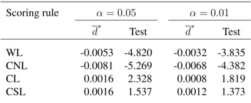
indicate better predictive ability of the forecast method based on Student-tinnovations. Table 1 shows the average score differences d∗ with the accompanying tests of equal predictive accuracy as in (2), where we use a HAC estimator for the asymptotic variance ˆ
σ2 to account for serial dependence in the d∗
t+1 series. The results clearly demonstrate
that different conclusions follow from the different scoring rules. For both choices of the thresholdrtthe WL and CNL scoring rules suggest superior predictive ability of the
forecast method based on Laplace innovations. By contrast, the CL scoring rule suggests that the performance of the GARCH-t density forecasts is superior. The CSL scoring rule points towards the same conclusion as the CL rule, although the evidence for better predictive ability of the GARCH-tspecification is somewhat weaker. In the remainder of this section we seek to understand the reasons for these conflicting results, and explore the consequences of selecting either forecast method for risk management purposes. In addition, this allows us to obtain circumstantial evidence that shows which of the two competing forecast methods is most appropriate.
For most estimation windows, the degrees of freedom parameter in the Student-t dis-tribution is estimated to be (slightly) larger than 6, such that the Laplace disdis-tribution im-plies fatter tails than the Student-tdistribution. Hence, it may very well be that the WL and CNL scoring rules indicate superior predictive ability of the Laplace distribution sim-ply because this density has more probability mass in the region of interest, that is, the problem that motivated our analysis in the first place. To see this from a slightly differ-ent perspective, we compute one-day 95% and 99% Value-at-Risk (VaR) and Expected Shortfall (ES) estimates as implied by the two forecast methods. The 100×(1−α)% Value-at-Risk is determined as theα-th quantile of the density forecastftˆ, that is, through Pf ,tˆ
Yt+1 ≤VaRf ,tˆ (α)
=α. The Expected Shortfall is defined as the conditional mean return given that Yt+1 ≤ VaRf ,tˆ (α), that isESf ,tˆ (α) = Ef ,tˆ
Yt+1|Yt+1 ≤VaRf ,tˆ (α)
. Figure 10 shows the VaR estimates against the realized returns. We observe that typically the VaR estimates based on the Laplace innovations are more extreme and, thus, imply fatter tails than the Student-tinnovations. The same conclusion follows from the sample averages of the VaR and ES estimates, as shown in Table 2.
The VaR and ES estimates also enable us to assess which of the two innovation distri-butions is the most appropriate in a different way. For that purpose, we first of all compute the frequency of 95% and 99% VaR violations, which should be close to 0.05 and 0.01, respectively, if the innovation distribution is correctly specified. We compute the likeli-hood ratio (LR) test of correct unconditional coverage (CUC) suggested by Christoffersen
Table 1:Average score differences and tests of equal predictive accuracy Scoring rule α= 0.05 α= 0.01 d∗ Test d∗ Test WL -0.0053 -4.820 -0.0032 -3.835 CNL -0.0081 -5.269 -0.0068 -4.382 CL 0.0016 2.328 0.0008 1.819 CSL 0.0016 1.537 0.0012 1.373 Note: The table presents the average score differenced∗for the weighted logarithmic (WL) scoring rule in (4), the censored nor-mal likelihood (CNL) in (8), the conditional likelihood (CL) in (10), and the censored likelihood (CSL) in (11). The WL, CL and CSL scoring rules are based on the threshold weight function
w(yt+1) =I(yt+1≤rt), wherertis theα-th quantile of the
em-pirical (in-sample) CDF, whereα= 0.01or 0.05. These values forαare also used for the CNL scoring rule. The score difference
dt+1 is computed for density forecasts obtained from an
AR(5)-GARCH(1,1) model with (standardized) Student-t(ν)innovations relative to the same model but with Laplace innovations, for daily S&P500 returns over the evaluation period December 2, 1987 – March 14, 2008.
Figure 10:Daily S&P 500 log-returns (black) for the period December 2, 1987 – March 14, 2008
and out-of-sample 95% and 99% VaR forecasts derived from the AR(5)-GARCH(1,1) specification using Student-tinnovations (light gray) and Laplace innovations (dark gray).
Table 2:Value-at-Risk and Expected Shortfall characteristics α = 0.05 α= 0.01 t(ν) Laplace t(ν) Laplace Average VaR −0.0149 −0.0162 −0.0247 −0.0279 Coverage(yt≤VaRt) 0.0532 0.0407 0.0104 0.0055 CUC (p-value) 0.3019 0.0016 0.7961 0.0004 IND (p-value) 0.0501 0.3823 0.5809 0.5788 CCC (p-value) 0.0861 0.0046 0.8304 0.0015 Average ES −0.0209 −0.0235 −0.0312 −0.0351 McNeil-Frey (test stat.) 1.0678 0.0851 1.0603 1.9730 McNeil-Frey (p-value) 0.2856 0.9322 0.2890 0.0485 Note: The average VaRs reported are the observed average5% and1%quantiles of the density forecasts based on the GARCH model witht(ν)and Laplace innovations, respectively. The coverages correspond with the observed fraction of returns below the respective VaRs, which ideally would coincide with the nominal rateα. The rows labeled CUC, IND and CCC providep-values for Christoffersen’s (1998) tests for cor-rect unconditional coverage, independence of VaR violations, and corcor-rect conditional coverage, respectively. The average ES values are the expected shortfalls (equal to the conditional mean return, given a realization below the predicted VaR) based on the dif-ferent density forecasts. The bottom two rows report McNeil-Frey test statistics and correspondingp-values for evaluating the expected shortfall estimatesESf ,tˆ (α).
(1998) to determine whether the empirical violation frequencies differ significantly from these nominal levels. Additionally, we use Christoffersen’s (1998) LR tests of indepen-dence of VaR violations (IND) and for correct conditional coverage (CCC). Define the indicator variablesIf ,tˆ +1(yt+1 ≤VaRf ,tˆ (α))forα = 0.05and0.01, which take the value
1if the condition in brackets is satisfied and 0 otherwise. Independence of the VaR vi-olations is tested against a first-order Markov alternative, that is, the null hypothesis is given by H0 : E(If ,tˆ +1|If ,tˆ ) = E(If ,tˆ +1). In words, we test whether the probability of
observing a VaR violation on dayt+ 1is affected by observing a VaR violation on day
t or not. The CCC test simultaneously examines the null hypotheses of correct uncon-ditional coverage and of independence, with the CCC test statistic simply being the sum of the CUC and IND LR statistics. For evaluating the adequacy of the Expected Short-fall estimates ESf ,tˆ (α) we employ the test suggested by McNeil and Frey (2000). For
every returnytthat falls below theVaRf ,tˆ (α)estimate, define the standardized ‘residual’
et+1 = (yt+1−ESf ,tˆ (α))/ht+1, whereht+1 is the conditional volatility forecast obtained
from the corresponding GARCH model. Under the null of correct specification, the ex-pected value ofet+1is equal to zero, which can easily be assessed by means of a two-sided
t-test with HAC variance estimator.
The results reported in Table 2 show that the empirical VaR violation frequencies are very close to the nominal levels for the Student-tinnovation distribution. For the Laplace distribution, they are considerably lower. This is confirmed by the CUC test, which con-vincingly rejects the null of correct unconditional coverage for the Laplace distribution but
not for the Student-tdistribution. The null hypothesis of independence is not rejected in any of the cases at the 5% significance level. Finally, the McNeil and Frey (2000) test does not reject the adequacy of the 95% ES estimates for either of the two distributions, but it does for the 99% ES estimates based on the Laplace innovation distribution. In sum, the VaR and ES estimates suggest that the Student-tdistribution is more appropriate than the Laplace distribution, confirming the density forecast evaluation results obtained with the scoring rules based on partial likelihood. In terms of risk management, using the GARCH-Laplace forecast method would lead to larger estimates of risk than the GARCH-tforecast method. This, in turn, could result in suboptimal asset allocation and ‘over-hedging’.
7
Conclusions
In this paper we have developed scoring rules based on partial likelihood functions for evaluating the predictive ability of competing density forecasts. It was shown that these scoring rules are particularly useful when the main interest lies in comparing the density forecasts’ accuracy for a specific region, such as the left tail in financial risk management applications. Conventional scoring rules based on KLIC or censored normal likelihood are not suitable for this purpose. By construction they tend to favor density forecasts with more probability mass in the region of interest, rendering the tests of equal predictive ac-curacy biased towards such densities. Our novel scoring rules based on partial likelihood functions do not suffer from this problem.
Monte Carlo simulations were used to demonstrate that the conventional scoring rules may indeed give rise to spurious rejections due to the possible bias in favor of an incorrect density forecast. The simulation results also showed that this phenomenon is virtually non-existent for the new scoring rules, and where present, diminishes quickly upon in-creasing the sample size.
In an empirical application to S&P 500 daily returns we investigated the use of the various scoring rules for density forecast comparison in the context of financial risk man-agement. It was shown that the scoring rules based on KLIC and censored normal like-lihood functions and the newly proposed partial likelike-lihood scoring rules can lead to the selection of different density forecasts. The density forecasts preferred by the partial like-lihood scoring rules appear to be more appropriate as they were found to result in more accurate estimates of Value-at-Risk and Expected Shortfall.
![Figure 8: Mean relative WL score E[d wl t+1 ] with threshold weight function w(y) = I(y ≤ r) for the standard normal versus the standardized t(5) density as a function of the threshold value r, for the standard normal DGP.](https://thumb-us.123doks.com/thumbv2/123dok_us/483511.2557216/21.892.301.635.133.385/relative-threshold-function-standard-standardized-function-threshold-standard.webp)