University of Toronto
Department of Economics
April 03, 2008
By Chun Liu and John M Maheu
Forecasting Realized Volatility: A Bayesian Model Averaging
Approach
Forecasting Realized Volatility: A Bayesian Model
Averaging Approach
∗
Chun Liu
School of Economics and Management
Tsinghua University
John M. Maheu
Dept. of Economics
University of Toronto
This version: March 2008
Abstract
How to measure and model volatility is an important issue in finance. Recent research uses high frequency intraday data to construct ex post measures of daily volatility. This paper uses a Bayesian model averaging approach to forecast realized volatility. Candidate models include autoregressive and heterogeneous autoregres-sive (HAR) specifications based on the logarithm of realized volatility, realized power variation, realized bipower variation, a jump and an asymmetric term. Applied to equity and exchange rate volatility over several forecast horizons, Bayesian model averaging provides very competitive density forecasts and modest improvements in point forecasts compared to benchmark models. We discuss the reasons for this, including the importance of using realized power variation as a predictor. Bayesian model averaging provides further improvements to density forecasts when we move away from linear models and average over specifications that allow for GARCH effects in the innovations to log-volatility.
∗We are grateful to Olsen Financial Technologies GmbH, Zurich, Switzerland for making the high frequency FX data available. We thank the co-editor, Tim Bollerslev, and three anonymous referees for many helpful comments. We thank Tom McCurdy who contributed to the preparation of the data used in this paper, and the helpful comments from Doron Avramov, Chuan Goh, Raymond Kan, Mark Kamstra, Gael Martin, Alex Maynard, Tom McCurdy, Angelo Melino, Neil Shephard and participants of the Far Eastern Meetings of the Econometric Society, Beijing, and China International Conference in Finance, Xi’an. Maheu thanks the SSHRCC for financial support.
1
Introduction
How to measure and model volatility is an important issue in finance. Volatility is latent and not observed directly. Traditional approaches are based on parametric models such as GARCH or stochastic volatility models. In recent years, a new approach to model-ing volatility dynamics has become very popular which uses improved measures of ex post volatility constructed from high frequency data. This new measure is called real-ized volatility (RV) and is discussed formally by Andersen, Bollerslev, Diebold and Labys (2001), Andersen, Bollerslev, Diebold and Ebens (2001) and Barndorff-Nielsen and Shep-hard (2002a,2002b).1 RV is constructed from the sum of high frequency squared returns
and is a consistent estimator of integrated volatility plus a jump component for a broad class of continuous time models. In contrast to traditional measures of volatility, such as squared returns, realized volatility is more efficient. Recent work has demonstrated the usefulness of this approach in finance. For example, Bollerslev and Zhou (2002) use real-ized volatility to simplify the estimation of stochastic volatility diffusions, while Fleming, Kirby and Ostdiek (2003) demonstrate that investors who use realized volatility improve portfolio decisions.
This paper investigates Bayesian model averaging for models of volatility and con-tributes to a growing literature that investigates time series models of realized volatility and their forecasting power. Recent contributions include Andersen, Bollerslev, Diebold and Labys (2003), Andersen, Bollerslev and Meddahi (2005), Andreou and Ghysels (2002), Koopman, Jungbacker and Hol (2005), Maheu and McCurdy (2002), and Martens, Dijk and Pooter (2004). These papers concentrate on pure time series specifications of RV, however, there may be benefits to model averaging and including additional volatility proxies.
Barndorff-Nielsen and Shephard (2004) have defined several new measures of volatility, and associated estimators. Realized power variation (RPV), is constructed from the sum of powers of the absolute value of high frequency returns. This is a consistent estimator of the integral of the spot volatility process raised to a positive power (integrated power variation). Realized bipower variation, which is defined as the sum of the products of intraday adjacent returns, is a consistent estimator of integrated volatility.
There are several reasons why RPV may improve the forecasting of volatility. Barndorff-Nielsen and Shephard (2004) show that power variation is robust to jumps. Jumps are generally large outliers that may have a strong effect on model estimates and forecasts. Second, the absolute value of returns displays stronger persistence than squared returns (Ding, Granger and Engle (1993)), and therefore may provide a better signal for volatil-ity. Third, Forsberg and Ghysels (2007), Ghysels, Santa-Clara and Valkanov (2006) and Ghysels and Sinko (2006) demonstrate that absolute returns (power variation of order 1) enhance volatility forecasts. Forsberg and Ghysels (2007) argue that the gains are due to the higher predictability, smaller sampling error and a robustness to jumps.2
1Earlier use of realized volatility includes French, Schwert and Stambaugh (1987), Schwert (1989),
and Hsieh (1991).
2Other papers that have used realized power variation include Ghysels et al. (2007). A range of
Building on this work, we show empirically for data from equity and foreign exchange markets that persistence is highest for realized power variation measures. The correlation between realized volatility and lags of realized power variation as a function of the order
p, is maximized for 1.0≤p≤1.5, and notp= 2, which corresponds to realized volatility. Compared with models using just realized volatility, daily squared returns or the intraday range, we find that power variation and bipower variation can provide improvements.
These observations motivate a wide range of useful specifications using realized volatil-ity, power variation of several orders, bipower variation, a jump and an asymmetric term. We focus on the benefits of Bayesian model averaging (BMA) for forecasts of daily, weekly and biweekly average realized volatility. BMA is constructed from autoregressive type parameterizations and variants of the heterogeneous autoregressive (HAR-log) model of Corsi (2004) and Andersen et al. (2007) extended to include different regressors. Choos-ing one model ignores model uncertainty, understates the risk in forecastChoos-ing and can lead to poor predictions (Hibon and Evgeniou (2004)).3 BMA combines individual model
fore-casts based on their predictive record. Therefore, models with good predictions receive large weights in the Bayesian model average.
We compare models’ density forecasts using the predictive likelihood. The predictive likelihood contains the out-of-sample prediction record of a model, making it the central quantity of interest for model evaluation (Geweke and Whiteman (2005)). The empirical results show BMA to be consistently ranked at the top among all benchmark models, including a simple equally weighted model average. Considering all data series and fore-cast horizons, the BMA is the dominate model. Although there are substantial gains in BMA based on density forecasts, point forecasts using the predictive mean show smaller improvements.
The importance of GARCH dynamics in time series models of log-realized-volatility has been documented by Bollerslev et al. (2007). We find that Bayesian model averaging provides further improvements to density forecasts when we move away from linear models and average over specifications that allow for GARCH effects. For example, it provides improvements relative to a benchmark HAR-log-GARCH model for daily density forecasts. There are two main reasons why BMA delivers good performance. First, we show that no single specification dominates across markets and forecast horizons. For each market and forecast horizon there is considerable model uncertainty in all our applica-tions. In other words, there is model risk associated with selecting any individual model. The ranking of individual models can change dramatically over data series and forecast horizons. Bayesian model averaging provides an optimal way to combine this informa-tion.4 The second reason, is that based on the predictive likelihood, including RPV terms can dramatically improve forecasting power. Although specifications with RPV terms also display considerable model uncertainty, BMA gives them larger weights when they perform well.
3Recent examples of Bayesian model averaging in a macroeconomic context include Fern´andez, Ley,
and Steel (2001), Jacobson and Karlsson (2004), Koop and Potter (2004), Pesaran and Zaffaroni(2005) and Wright (2003).
4Based on a logarithmic scoring rule, averaging over all the models provides superior predictive ability
The relative forecast performance of the specifications that enter the model average is ordered as follows. As a group, models with RPV regressors deliver forecast improvements. Bipower variation delivers relatively smaller improvements over models with only realized volatility regressors. A realized jump term which is constructed from bipower variation is important in all model formulations.
This paper is organized as follows. Section 2 discusses the econometric issues for Bayesian estimation and forecasting. Section 3 reviews the theory behind the improved volatility measures: realized volatility, realized power variation and realized bipower vari-ation. Section 4 details the data and the adjustment to RV and realized bipower variation in the presence of market microstructure noise. The selection of regressors is discussed in Section 5. Section 6 presents the different configurations that enter the model averaging while Section 7 discusses forecasting results as well as the role of realized power variation, and the performance of BMA when allowing for GARCH effects. The last section con-cludes. An appendix explains how to calculate the marginal likelihood, and describes the algorithm to estimate volatility models with GARCH innovations.
2
Econometric Issues
2.1
Bayesian Estimation and Gibbs Sampling
To conduct formal model comparisons and model averaging we use Bayesian estimation methods. All the models we consider take the form of a standard normal linear regression
yt=Xt−1β+²t, ²t∼N(0, σ2). (1)
In the following let YT = [y1, ..., yT]0 be a vector of size T, and X a T x k matrix of regressors with row Xt−1. Inference focuses on the posterior density. By Bayes rule, the
prior distributionp(β, σ2), given data and a likelihood functionp(YT|β, σ2), is updated to the posterior distribution,5
p(β, σ2|YT) =
p(YT|β, σ2)p(β, σ2) ∫ ∫
p(YT|β, σ2)p(β, σ2)dβdσ2
. (2)
We specify independent conditionally conjugate priors for β ∼ N(b0, B0), and σ2 ∼
IG(v0
2,
s0
2
)
, where IG(·,·) denotes the inverse gamma distribution. Although the pos-terior is not a well known distribution we can obtain samples from the pospos-terior based on a Gibbs sampling scheme. Specifically, the conditional distributions used in sampling are
β|YT, σ2 ∼ N(M, V), where M =V ( σ−2X0Y T +B0−1b0 ) , V = (σ−2X0X+B−1 0 )−1 , and σ2|Y T, β∼IG (v 2, s 2 ) wherev =T +v0, s= (YT −Xβ)0(YT −Xβ) +s0.
Good introductions to Gibbs sampling and Markov chain Monte Carlo (MCMC) meth-ods can be found in Chib (2001) and Geweke (2005). Formally, Gibbs sampling involves the following steps. Select a starting value, β(0) and σ2(0), and number of iterations N,
then iterate on
• sampleβ(i) ∼p(β|Y
T, σ2(i−1)).
• sampleσ2(i)∼p(σ2|Y
T, β(i)).
Repeating these steps N times produces the draws {θ(i)}N
i=1 = {β
(i), σ2(i)}N i=1. To
eliminate the effect of starting values, we drop the firstN0 draws and collect the nextN.
For a sufficiently large sample this Markov chain converges to draws from the station-ary distribution which is the posterior distribution. A simulation consistent estimate of features of the posterior density can be obtained by sample averages. For example, the posterior mean of the functiong(·) can be estimated as
E[g(θ)|YT]≈ 1 N N ∑ i=1 g(θ(i))
which converges almost surely to E[g(θ)|YT] as N goes to infinity.
In this paper we compare forecasts of models based on the predictive mean. The predictive mean is computed as
E[yT+1|YT]≈ 1 N N ∑ i=1 XTβ(i). (3)
As a new observation arrives the posterior is updated through a new round of Gibbs sampling and a forecast for yT+2 can be calculated.
2.2
Model Comparison
There is a long tradition in the Bayesian literature of comparing models based on pre-dictive distributions (Box (1980), Gelfand and Dey (1994), and Gordon (1997)). In a similar fashion to the Bayes factor which is based on all the data, we can compare the performance of models on a specific out-of-sample period. Given the information set
Ys−1 ={y1, ..., ys−1}, the predictive likelihood (Geweke (1995,2005)) for model Mk is de-fined for the data ys, ..., yt, s < t as
p(ys, ..., yt|Ys−1, Mk) = ∫
p(ys, ..., yt|θk, Ys−1, Mk)p(θk|Ys−1, Mk)dθk, (4) where p(ys, ..., yt|θk, Ys−1, Mk) is the conditional data density given Ys−1. The predictive
likelihood is the predictive density evaluated at the realized outcomeys, ..., yt. Note that integration is performed with respect to the posterior distribution based on the dataYs−1.
Ifs = 1, this is the marginal likelihood and the above equation changes to
p(y1, ..., yt|Mk) = ∫
p(y1, ..., yt|θk, Mk)p(θk|Mk)dθk, (5) wherep(y1, ..., yt|θk, Mk) is the likelihood and p(θk|Mk) the prior for model Mk.
The predictive likelihood contains the out-of-sample prediction record of a model, making it the central quantity of interest for model evaluation (Geweke and Whiteman (2005)). For example, (4) is simply the product of the individual predictive likelihoods,
p(ys, ..., yt|Ys−1, Mk) = t ∏
j=s
p(yj|Yj−1, Mk), (6)
where each of the terms p(yj|Yj−1, Mk) has parameter uncertainty integrated out. The relative value of density forecasts can be compared using the realized data ys, ..., yt with the predictive likelihoods for two or more models.
The Bayesian approach allows for the comparison and ranking of models by predictive Bayes factors. Suppose we have K different models denoted by Mk, k = 1, . . . , K, then the predictive Bayes factor for the datays, ..., yt and models M0 versus M1 is
P BF01 =p(ys, ..., yt|Ys−1, M0)/p(ys, ..., yt|Ys−1, M1).
This summarizes the relative evidence for model M0 versus M1. An advantage of using
Bayes factors for model comparison is that they automatically include Occam’s razor effect in that they penalize highly parameterized models that do not deliver improved predictive content. For the advantages of the use of Bayes factors see Koop and Potter (1999). Kass and Raftery (1995) recommend considering twice the logarithm of the Bayes factor for model comparison, as it has the same scaling as the likelihood ratio statistic.6 In this
paper we report estimates of the predictive likelihood corresponding to an out-of-sample period in which point forecasts are also investigated.
2.3
Calculating the Predictive Likelihood
The previous results require the calculation of the predictive likelihood for each model. Following Geweke (1995), each of the individual terms of the right hand side of (6) can be estimated consistently from the Gibbs sampler output as
p(yj|Yj−1, Mk)≈ 1 N N ∑ i=1 p ( yj|θ(ki), Yj−1, Mk ) , (7) where θ(ki) = {βk(i), σk2(i)}. p(yj|θ (i)
k , Yj−1, Mk) in the context of (1) denotes the normal density with mean Xj−1βk(i) and variance σk2(i), evaluated at yj, and the Gibbs sampler draws are obtained based on the information set Yj−1.
2.4
Bayesian Model Averaging
In a Bayesian context it is straightforward to entertain many models and combine their information and forecasts in a consistent fashion. There are several justifications for
6Kass and Raftery suggest a rule-of-thumb of support forM
0based on 2 logP BF01: 0 to 2 not worth
Bayesian model averaging. Min and Zellner (1993) show that the model average minimizes the expected predicted squared error when the models are exhaustive, while it is superior based on a logarithmic scoring rule (Raftery et al. (1997)). For an introduction to Bayesian model averaging see Hoeting et al. (1999) and Koop (2003). The probability of model Mk given the information set YT is7,
p(Mk|YT) =
p(YT|Mk)p(Mk) ∑K
i=1p(YT|Mi)p(Mi)
(8)
where K is the total number of models. In this equation, p(Mk) is the prior model probability, and p(YT|Mk) is the marginal likelihood. In the context of recursive out-of-sample forecasts, it is more convenient to work with a period-by-period update to model probabilities. Given YT−1, after observing a new observation yT, we update as
p(Mk|yT, YT−1) =
p(yT|YT−1, Mk)p(Mk|YT−1)
∑K
i=1p(yT|YT−1, Mi)p(Mi|YT−1)
. (9)
p(yT|YT−1, Mk) is the predictive likelihood value for modelMk based on informationYT−1,
and can be estimated by (7). p(Mk|YT−1) is last period’s model probability.
The predictive likelihood for BMA is an average of each of the individual model pre-dictive likelihoods, p(yT+1|YT) = K ∑ i=1 p(yT+1|YT, Mi)p(Mi|YT), (10) where each model’s predictive density is estimated from (7). Similarly, the predictive mean of yT+1 is, E[yT+1|YT] = K ∑ i=1 E[yT+1|YT, Mi]p(Mi|YT), (11) which is a weighted average, using the model probabilities, of model specific predictive means.
3
Realized Volatility, Power Variation and Bipower
Variation
A good discussion of the class of special semi-martingales, which are stochastic processes consistent with arbitrage-free prices can be found in Andersen, Bollerslev, Diebold and Labys (2003). These processes allow for a wide range of dynamics including jumps in the mean and variance process as well as long memory.
For illustration, consider the following logarithmic price process:
dp(t) =µ(t)dt+σ(t)dW(t) +κ(t)dq(t), 0≤t ≤T, (12)
7Note that (8) can be written asp(M
k)/
∑K
i=1BFikp(Mi), whereBFik≡p(YT|Mi)/p(YT|Mk) is the Bayes factor for modeli versus modelk.
where µ(t) is a continuous and locally bounded variation process, σ(t) is the stochastic volatility process, W(t) denotes a standard Brownian motion,dq(t) is a counting process with dq(t) = 1 corresponding to a jump at time t and dq(t) = 0 corresponding to no jump, a jump intensityλ(t), and κ(t) refers to the size of a realized jump. The increment inquadratic variation from timet to t+ 1 is defined as
QVt+1 = ∫ t+1 t σ2(s)ds+ ∑ t<s≤t+1,dq(s)=1 κ2(s) (13)
where the first component, called integrated volatility, is from the continuous component of (12), and the second term is the contribution from discrete jumps. Barndorff-Nielsen and Shephard (2004) consider integrated power variation of order p defined as
IP Vt+1(p) =
∫ t+1
t
σp(s)ds (14)
where 0< p ≤2. ClearlyIP Vt+1(2) is integrated volatility.
To consider estimation of these quantities, we normalize the daily time interval to unity and divide it into m periods. Each period has length ∆ = 1/m. Then define the ∆ period return as rt,j =p(t+j∆)−p(t+ (j −1)∆), j = 1, ..., m. Note that the daily return is rt =
∑m
j=1rt,j. Barndorff-Nielsen and Shephard (2004) introduce the following estimator called realized power variation of order p defined as
RP Vt+1(p) =µ−p1∆ 1−p/2 m ∑ j=1 |rt,j|p, (15) where µp =E|µ|p = 2p/2 Γ( 1 2(p+1))
Γ(12) for p >0 where µ∼ N(0,1). Note that for the special
case of p= 2 equation (15) becomes
RP Vt+1(2) =
m ∑
j=1
rt,j2 ≡RVt+1 (16)
and we have the realized volatility, RVt+1, estimator discussed in Andersen, Bollerslev,
Diebold and Labys (2001), Barndorff-Nielsen and Shephard (2002b), and Meddahi (2002). To avoid confusion we refer to RP Vt+1(p) for p < 2 as realized power variation, and to
(16) asRVt+1.
Another estimator considered in Barndorff-Nielsen and Shephard (2004) is realized bipower variation which is,
RBPt+1 ≡µ−12 m ∑ j=2 |rt,j−1||rt,j|, (17) whereµ1 = √ 2/π.
As shown by the papers discussed above, as m→ ∞ RP Vt+1(p) p →IP Vt+1(p) = ∫ t+1 t σp(s)ds for p∈(0,2) (18) RVt+1 p →QVt+1 = ∫ t+1 t σ2(s)ds+∑κ2(s) (19) RBPt+1 p →IP Vt+1(2) = ∫ t+1 t σ2(s)ds. (20)
Note that the asymptotics operate within a fixed time interval by sampling more fre-quently. RV converges to quadratic variation, and the latter measures the ex post varia-tion of the process regardless of the model or informavaria-tion set. Therefore, realized volatility is the relevant quantity to focus on the modeling and forecasting of volatility. For further details on the relationship between RV and the second moments of returns see Andersen, Bollerslev, Diebold and Labys (2003), Barndorff-Nielsen and Shephard (2002a,2005) and Meddahi (2003).
From these results, it follows that the jump component in QVt+1 can be estimated by
RVt+1 −RBPt+1. RP Vt+1(p) for p ∈ (0,2) and RBPt+1 are robust to jumps. Forsberg
and Ghysels (2007), Ghysels, Santa-Clara and Valkanov (2006) and Ghysels and Sinko (2006) have found that absolute returns (power variation of order 1) improve volatility forecasting using criterions such as adjustedR2 and Mean Squared Error. They argue that
improvements are due to the higher predictability, less sampling error and a robustness to jumps.
4
Data
We investigate model forecasts for equity and exchange rate volatility over several forecast horizons. For equity we consider the S&P 500 index by using the Spyder (Standard & Poor’s Depository Receipts), which is an Exchange Traded Fund that represents ownership in the S&P 500 Index. The ticker symbol is SPY. Since this asset is actively traded, it avoids the stale price effect of the S&P 500 index. The Spyder price transaction data are obtained from the Trade and Quotes (TAQ) database. After removing errors from the transaction data8, a 5 minute grid from 9:30 to 16:00 was constructed by finding the closest transaction price before or equal to each grid point time. The first observation of the day occurring just after 9:30 was used for the 9:30 grid time. From this grid, 5 minute intraday log returns are constructed. The intraday return data was used to construct daily returns (open to close prices), and the associated realized volatility, realized bipower variation and realized power variation of order 0.5, 1 and 1.5 following the previous section. An adjusted estimator of RV and RBP to correct for market microstructure dynamics is
8Data was collected with a TAQ correction indicator of 0 (regular trade) and when possible a 1 (trade
later corrected). We also excluded any transaction with a sale condition of Z, which is a transaction reported on the tape out of time sequence, and with intervening trades between the trade time and the reported time on the tape. We also checked any price transaction change that was larger than 3%. A number of these were obvious errors and were removed.
discussed below. Given the structural break found in early February 1997 in Liu and Maheu (2008) our data begins in February 6, 1997 and goes to March 30, 2004.9 We
reserve the first 35 observations as startup values for the models. The final data has 1761 observations.
High frequency foreign exchange data on the JPY-USD and DEM-USD spot rates are from Olsen Financial Technologies. We adopt the official conversion rate between DEM and Euro after January 1, 1999 to obtain the DEM-USD rate. Bid and ask quotes are recorded on a five minute grid when available. To fill in the missing values on the grid we take the closest previous bid and ask. The spot rate is taken as the logarithmic middle price for each grid point over a 24 hour day. The end of a day is defined as 21:00:00 GMT and the start as 21:05:00 GMT. Weekends (21:05:00 GMT Friday - 21:00:00 GMT Sunday) and slow trading dates (December 24-26, 31 and January 1-2) and the moving holidays Good Friday, Easter Monday, Memorial Day, July Fourth, Labor Day, Thanksgiving and the day after were removed. A few slow trading days were also removed. From the remaining data, 5 minute returns where constructed, as well as the daily volatility measures and the daily return (close to close prices). The sample period for FX data is from February 3, 1986 to December 30, 2002. JPY-USD data has 4192 observations. The DEM-USD data has 4190 observations. Conditioning on the first 35 observations leaves us 4157 observations (JPY-USD) and 4155 observations (DEM-USD).
4.1
Adjusting for Market Microstructure
It is generally accepted that there are dynamic dependencies in high-frequency returns induced by market microstructure frictions, see Bandi and Russell (2006), Hansen and Lunde (2006a), Oomen (2005) and Zhang, Mykland and Ait-Sahalia (2005) among others. The raw RV constructed from (16) can be an inconsistent estimator. To reduce the effect of market microstructure noise10, we employ a kernel-based estimator suggested by Hansen
and Lunde (2006a) which utilizes autocovariances of intraday returns to construct realized volatility as, RVtq= m ∑ i=1 r2t,i+ 2 q ∑ w=1 ( 1− w q+ 1 )m∑−w i=1 rt,irt,i+w (21)
wherert,i is theith logarithmic return during dayt, andq is a small non-negative integer. The theoretical results concerning this estimator is due to Barndorff-Nielsen et al. (2006a). This Bartlett-type weights ensure a positive estimate, and Barndorff-Nielsen et al. (2006b) show that it is almost identical to the subsample-based estimator of Zhang, Mykland and Ait-Sahalia (2005).
We list the summary statistics for daily squared returns, unadjusted RV and the adjusted RV for q = 1,2 and 3 in Table 1. As a benchmark, the average daily squared
9The main effect of the break is on the variance of log-volatility. We also investigated breaks in the
JPY-USD and DEM-USD realized volatility data discussed below and found no evidence of parameter change.
10An alternative is to sample the price process at a lower frequency to minimize market microstructure
contamination. However, the asymptotics in Section 3 suggest a loss of information in lower sampling frequencies.
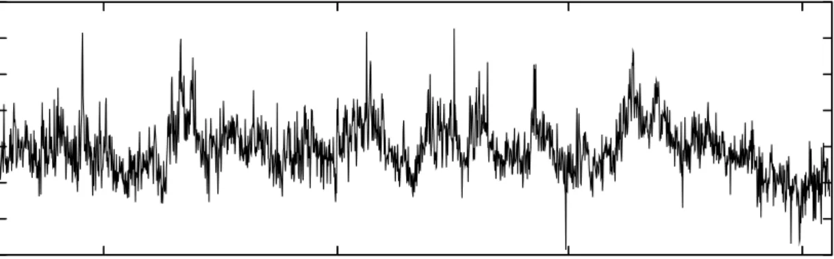
return can be treated as an unbiased estimator of the mean of latent volatility. However, it is very noisy which can be seen from its large variance. The RV row lists the statistics for the unadjusted RV. The average difference between the mean of daily squared returns and unadjusted RV is fairly large. This suggests significant market microstructure biases. The adjusted RV provides an improvement. In our work we use q= 3. The time series of adjusted log(RVt) measures are shown in Figure 1.
Market microstructure also contaminates bipower variation. As in Andersen et al. (2007) and Huang and Tauchen (2005), using staggered returns will decrease the correla-tion in adjacent returns induced by the microstructure noise. Following their suggescorrela-tion, we use an adjusted bipower variation as
[ RBPt+1 = π 2 m m−2 m ∑ j=3 |rt,j−2||rt,j|. (22) In the following we refer to adjusted RVtq as RVt, and RBP[t+1 as RBPt+1. Of course
market microstructure may also affect power variation measures, but it is much harder to correct for and empirically may be less important (Ghysels and Sinko (2006)).
5
Predictors of Realized Volatility
This section provides a brief discussion of the potential predictors that could be used to forecast realized volatility. Although daily squared returns are a natural measure of volatility, as shown by Andersen and Bollerslev (1998) they are extremely noisy. A popular proxy for volatility that exploits intraday information is the range estimator used in Brandt and Jones (2006). It is defined as ranget= log(PH,t/PL,t), where PH,t and PL,t are the intraday high and low price levels on day t. According to Alizadeh, Brandt and Diebold (2002), the log-range has an approximately Gaussian distribution, and is more efficient than daily squared returns.
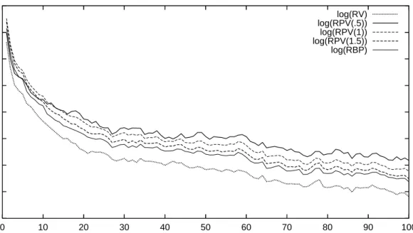
Besides lagged values of realized volatility, previous work by Forsberg and Ghysels (2007), Ghysels, Santa-Clara and Valkanov (2006) and Ghysels and Sinko (2006) has shown power variation of order 1 to be a good predictor. Other orders may be use-ful. Figure 2 displays the sample autocorrelation function for log(RVt), log(RP Vt(.5)), log(RP Vt(1)), log(RP Vt(1.5)) and log(RBPt) for the JPY-USD. The ACF for realized volatility is below all the others. Each of the power variation measures is more persistent over a wide range of lags.
Figure 3 displays estimates of corr(log(RVt),log(RP Vt−i(p))) as a function of p for different lag lengths i= 1,5,10,20. The order of RPV ranges from 0.01 to 2 with incre-ments of 0.01. Recall that RP Vt(2) = RVt. The correlation is maximized with a power variation order less than 2 in each case. The largest correlation for the JPY-USD data are: 0.6732 (i = 1, p = 1.39); 0.4906 (i = 5, p = 1.31); 0.3866 (i = 15, p = 1.25); and 0.2862 (i= 20, p= 1.01). On the other hand, the correlation with realized bipower (not shown in the figure) is always lower. For example, corr(log(RVt),log(RBPt−i)), is 0.6658 (i= 1), 0.4820 (i= 5), 0.3785 (i= 10), and 0.2745 (i= 20).
Finally, Table 2 gives out-of-sample predictive likelihoods11 and several forecast loss
functions for a linear model discussed in the next section. All models have the common regressand of log(RVt) from JPY-USD or DEM-USD but differ by the regressors. Included are versions with realized volatility, RPV(1), RPV(1.5), RBP, the daily range and daily squared returns. The range provides a considerable improvement upon daily squared re-turns, whileRV,RP V, andRBP provide further improvements. Based on the predictive likelihoods, for the JPY-USD market RP V(1) has a marginally better performance than
RV. On the other hand the version with RBP is the best in the DEM-USD market. Clearly, there is risk in selecting any one specification.
Based on this discussion we will confine model averaging to different specifications featuring realized volatility, realized power variation and realized bipower variation, and will not consider daily squared returns or the range. The specifications are discussed in the next section.
6
Models
We consider two families of linear models. The first is based on the heterogeneous au-toregressive (HAR) model of realized volatility by Corsi (2004). Corsi (2004) shows that this model can approximate many of the features of volatility including long-memory. Specifically, we use the logarithmic version (HAR-log) similar to Andersen, Bollerslev and Diebold (2007). Our benchmark model is
log(RVt,h) = β0+β1log(RVt−1,1) +β2log(RVt−5,5) +β3log(RVt−22,22)
+ βJJt−1+ut,h, ut,h vN ID(0, σ2), (23) whereRVt,h = 1h
∑h
i=1RVt+i−1 is the h-step ahead average realized volatility. This model
postulates three factors that affect volatility: a daily (h= 1), weekly (h= 5) and monthly (h= 22) factor. The importance of jumps have been recognized by Andersen, Bollerslev, and Diebold (2007), Huang and Tauchen(2005), and Tauchen and Zhou (2005) among others. All of the models include a jump term defined as
Jt = {
log (RVt−RBPt+ 1) when RVt−RBPt >0
0 otherwise (24)
where we add 1 to ensure Jt ≥ 0. For the S&P 500, an asymmetric term is included in all specifications and is defined as
Lt= {
log(RVt+ 1) when daily return<0
0 otherwise. (25)
To consider other specifications defineRP Vt,h(p) = h1 ∑h
i=1RP Vt+i−1(p) andRBPt,h = 1
h ∑h
i=1RBPt+i−1 as the corresponding average realized power and bipower variation,
re-spectively. Note the special case RVt,h =RP Vt,h(2). A summary of the specifications is
11Using the notation of Section 2.2 the predictive likelihood is computed as ∏t
j=sp(yj|Yj−1), s < t
listed in Table 3. The first panel displays HAR-type configurations. Each row indicates the regressors included in a model. A 1 indicates a daily factor (e.g. log(RP Vt−1,1(1))) a 2
means a daily and weekly factor (e.g. log(RP Vt−1,1(1)),log(RP Vt−5,5(1))) and a 3 means a
daily, weekly and monthly factor (e.g. log(RP Vt−1,1(1)),log(RP Vt−5,5(1)),log(RP Vt−22,22(1)))
using the respective regressor in that column.
Models 1–5 are HAR-log specifications in logarithms of either RV, RPV(.5), RPV(1), RPV(1.5) or RBP. Models 6–41 provide mixtures of volatility HAR terms. A typi-cal model would have regressors of log(RVt−h,h) and log (RP Vt−h,h(p)) or log(RBPt−h,h) for h = 1,5 and 22 as well as a jump term Jt−1. For instance, specification 20 has
regressors Xt−1 = [1 log(RVt−1,1) log(RVt−5,5) log(RP Vt−1,1(0.5)) log(RP Vt−5,5(0.5))
log(RP Vt−22,22(0.5)) Jt−1]. In the case of equity, Lt−1 is included, while it is omitted in
the FX applications.12
The next set of models are based on autoregressive type specifications. In the second panel of Table 3, models 42–56 are AR specifications in logarithms of either RV, RPV(.5), RPV(1), RPV(1.5) or RBP. Models 57–72 provide AR models of mixtures of volatility terms. For example, model 70 includes 10 lags of daily RV, and 5 lags of daily RPV(1), and has the form
log(RVt,h) = β0+β1log(RVt−1) +· · ·+β10log(RVt−10) +β11log(RP Vt−1(1))
+ · · ·+β15log(RP Vt−5(1)) +βJJt−1+ut,h, ut,h vN ID(0, σ2). (26) In total there are 72 different specifications that enter the model averages.
When h >1,we ensure that our predictions of log(RVt,h) are true out-of-sample fore-casts. For instance, for (23) if we used data till time t for estimation, the last regressand would be log (RVt−h+1,h), then the forecast is computed based on this information set for
E[log(RVt+1,h)|RVt, RVt−1, ...]. This is the predictive mean estimated following (3).
7
Results
We do Bayesian model comparison, and model averaging conditional on the following uniformative proper priors: β ∼ N(0,100I), and σ2 ∼ IG(0.001/2,0.001/2). For the
linear models the first 100 Gibbs draws were discarded and the next 5000 were collected for posterior inference. The output from the Gibbs sampler mixed well with a fast decaying autocorrelation function.
There areK = 72 specifications (Table 3) that enter the model averages. In performing Bayesian model averaging we follow Eklund and Karlsson (2007) and use predictive mea-sures to combine individual models. We set the model probabilities toP(Mk) = 1/K, k= 1, ..., Kat observation 500.13 Thereafter we update model probabilities according to Bayes rule. The training sample of 500 observations only affects BMA and Section 7.3 shows the results are robust to different sample sizes. The effect of the training sample is to put more weight on recent model performance. As Eklund and Karlsson (2007) show this
12Preliminary work showed no evidence of an asymmetric effect in FX data. 13For example, using (9) we setP(M
k|Y500)≡1/Kfork= 1, ..., Kand build up the model probabilities
provides protection against in-sample overfitting and can improve forecast performance. To compute the predictive likelihood from the end of the training sample to the last in-sample observation we use the Chib (1995) method14, see the Appendix for details, thereafter we update model probabilities period by period using (7) and (9).
The in-sample observations are 1000 for S&P 500, and 3000 for both JPY-USD and DEM-USD. The out-of-sample period extends from March 16, 2001 to March 30, 2004 (761 observations) for S&P 500, May 13, 1998 to December 30, 2002 (1157 observations) for JPY-USD, and May 15, 1998 to December 30, 2002 (1155 observations) for DEM-USD.
7.1
Bayesian Model Averaging
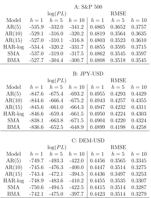
The predictive likelihood for BMA along with several benchmark alternatives is displayed in the left panel of Table 4.15 Included are autoregressive models in log(RVt), the HAR-log specification in (23), and a simple model average (SMA) which assumes equal weighting across all models through time.
Beginning with the S&P 500, BMA is very competitive. Whenh= 1, the log predictive likelihood is larger than all the benchmarks except for the AR(15) model, where BMA and AR(15) have very close values. The evidence for h = 5 and h = 10 is stronger. The log(P L) for the BMA is about 6 and 16 points larger than those from the best benchmarks. We also find the SMA is dominated by many of the benchmarks, and it has poor performance compared with BMA. The difference between these model averages is that BMA weights models based on predictive content while the SMA ignores it.
For JPY-USD market the Bayesian model average outperforms all the benchmarks for each time horizon. Compared to the HAR-log model used in Andersen, Bollerslev, and Diebold (2007) the log predictive Bayes factor in favor of BMA is 10.0, 6.9, and 12.6 for
h= 1,5, and 10, respectively. It also performs well for DEM-USD when h= 1. However for h= 5, and h= 10 the BMA is second to the AR(15) model.
In summary, in 6 out of 9 cases BMA delivers the best performance in terms of density forecasts, and when it is not the top model it is a close second.
7.2
Out-of-sample Point Forecasts
Although we focus on the predictive likelihood to measure predictive content, it is in-teresting to consider the out-of-sample point forecasts of average log volatility based on the predictive mean. Recent work by Hansen and Lunde (2006b) and Patton (2006) has emphasized the importance of using a robust criterion, such as mean squared error, to compare model forecasts against an imperfect volatility proxy like realized volatility. Therefore, the right panel of Table 4 reports the root mean squared forecast error (RMSE). The out-of-sample period corresponds exactly to the period used to calculate the predic-tive likelihood. Forecast performance is listed for the same set of models as in previous
14For instance, using the notation in Section 2, the log predictive likelihood fory
501, ..., yT, whereyT is the last in-sample observation, can be decomposed as log(p(YT))−log(p(Y500)) and each term estimated
by Chib (1995).
section.
BMA performs well against the benchmarks. For S&P 500, BMA is better than all the benchmarks for h= 5, and 10, and second best when h = 1. For JPY-USD, BMA is the top performer. As with our previous results, BMA is weaker in the DEM-USD market. In this case the SMA and the AR(15) perform well.
BMA is competitive for all data series and forecast horizons, although any improve-ments it offers are modest.16 In 5 of the 9 cases BMA has the lowest RMSE.
7.3
Training Sample
The above results are based on model combination using predictive measures. As pre-viously mentioned, we set the model probabilities to P(Mk) = 1/K, k = 1, ..., K at observation 500, thereafter model probabilities are updated according to Bayes rule. This training sample of 500 observations puts more weight on recent model performance and less on past model performance. To investigate the robustness of BMA to the size of the training sample, we calculate the results with different sample sizes as well as no training sample. Results are summarized in Table 5 for DEM-USD with similar results for the other data. Focusing on the predictive likelihood, we see that using more recent predictive measures has some benefit forh= 10.
7.4
The Role of Power Variation
In this section we investigate why BMA performs well. One reason is that it weights individual models based on past predictive content through the model probabilities. Over time model performance changes and BMA responds to it. Another possibility is that the specifications with power variation are better than existing models that only use RV.
To focus on this latter question we divide all the models that enter BMA into 3 groups according to their regressors. These are the “RV only group” which includes all models that have regressors constructed from only lag terms of log(RVt). The “RPV group” includes all models in which at least 1 RPV regressor is used, and the “RBP group” is all models that have RBP regressors. Table 6 reports the predictive likelihood of the best models within each group for each of the forecast horizonsh = 1,5, and 10. The rank of the model among the K = 72 alternatives is also displayed.
Including RPV terms can improve forecasting power. For S&P 500 when h= 1, if we exclude RPV regressors, the best individual model has a log-predictive likelihood−527.0 with a rank of 2 out of the full 72 models. Among the models with RPV, the best one has log(P L) of −526.0 and it is also the best model overall. For h = 5, including RPV
16The statistical importance of the relative RMSE values could be assessed based on a posterior
pre-dictive assessment (Gelman et al. (1996)). Using the posterior estimates for the model average based on the full set of data the steps are: 1) a draw is taken from the model probabilities; 2) given this model, a draw is taken from the respective posterior for the parameters; 3) using this parameter and model, artificial log-realized-volatility data is generated. Each of the models and the BMA is estimated and out-of-sample forecasts are produced using the generated data. This produces a RMSE for each model. Repeating this many times provides a joint distribution of RMSE’s for all models which can be used to assess the likelihood of observed results.
increases log(P L) from −310.1 for the RV group to −302.2 (rank from 13 to 1). For
h= 10, the best RPV model achieves a −299.1 with rank 1, while the best RV model is
−316.8 with rank 38.
The results from JPY-USD market provide very similar supportive evidence for the inclusion of RPV. In Panel B, the best models in the RPV group dominate those in the RV only group acrossh with much higher predictive likelihood values (−835.6 vs−844.6 for h = 1, −648.0 vs −659.4 for h = 5 and −647.9 vs −661.5 for h = 10) and ranking (1,1,1 compared with 40,22 and 22 for h= 1,5, 10). For DEM-USD data, when h= 1, the best model is from the RPV group. When h = 5 and 10, the top specification has only RV terms, however, the second best includes RPV.
In many cases models with RBP improve upon those with only RV. They increase log-predictive likelihood for S&P 500 whenh= 10, for JPY-USD across all forecast horizons, and for DEM-USD whenh= 1. However, the improvement is not as large as models with RPV terms.
In summary, as a group, specifications with RPV regressors deliver forecast improve-ments. Bipower variation delivers relatively smaller improvements over models with only realized volatility regressors. However, specifications with RPV or RBP terms also display considerable model uncertainty, but BMA gives them larger weights when they perform well.
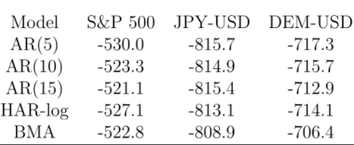
7.5
Model Risk
The message of this paper is that one should model average to reduce risk. Models that perform well in one market and forecast horizon generally do not in other cases. In fact they often perform poorly. Table 7 displays the differences in top models over markets and forecast horizons. For instance, the top JPY-USD h= 5 model, which is labeled “HAR: RV=3, PV(1)=2”, achieves log(P L) = −648.0. However, a rather different AR(15) in realized volatility is the best model in DEM-USD, h = 5. In fact, the previous model does relatively poorly with only log(P L) = −478.40, about 6 points worse than the AR(15). This example also illustrates the need to have a wide range of different model specifications, and not just the apparent top specifications that include realized power variation.
7.6
BMA with GARCH Effects
Bollerslev et al. (2007) find evidence of GARCH dynamics in time-series models of log-volatility. To investigate the importance of this for our results we consider the same set of models but include a GARCH(1,1) specification for each model. The new class of models extends those of Section 2.1 to
yt = Xt−1β+
√
htut, ut∼N(0,1) (27)
Gibbs sampling is not readily available for this model.17 Instead, we adopt the random
walk Metropolis-Hastings algorithm following Vrontos et al. (2000). The details of es-timation for this model and the predictive likelihood computation are presented in the appendix.
Table 8 compares the out-of-sample log predictive likelihood for models with GARCH errors for h = 1. All models that enter the model average have GARCH(1,1), including the benchmark specifications. Compared with Table 4, the GARCH alternatives dominate their homoskedastic counterparts. For example, the HAR-log-GARCH model improves upon the HAR-log with increases in the log(P L) of 7.3 for S&P 500, 33.5 for JPY-USD, and 34.8 for DEM-USD.
Consistent with our previous results, BMA provides overall good performance in ex-tracting predictive content from the underlying models. For JPY and DEM data, it is the top specification while it is a close second for the S&P 500. In summary, averaging over a better class of models, BMA remains a useful approach to reduce model risk and provide consistently good density forecasts.
8
Conclusion
This paper advocates a Bayesian model averaging approach to forecasting volatility. Re-cent research provides a range of potential regressors. Model averaging reduces the risk compared to selecting any one particular model. Bayesian model averaging, ranked by any of the criteria studied in this paper, is the top performer, or very close to it. This occurs over 3 different markets of realized volatility and 3 different forecast horizons. Density forecasts show the most improvement while point forecasts show only modest gains over existing benchmark models.
We find that Bayesian model averaging provides further improvements to density fore-casts when we move away from linear models and average over specifications that allow for GARCH effects. Other models that may be useful to average over include specifications with nonlinear terms and fat-tailed innovations.
9
Appendix
9.1
Marginal Likelihood
In this appendix we review the estimation of the marginal likelihood following Chib (1995). Denote the parameters θ = {β, σ2}. A rearrangement of Bayes rule gives the marginal likelihood, M L(YT), as logM L(YT) = logp ( YT|β∗, σ2∗ ) + logp(β∗, σ2∗)−logp(β∗, σ2∗|YT ) (29) wherep(YT|β∗, σ2∗) is the likelihood function, p(β∗, σ2∗) is the prior andp(β∗, σ2∗|YT) is the posterior ordinate, each evaluated atβ∗, σ2∗ which we set to the posterior mean. The
17Bauwens and Lubrano (1998) use a Griddy Gibbs sampler for GARCH models. This involves a
likelihood and prior are available and to compute the posterior ordinate note p(β∗, σ2∗|YT ) =p(β∗|YT)p ( σ2∗|YT, β∗ ) . (30)
The first term at the right hand side is,
p(β∗|YT) = ∫ p(β∗|YT, σ2 ) p(σ2|YT ) dσ2 (31)
and can be estimated as p(\β∗|YT) = N1 N ∑ i=1
p(β∗|YT, σ2(i) )
, where the draws {σ2(i)}N i=1 are
available directly from our Gibbs estimation step, and the conditional densityp(σ2∗|Y
T, β∗) is inverse-gamma as in Section 2.1 given β∗.
9.2
Estimation of Models with GARCH
We set all priors in the regression equation as before, they are independent normal
N(0,100). The GARCH parameters have independent normal N(0,100) truncated to
ω >0, a≥0, b ≥0, anda+b <1. These priors are uninformative.
Denote all the parameters by Γ ={γ1, γ2,· · · , γL}. Since the conditional distributions for some of the model parameters are unknown, Gibbs sampling is not available. Instead we use a random walk Metropolis-Hastings algorithm. If we denote all the parameters except for γl as Γ−l = {γ1,· · ·, γl−1, γl+1,· · · , γL}, we sample a new γl given Γ−l fixed. With Γ as the previous value of the chain we iterate on the following steps:
Step 1: Propose a new Γ0 according to Γ0−l = Γ−l, with element l determined as
γl0 =γl+el, el ∼N(0, ξl2). (32)
Step 2: Accept Γ0 with probability
min { p(YT|Γ 0 )p(Γ0) p(YT|Γ)p(Γ) ,1 }
and otherwise reject. p(Γ) is the prior, and
logp(YT|Γ) = T ∑ t=1 [ −1 2log(2π)− 1 2log(ht)− (yt−Xt−1β)2 2ht ] (33)
where ht = ω + a(yt − Xt−1β)2 + bht−1.18 Each ξl2 is selected to give an acceptance frequency between 0.3–0.5. Running Step 1-2 above for all the parameters l = 1,· · · , L, we obtain a new draw Γ which is one iteration. We perform 200,000 iterations and use the last 100,000 for posterior inference.
For the marginal likelihood we use the method of Gelfand and Dey (1994) adapted by Geweke (2005) (Section 8.2.4). This estimate is based onN1 ∑Ni=1g(Γ(i))/[p(YT|Γ(i))p(Γ(i))]→
p(YT)−1 asN → ∞, wherep(YT|Γ) is the likelihood, andg(Γ(i)) is a truncated multivariate Normal. Note that the prior, likelihood and g(Γ) must contain all integrating constants. Finally, to avoid underflow/overflow we use logarithms in this calculation.
18To start up the conditional variance we seth
References
[1] Alizadeh S, Brandt MW and Diebold FX. 2002. Range-Based Estimation of Stochas-tic Volatility Models. Journal of Finance 57: 1047-1091.
[2] Andersen T and Bollerslev T. 1998. Answering the Skeptics: Yes, Standard Volatility Models Do Provide Accurate Forecasts.International Economic Review 39: 885-905. [3] Andersen TG, Bollerslev T and Diebold FX. 2007. Roughing It Up: Including Jump Components in the Measurement, Modeling and Forecasting of Return Volatility.
Review of Economics and Statistics, 89, 701-720.
[4] Andersen TG, Bollerslev T, Diebold FX and Ebens H. 2001. The distribution of realized stock return volatility. Journal of Financial Economics 61: 43-76.
[5] Andersen TG, Bollerslev T, Diebold FX and Labys P. 2003. Modeling and forecasting realized volatility. Econometrica 71(2): 579-625.
[6] Andersen TG, Bollerslev T, Diebold FX and Labys P. 2001. The distribution of exchange rate volatility. Journal of the American Statistical Association 96: 42-55. [7] Andersen TG, Bollerslev T and Meddahi N. 2005. Correcting the errors: volatility
forecast evaluation using high-frequency data and realized volatilities.Econometrica
73(1): 279-296.
[8] Andreou E and Ghysels E. 2002. Rolling-sample volatility estimators: some new theoretical, simulation, and empirical results. Journal of Business and Economic Statistics 20(3): 363-76.
[9] Bandi FM and Russell JR. 2006. Separating Microstructure Noise from Volatility.
Journal of Financial Economics: forthcoming.
[10] Barndorff-Nielsen OE, Hansen P, Lunde A and Shephard N. 2006a. Designing realised kernels to measure the ex-post variation of equity prices in the presence of noise. OFRC Working Papers Series, Oxford Financial Research Centre.
[11] Barndorff-Nielsen OE, Hansen P, Lunde A and Shephard N. 2006b. Subsampling realised kernels. OFRC Working Papers Series, Oxford Financial Research Centre. [12] Barndorff-Nielsen OE and Shephard N. 2005. Variation, jumps, market frictions and
high frequency data in financial econometrics. Working paper, Nuffield College, Uni-versity of Oxford.
[13] Barndorff-Nielsen OE and Shephard N. 2004. Power and bipower variation with stochastic volatility and jumps.Journal of Financial Econometrics 2(1): 1-37. [14] Barndorff-Nielsen OE and Shephard N. 2002a. Econometric analysis of realized
volatility and its use in estimating stochastic volatility models.Journal of the Royal Statistical Society, Series B, 64: 253-280.
[15] Barndorff-Nielsen OE and Shephard N. 2002b. Estimating quadratic variation using realised variance. Journal of Applied Econometrics 17: 457-477.
[16] Bauwens L. and Lubrano M. 1998 Bayesian Inference on GARCH Models Using the Gibbs Sampler. The Econometrics Journal 1(1): 23-46.
[17] Bollerslev T, Kretschmer U, Pigorsch C and Tauchen G. 2007. A Discrete-Time Model for Daily S&P 500 Returns and Realized Variations: Jumps and Leverage Effects. forthcoming Journal of Econometrics.
[18] Bollerslev T and Zhou H. 2002. Estimating stochastic volatility diffusion using con-ditional moments of integrated volatility. Journal of Econometrics 109(1): 33-65. [19] Box GEP. 1980. Sampling and Bayes’ inference in scientific modelling and robustness.
Journal of the Royal Statistical Society A, 143: 383-430.
[20] Brandt MW and Jones CS. 2006. Volatility Forecasting with Range-Based EGARCH Models.Journal of Business and Economic Statistics 24: 470-486.
[21] Chib S. 1995. Marginal likelihood from the Gibbs output. Journal of the American Statistical Association 90(432): 1313–1321.
[22] Chib S. 2001. Markov Chain Monte Carlo Methods: Computation and Inference. In Handbook of Econometrics: volume 5, Heckman JJ and Leamer E, eds. North Holland, Amsterdam, 3569-3649.
[23] Corsi F. 2004. A simple long memory model of realized volatility. Working paper, University of Southern Switzerland.
[24] Ding Z, Granger CWJ and Engle RF. 1993. A long memory property of stock market returns and a new model.Journal of Empirical Finance 1: 83-106.
[25] Eklund J and Karlsson S. 2007. Forecast Combination and Model Averaging Using Predictive Measures. Econometric Reviews 26(2-4): 329 - 363.
[26] Fernandez C, Ley E and Steel MJF. 2001. Model Uncertainty in Cross-Country Growth Regressions. Journal of Applied Econometrics 16(5): 563-576.
[27] Fleming J, Kirby C and Ostdiek B. 2003. The economic value of volatility timing using ’realized’ volatility.Journal of Financial Economics 67: 473-509.
[28] Forsberg L and Ghysels E. 2007. Why Do Absolute Returns Predict Volatility So Well? Journal of Financial Econometrics 5: 31-67.
[29] French K, Schwert GW and Stambaugh RF. 1987. Expected Stock Returns and Volatility.Journal of Financial Economics 19: 3-29.
[30] Gelfand AE and Dey D. 1994. Bayesian model choice: asymptotic and exact calcu-lations.Journal Royal Statistical Society B, 56: 501-514.
[31] Gelman A, Meng X and Stern H. 1996. Posterior Predictive Assessment of Model Fitness via Realized Discrepancies. Statistica Sinica. 6(4) 733-807.
[32] Geweke J. 2005.Contemporary Bayesian Econometrics and Statistics. John Wiley & Sons Ltd.
[33] Geweke J. 1995. Bayesian comparison of Econometric Models. Working paper, Re-search Department, Federal Reserve Bank of Minneapolis.
[34] Geweke J and Whiteman C. 2005. Bayesian Forecasting. Forthcoming in Handbook of Economic Forecasting, Graham E, Granger C and Timmermann A, eds. Elsevier. [35] Ghysels E, Santa-Clara P and Valkanov R. 2006. Predicting volatility: How to get most out of returns data sampled at different frequencies. Journal of Econometrics,
131: 59-95.
[36] Ghysels E and Sinko A. 2006. Comment on Hansen and Lunde JBES paper.Journal of Business and Economic Statistics 24(2): 192-194.
[37] Ghysels E, Sinko A and Valkanov R. 2007. MIDAS Regressions: Further Results and New Directions. Econometric Reviews 26(1): 53 - 90.
[38] Gordon S. 1997. Stochastic trends, deterministic trends, and business cycle turning points.Journal of Applied Econometrics 12: 411-434.
[39] Hansen PR and Lunde A. 2006a. Realized Variance and Market Microstructure Noise.
Journal of Business and Economic Statistics 24(2) 127-161.
[40] Hansen, PR and Lunde A. 2006b. Consistent ranking of volatility models.Journal of Econometrics 131: 97-121.
[41] Hibon M and Evgeniou T. 2004. To combine or not combine: selecting among fore-casts and their combinations. International Journal of Forecasting 21(1): 15-24. [42] Hoeting JA, Madigan D, Raftery A and Volinsky CT. 1999. Bayesian Model
Aver-aging: A Tutorial.Statistical Science 14(4): 382-417.
[43] Hsieh D. 1991. Chaos and Nonlinear Dyanmics: Application to Financial Markets.
Journal of Finance 46: 1839-1877.
[44] Huang X and Tauchen G. 2005. The Relative Contribution of Jumps to Total Price Variance. Journal of Financial Econometrics 3: 456-499.
[45] Jacobson T and Karlsson S. 2004. Finding good predictors for Inflation: A Bayesian Model Averaging Approach. forthcoming, Journal of Forecasting.
[46] Kass RE and Raftery AE. 1995. Bayes factors and model uncertainty.Journal of the American Statistical Association 90: 773-795.
[47] Koop G. 2003.Bayesian Econometrics. John Wiley & Sons Ltd.
[48] Koop G and Potter S. 1999. Bayes factors and nonlinearity: Evidence from economic time series. Journal of Econometrics 88: 251-282.
[49] Koop G and Potter S. 2004. Forecasting in dynamic factor models using Bayesian model averaging.The Econometrics Journal 7(2): 550-565.
[50] Koopman SJ, Jungbacker B and Hol E. 2005. Forecasting daily variability of the S&P 100 stock index using historical, realised and implied volatility measurements.
Journal of Empirical Finance 12(3): 445-475.
[51] Liu C and Maheu J. 2008. Are there structural break in Realized Volatility? forth-coming Journal of Financial Econometrics.
[52] Maheu J and McCurdy TH 2002. Nonlinear Features of Realized FX Volatility. Re-view of Economics and Statistics 84(4): 668-681.
[53] Martens M and van Dijk D.J.C. and de Pooter M. 2004. Modeling and forecasting S&P 500 volatility: Long memory, structural breaks and nonlinearity. Discussion Paper, Tinbergen Institute.
[54] Meddahi N. 2002. A Theoretical Comparison Between Integrated and Realized Volatility.Journal of Applied Econometrics 17: 479-508.
[55] Meddahi N. 2003. ARMA Representation of Integrated and Realized Variances.The Econometrics Journal 6: 334-355.
[56] Min C and Zellner A. 1993. Bayesian and non-Bayesian methods for combining mod-els and forecasts with applications to forecasting international growth rates. Journal of Econometrics 56(1-2): 89-118.
[57] Oomen RCA. 2005. Properties of bias-corrected realized variance under alternative sampling schemes. Journal of Financial Econometrics 3(4): 555-577.
[58] Patton A. 2006. Volatility Forecast Comparison using Imperfect Volatility Proxies. Working paper 175, Quantitative Finance Research Centre, University of Technology Sydney.
[59] Pesaran MH and Zaffaroni P. 2005. Model Averaging and Value-at-Risk Based Evalu-ation of Large Multi-Asset Volatility Models for Risk Management. CEPR Discussion Papers 5279.
[60] Raftery A.E. and Madigan D. and Hoeting J.A. 1997. Bayesian Model Averaging for Linear Regression Models. Journal of the American Statistical Association 92(437) 179-191.
[61] Schwert GW. 1989. Why Does Stock Market Volatility Change Over Time? Journal of Finance 44: 1115-1154.
[62] Tauchen G and Zhou H. 2005. Identifying Realized Jumps on Financial Markets. Working Paper, Duke University.
[63] Vrontos I. D. and Dellaportas P. and Politis D. N. 2000. Full Bayesian Inference for GARCH and EGARCH Models.Journal of Business and Economics Statistics 18(2), 187-198.
[64] Wright JH. 2003. Forecasting U.S. inflation by Bayesian Model Averaging. Interna-tional Finance Discussion Paper, The Federal Reserve Board.
[65] Zhang L and Mykland P and Ait-Sahalia Y. 2005. A tale of two time scales: de-termining integrated volatility with noisy high-frequency data.Journal of American Statistical Association 100(472), 1394-1411.
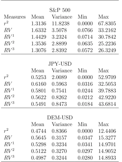
Table 1: Summary Statistics for Measures of Volatility
S&P 500
Measures Mean Variance Min Max
r2 1.3136 11.8238 0.0000 67.8305 RV 1.6332 3.5078 0.0766 33.2162 RV1 1.4429 3.2324 0.0714 30.7842 RV2 1.3536 2.8899 0.0635 25.2236 RV3 1.3076 2.8392 0.0572 26.3249 JPY-USD
Mean Variance Min Max
r2 0.5253 2.0089 0.0000 52.9709 RV 0.6160 0.5963 0.0316 32.5053 RV1 0.5801 0.7541 0.0244 39.7883 RV2 0.5622 0.8262 0.0212 42.9220 RV3 0.5491 0.8473 0.0184 43.6814 DEM-USD
Mean Variance Min Max
r2 0.4744 0.8366 0.0000 12.4406
RV 0.5645 0.3157 0.0347 15.3277
RV1 0.5298 0.3234 0.0341 14.9701
RV2 0.5122 0.3270 0.0297 14.9052
RV3 0.4987 0.3244 0.0280 14.8933
S&P 500 data is from February 6, 1997 to March 30, 2004 (1796 observations). JPY-USD data, February 3, 1986 to December 30, 2002 (4192 observations). DEM-USD data, February 3, 1986 to December 30, 2002 (4190 observations). r2 is the daily squared return, RV is unadjusted realized volatility,RV1,RV2
Table 2: Model Comparison Using Different Volatility Predictors for FX Volatility
JPY-USD
Regressors
RV RP V(1) RBP Range Squared Return
log(P L) -845.32 -845.12 -856.87 -863.47 -997.31 RMSE 0.4918 0.4864 0.4949 0.5025 0.5620 MAE 0.3659 0.3601 0.3684 0.3851 0.4285 R2 0.5419 0.5594 0.5498 0.5193 0.4141 DEM-USD Regressors
RV RP V(1.5) RBP Range Squared Return
log(P L) -754.71 -752.04 -748.06 -765.03 -872.84 RMSE 0.4467 0.4450 0.4437 0.4521 0.4937
MAE 0.3346 0.3374 0.3311 0.3889 0.3729
R2 0.3954 0.3988 0.3997 0.3996 0.3085 This table compares the out-of-sample forecasting power of different regressors using JPY-USD and DEM-USD data. The out-of-sample period is May 13, 1998 to December 30, 2002 (1157 observations) for JPY-USD, and May 15, 1998 to December 30, 2002 (1155 observations) for DEM-USD. The common model is a HAR-log
log(RVt) =β0+β1log(Vt−1,1)+β2log(Vt−5,5)+β3log(Vt−22,22)+ut, ut∼N(0, σ2), where Vt,h = h1
∑h
i=1Wt+i−1. For the JPY-USD column 2 sets Wt−1 = RVt−1,
column 3 Wt−1 = RP Vt−1(1), column 4 Wt−1 = RBPt−1, column 5 Wt−1 =
ranget−1 = log(PH,t−1/PL,t−1), and column 6 Wt−1 = rt2−1, the daily squared
return. It is identical for the DEM-USD except that column 3 sets Wt−1 =
RP Vt−1(1.5). PH,t−1 and PL,t−1 are the intraday high and low price levels on
day t−1. For the out-of-sample period we report the log predictive likelihood (PL), root mean square error (RMSE) and mean absolute error (MAE) for the predictive mean, and the R2 from a forecast regression of realized volatility on a
Table 3: Model Specifications HAR-type AR-type Model RV RPV(.5) RPV(1) RPV(1.5) RBP Model RV RPV(.5) RPV(1) RPV(1.5) RBP 1 3 0 0 0 0 42 5 0 0 0 0 2 0 3 0 0 0 43 0 5 0 0 0 3 0 0 3 0 0 44 0 0 5 0 0 4 0 0 0 3 0 45 0 0 0 5 0 5 0 0 0 0 3 46 0 0 0 0 5 6 1 1 0 0 0 47 10 0 0 0 0 7 1 2 0 0 0 48 0 10 0 0 0 8 1 3 0 0 0 49 0 0 10 0 0 9 1 0 1 0 0 50 0 0 0 10 0 10 1 0 2 0 0 51 0 0 0 0 10 11 1 0 3 0 0 52 15 0 0 0 0 12 1 0 0 1 0 53 0 15 0 0 0 13 1 0 0 2 0 54 0 0 15 0 0 14 1 0 0 3 0 55 0 0 0 15 0 15 1 0 0 0 1 56 0 0 0 0 15 16 1 0 0 0 2 57 5 1 0 0 0 17 1 0 0 0 3 58 5 0 1 0 0 18 2 1 0 0 0 59 5 0 0 1 0 19 2 2 0 0 0 60 5 0 0 0 1 20 2 3 0 0 0 61 5 5 0 0 0 21 2 0 1 0 0 62 5 0 5 0 0 22 2 0 2 0 0 63 5 0 0 5 0 23 2 0 3 0 0 64 5 0 0 0 5 24 2 0 0 1 0 65 10 1 0 0 0 25 2 0 0 2 0 66 10 0 1 0 0 26 2 0 0 3 0 67 10 0 0 1 0 27 2 0 0 0 1 68 10 0 0 0 1 28 2 0 0 0 2 69 10 5 0 0 0 29 2 0 0 0 3 70 10 0 5 0 0 30 3 1 0 0 0 71 10 0 0 5 0 31 3 2 0 0 0 72 10 0 0 0 5 32 3 3 0 0 0 33 3 0 1 0 0 34 3 0 2 0 0 35 3 0 3 0 0 36 3 0 0 1 0 37 3 0 0 2 0 38 3 0 0 3 0 39 3 0 0 0 1 40 3 0 0 0 2 41 3 0 0 0 3
The first panel displays HAR-type model configurations. A 1 indicates a daily factor (e.g. log(RP Vt−1,1(1))) a
2 means a daily and weekly factor (e.g. log(RP Vt−1,1(1)),log(RP Vt−5,5(1))) and a 3 means a daily, weekly and
Table 4: Out-of-Sample Forecasts, log(RVt,h) A: S&P 500 log(P L) RMSE Model h= 1 h= 5 h = 10 h= 1 h= 5 h= 10 AR(5) -535.9 -332.0 -341.2 0.4865 0.3652 0.3757 AR(10) -529.1 -316.0 -320.2 0.4819 0.3564 0.3635 AR(15) -527.0 -310.1 -316.8 0.4803 0.3523 0.3610 HAR-log -534.4 -320.2 -331.7 0.4855 0.3595 0.3715 SMA -537.0 -319.0 -317.5 0.4862 0.3545 0.3597 BMA -527.7 -304.4 -300.7 0.4808 0.3518 0.3545 B: JPY-USD log(P L) RMSE Model h= 1 h= 5 h = 10 h= 1 h= 5 h= 10 AR(5) -847.6 -675.4 -693.2 0.4955 0.4293 0.4429 AR(10) -844.6 -666.4 -675.2 0.4943 0.4257 0.4355 AR(15) -845.6 -661.0 -664.3 0.4947 0.4232 0.4311 HAR-log -846.6 -659.4 -661.5 0.4950 0.4224 0.4303 SMA -838.1 -663.8 -671.5 0.4904 0.4220 0.4324 BMA -836.6 -652.5 -648.9 0.4899 0.4198 0.4258 C: DEM-USD log(P L) RMSE Model h= 1 h= 5 h = 10 h= 1 h= 5 h= 10 AR(5) -749.7 -493.3 -422.0 0.4456 0.3565 0.3345 AR(10) -745.6 -476.3 -400.0 0.4447 0.3514 0.3275 AR(15) -743.4 -472.1 -394.5 0.4436 0.3497 0.3253 HAR-log -748.9 -483.6 -410.2 0.4455 0.3535 0.3307 SMA -750.6 -494.5 -422.5 0.4415 0.3514 0.3287 BMA -742.1 -475.0 -397.7 0.4423 0.3514 0.3279
This table reports the out-of-sample log predictive likelihood (log(P L)), and the out-of-sample root mean square forecast error (RMSE) for the predictive mean. The results are for Bayesian Model Averag