Clemson University
TigerPrints
All Dissertations Dissertations
5-2012
Hedonic Prediction and Likeability Effects in
Evaluating Biodata for Selection
Peggy Tyler
Clemson University, [email protected]
Follow this and additional works at:https://tigerprints.clemson.edu/all_dissertations Part of thePsychology Commons
This Dissertation is brought to you for free and open access by the Dissertations at TigerPrints. It has been accepted for inclusion in All Dissertations by an authorized administrator of TigerPrints. For more information, please [email protected].
Recommended Citation
Tyler, Peggy, "Hedonic Prediction and Likeability Effects in Evaluating Biodata for Selection" (2012).All Dissertations. 898. https://tigerprints.clemson.edu/all_dissertations/898
HEDONIC PREDICTION AND LIKEABILITY EFFECTS IN EVALUATING BIODATA FOR SELECTION
A Thesis Presented to the Graduate School of
Clemson University
In Partial Fulfillment
of the Requirements for the Degree Doctor of Philosophy Industrial/Organizational Psychology by Peggy Tyler May 2012 Accepted by:
Dr. Fred Switzer, Committee Chair Dr. Cynthia Pury
Dr. Deborah Switzer Dr. Johnell Brooks
ABSTRACT
Employees involved in the selection process for new co-workers are conventionally thought to be acting as agents for the interests of the hiring
organization. But do individuals act as effective surrogates or are they making emotional predictions about their own personal compatibility with a potential colleague that
influence their subsequent judgments? Three interlinking studies examined this question. First, a meta-analysis of the relationship between likeability and hireability was
conducted in order to determine the effect size for the relationship between likeability and hiring. A corrected effect size of .60 indicated that likeability was a substantial factor in hiring, but there was a very large percentage of uncorrected variance indicating the presences of an unknown moderator or moderators. It was speculated that that the most likely moderator is selector experience.
The second study examined if likeability is a factor in hiring even when it is not a factor in job performance (i.e., when likeability is irrelevant to or independent of job performance). In this online decision study an eportfolio for a highly-qualified, yet unlikeable, candidate was presented to 112 university faculty, who were asked to rate the candidate’s hireability/potential job performance. The participants were each told that the candidate was either a new colleague or was working in another department, testing the hypothesis that this unlikeable but capable applicant’s expected job performance would be rated higher if he was not working with the assessor. This hypothesis was not supported; the faculty did not significantly hire based on their hedonic predictions.
Finally, a utility analysis was performed in order to gauge the practical cost of an organization preferentially hiring more civil/collegial employees. A Monte Carlo
simulation was conducted to assess the potential financial impact of replacing top “uncivil” candidates with lower-ranking collegial ones. Taken together, these studies provide for a more accurate picture of individual behavior and judgment in real-world selection and form a basis for further exploration into institutional and personal trade-offs between employee competence and collegiality.
ACKNOWLEDGEMENTS
I would like to thank my advisor, Fred Switzer, for his patience, endurance, and good humor during this incredibly long and tortuous process. I would also like to thank my other committee members, Cindy Pury, Debi Switzer, and Johnell Brooks, for their persistent support and optimism. I also very much appreciate the help of Rich Pak for his advice and coding efforts.
Finally, I would like to thank Pat Raymark for his encouragement and generosity in seeing me through to the end of this protracted endeavor – his help made it possible to finally complete it.
TABLE OF CONTENTS
Page
TITLE PAGE ... i
ABSTRACT ... ii
ACKNOWLEDGEMENTS ... iv
LIST OF TABLES ... vii
LIST OF FIGURES ... viii
CHAPTERS I. INTRODUCTION ... 1
Hedonic Prediction... 1
Hedonic Prediction and Motivation ... 6
Hedonic Prediction in the Workplace ... 7
Employee Selection as Hedonic Prediction ... 8
Biodata and Selection ... 9
Likeability and Selection ... 10
Likeability and Competence ... 14
II. METHOD ... 16
Procedure ... 16
Study 1: Meta-Analysis... 16
Study 2: Decision Study... 18
Study 2a: Undergraduate Sample... 23
Study 3: Utility Analysis ... 24
III. RESULTS ... 29
Study 1: Meta-Analysis... 29
Study 2: Decision Study... 33
Other Survey Respondents ... 39
Table of Contents (Continued) Page IV. DISCUSSION ... 43 Limitations ... 48 Future Research ... 49 Conclusions ... 50 APPENDICES ... 52
A: Studies Rejected from Meta-Analysis ... 53
B: Studies Rejected from Meta-Analysis: References... 55
C: Studies Included in Meta-Analysis ... 59
D: Meta-Analysis Coding Sheet ... 62
E: Recruitment Email ... 63
F: Participation Agreement ... 64
G: Emails to Participants (with Survey Links) ... 66
H: Position Description ... 68
I: Candidate Resume ... 69
J: Letters of Recommendation ... 70
K: Survey ... 73
L: Position Description with Undergraduate Responsibilities ... 81
M: Meta-Analysis Studies: Coded Data ... 82
N: Decision Study Descriptive Statistics ... 85
O: Decision Study Correlation Matrix ... 88
P: Emotion Word Frequencies from Faculty Comments ... 89
Q: Job Performance Word Frequencies from Faculty Comments ... 91
LIST OF TABLES
Table Page
3.1 Meta-analysis of correlations between likeability
and hireability………29 3.2 Meta-analysis of correlations between likeability
and hireability (no outliers)………31 3.3 t-test of hiring recommendations in the “working with”
and “not working with” condition………..34 3.4 t-test of hedonic predictions for self and others in the
“working with” and “not working with” conditions………..35 3.5 Total of faculty participants who disagree with hiring
candidate across “working with” and “not working
with” conditions……….36 3.6 t-tests of hiring and interview recommendations in the
“working with” and “not working with” conditions………..40 3.7 t-test of hiring recommendations in the “working with”
and “not working with” conditions (Undergraduates)………...41 3.8 Results of utility analysis: cost of civility………....42
LIST OF FIGURES
Figure Page
3.1 Graph of meta-analysis effect size estimates……….30 3.2 Word cloud of comments from faculty participants who
disagree with hiring candidate across “working with”
and “not working with” conditions (the 24% group)……….…………..38 3.3 Word cloud of comments from faculty participants who
were neutral or agreed or strongly agreed that the candidate should be hired (across “working with” and “not working
CHAPTER ONE INTRODUCTION
It is generally assumed that individuals who screen and select job applicants for positions act as agents for their organizations’ interests. In the cases where human
resource professionals select employees for departments with which they seldom interact, or managers hire for levels several layers below them, this seems like a reasonable
assumption, but what about situations in which employees are involved in choosing their future co-workers?
Faculty search committees, engineering workteams, law firms, and other professional occupations are often in the position of screening and selecting potential colleagues. Is there more than organizational surrogacy involved in the decision-making process of an employee selecting someone that he or she will be interacting with on a regular basis? It seems very likely that, in these cases, selectors make hedonic predictions about how much they will enjoy working side by side with candidates – predictions that would certainly influence their hiring decisions.
Hedonic Prediction
The first researcher to describe the process of making judgments about future emotions as hedonic prediction was Nobel-Prize-winning psychologist Daniel Kahneman in an experiment at Stanford with his student Jackie Snell. They constructed a series of hypotheses testing the ability of people to predict their own future likes and dislikes and to make optimal choices and decisions based on these projections of their prospective affect (Kahneman & Snell, 1990; Snell, 1991). In their classic study of the accuracy of
hedonic predictions (Kahneman & Snell, 1992), college students ate ice cream or yogurt while listening to music, and rated their enjoyment on a -6 to +6 scale. After the
participants predicted how much they would like to repeat this experience every day for a week, repeated the daily experience, and then rated it again, Kahneman and Snell found that there was little or no correlation between their actual and predicted liking. This experiment was repeated (this time using unfamiliar snack foods and body care products) by Rozin, Hanko and Durlach (2006), who compared student-parent pairs to see if a “generation of experience” would improve the ability to predict. Once again, predictions were compared to actual liking after a week, and parents were no better than students at projecting their “hedonic trajectories.”
Other researchers have used the label affective forecasting for this estimation of emotional response to future events. Credit for earliest citation goes to Harvard’s Daniel Gilbert (Gilbert, Pinel, Wilson, Blumberg & Wheatley, 1998) but Totterdell (Totterdell, Parkinson, Briner, & Reynolds, 1997) also was talking about “forecast” of affect around the same time. As the East and West coast contingents weighed in for domination of the terminology describing the concept, researchers agreed on the basic fact that people could be counted on to mispredict how much pleasure or displeasure future scenarios would bring – the sources of the cognitive error were the real focus of their interest.
Wilson & Gilbert (2003) state, “Affective forecasts can be broken down into four components: predictions about the valence of one’s future feelings, the specific emotions that will be experienced, the intensity of the emotions, and their duration.” These four components also are the sources of much of the predictive error.
Valence, the positive or negative direction of the future affective state, can usually be quite accurately predicted by a person with experience in that domain. If asked if having lemon juice squirted in your eye tomorrow will be a positive or negative event you will probably forecast accurately. If told you would receive a $10 Starbucks coupon at your next visit, you would most likely be happy if a Starbucks was conveniently located and you liked their menu. In a simulated dating game experiment (Wilson, Wheatley, Kurtz, Dunn, & Gilbert, 2004), students competed for a hypothetical date and were randomly assigned to win or lose. All of the participants predicted that they would be in a better mood if they won than if they lost, and all of the winners did report better moods than the losers. In their experiment described earlier, Kahneman and Snell (1992), did have participants who made valence errors – they found that some students began to like plain yogurt more than they thought they would after an initial first taste, and others discovered that a full serving was not as pleasant to eat as a sample was. There were also valence errors made by some participants in mistaken predicting that daily repetition would decrease their liking of music or of ice cream. In Rozin, Hanko and Durlach’s (2006) study, the percentage of participants who correctly predicted their direction of change in liking was less than 64% for any of the four items. (Mispredictions in valence went in both directions, so “mere exposure” effect (Zajonc, 1968) – increasing liking of the unfamiliar – was not the explanation here or in the Kahneman and Snell experiment.)
A simple change in affective direction needs to be labeled with a specific emotion to have meaning. The lemon juice in the eye should bring about a negative change in affect – but will it be rage or sorrow or fear or confusion or disgust or none or all or some
of the above? People are generally accurate in predicting discrete emotions. For
example, Robinson and Clore (2001) gave participants written descriptions of a series of pictures that were chosen to trigger specific emotions (fear, disgust, etc.) and asked them to predict on how each picture would make them feel; their predictions closely matched the responses of participants who were shown the pictures. However, the future seldom presents situations requiring such a simple emotional response – mixed feelings are usually the rule, even if people tend to discount this emotional complexity in their
forecasts. College students asked to imagine their graduation day projected joy and pride but overlooked sadness and apprehension (Larsen, McGraw & Cacioppo, 2001).
Liberman, Sagristano, and Trope (2002) found that people predicted more accurately mixed emotions for near-future events, but used more basic (and inaccurate) forecasts of affect for far-future events.
When Woodzicka and Lafrance (2001) asked women to imagine scenarios of being sexually harassed, the women responded that they would feel angry and
confrontative, not predicting the more complex mixed feelings of fear and concern for jeopardizing their employment.
Another mistake that people make in predicting their future emotions is overestimating the intensity of their reactions to situation or event. This bias was best shown in a study where students were asked to predict how they would feel the moment they learned their final grade in their psychology class, on Christmas day, and other events in their lives(Buehler & McFarland, 2001). Students projected that they would feel more intense emotions than they actually experienced when they focused on these
events discretely, but when experimenters asked them to consider a set of relevant past experiences before predicting future affect levels, the intensity bias was dampened.
A study of the ability of people to accurately predict the duration of their emotional reactions (Gilbert, Pinel, Wilson, Blumberg, & Wheatley, 1998) required participants to estimate their projected affect at future points in time for scenarios such as after the breakup of a romantic relationship, achieving tenure (or not), the defeat or election of a preferred candidate, or negative personality feedback. Participants overpredicted the length the time these events would have an emotional effect for both positive and negative reactions. Gilbert et al. blamed this durability bias on immune neglect – a failure to recognize that not only do feelings fade over time as a matter of course, but the mental-health-protecting “psychological immune system” muffles them. Durability bias is also blamed on focalism (Wilson, Wheatley, Meyers, Gilbert, & Axsom, 2000), where people focus too much on one specific future occurrence and not enough on the outcomes of the other events that surround it – college football fans were less likely to overpredict how long the outcome of a game would influence their
happiness if they first thought about how much time they would spend on other future activities.
In researching how people make hedonic predictions (and therefore errors), differentiating duration from intensity is not necessarily possible. These two components of error in affective forecasting are now usually referred to together as impact bias (Gilbert, Driver-Linn, & Wilson, 2002). More recent research in Gilbert and Wilson’s lab (Morewedge, Gilbert, & Wilson, 2005) resulted in the conclusion that “impact bias
may be due in part to people's reliance on highly available but unrepresentative
memories.” The idea that people select atypical exemplars from their pasts for clues to future affect is another link back to the original work of Kahneman (1994), who also suggested that error in making “rational” decisions in the affective domain can be the result of confabulated memory and incorrect evaluation of past experience.
Another source of error beyond Wilson and Gilbert’s (2003) model is distinction bias (Hsee & Zhang, 2004). It can be a source of error when a person is confronted with evaluation of multiple options or scenarios. In the Hsee & Zhang study, people predicted how much they would like or dislike reading different-length lists of positive and
negative words or recalling good or bad stories about themselves while eating chocolate – they overpredicted a wider range of affective impacts for choices when in “joint
evaluation” mode than when evaluating items individually.
So knowing that we make hedonic predictions often and in many domains, yet are prone to many types of errors, lets us look at a wide range of behaviors and actions for the possible effect of either mispredictions or not taking hedonic predictions into consideration.
Hedonic Prediction and Motivation
Hedonic prediction is a crucial component of motivation. When you made the choice to read this document, you made a hedonic prediction – you projected future emotions you thought you would have after reading this dissertation. And, according to Vroom’s (1964) Valence-Instrumentality-Expectancy (VIE) model of motivation, this prediction helped you choose among the other tasks competing for your attention – that
rerun of “America’s Next Top Model,” your messy sock drawer, your own research. Boiled down to the simplest version of VIE, you compared your hedonic prediction to the positivity or negativity of completing other possible tasks and picked this task as the most positive (or least aversive).
Very little research seems to be explicitly examining the role of hedonic
prediction in motivation. Sheldon, Gunz, Nichols, & Ferguson (2010), looked at hedonic prediction and extrinsic and intrinsic goal-setting. They found that hedonic
overestimation may account for some of the allure of extrinsic goals, even though their research showed that intrinsic goal attainments resulted in more happiness. Maclnnis and Patrick (2006) examined goals from a different angle in their model of consumer impulse control, with hedonic prediction as the determining factor among competing motivational conflicts (i.e., approach-avoidance).
Hedonic Prediction in the Workplace
A comprehensive literature review also resulted in almost no relevant research of hedonic prediction in work settings. Gilbert, Pinel, Wilson, Blumberg, & Wheatley (2002) used work situations to study durability bias: they looked at the affective forecasts of University of Texas faculty considered for tenure, and conducted an experiment hiring undergraduates as hypothetical product testers in fair and unfair conditions to test the duration of the applicants’ affective reaction to the selection process.
In 2003, Richard Coughlin asked hotel managers to predict numerical outcomes important to their jobs (occupancy, turnover, revenue) and how satisfied they would be
with outcomes at various ranges around their predicted values. Managers tended to overestimate the impact that unexpectedly high or low outcomes would have on their satisfaction levels.
A noteworthy review article appeared in the Indiana Law Journal in 2005. Jeremy Blumenthal earned a psychology Ph.D. under Daniel Gilbert at Harvard and followed it with a law degree. His “Law and the Emotions: The Problems of Affective Forecasting” addresses how affective misprediction affects criminal and civil trials, contract law, capital punishment statutes, and health and employment policies. Blumenthal states that jurors’ overestimates of the intensity and duration of future pain and suffering in civil damage cases results in overcompensation or tort victims; likewise victims’ impact statements in death penalty cases may cause jurors to overestimate the future effect of the defendants’ crimes on victims. His novel suggestion is to put affective forecasting experts on the stand to admit evidence on predicting future emotion to juries in such cases.
Given the impact of hedonic prediction on motivation, this is a seriously neglected opportunity for researchers to look at individuals’ emotional forecasts in the workplace.
Employee Selection as Hedonic Prediction
Selection is a workplace prediction made by individuals on behalf of the
organization. Employee selection is partly a social process, but social process research in employee selection has gone only as far as looking at “identity” – the roles that
employee selection different from previous work looking at other similar selection bias? Because this is a hedonic prediction about the selector himself/herself – not the company or the environment or the culture or the position. The hedonic prediction makes the following question into a predictor (weight unknown) in the selection process: How will I feel sitting next to this person in meetings? Hedonic prediction potentially puts the selector in a dilemma – the organization’s goals versus the selector’s goals.
Biodata and Selection
Selectors use many sources of information about candidates to make their
decisions; in the screening phase, what is most typically available to them is “biodata” – biographical data. This could be an application form or a letter of intent or a résumé. In some cases, applicants are asked to include letters of reference with their résumés, which are also rich sources of biodata, with the bonus of being from second-hand, ostensibly-objective observers.
Biodata has been criticized, with detractors citing applicant faking and
inconsistent and unsystematic use by employers (Breaugh, 2009), but this same author notes that criticism is outweighed by “substantial evidence documenting its value as a predictor” (p. 219).
A study by Nicklin and Roch (2009) reported that the academics that they
surveyed placed more weight on letters of recommendation than applied professionals did for selection decisions. The applied professionals in their sample were also actually willing to stop using letters of reference entirely as selection tools and agreed with a
statement that research on letters of reference in selection should be discontinued. The academic sample did not agree with either of those items.
Colarelli, Hechanova-Alampay, and Canali (2002) speculate that letters of recommendation appeal to selectors because of humans’ evolutionary preference for narrative information about people. Going back to motivational theory, they also posit that these letters are important sources for loss-aversion decision making (Kahneman & Tversky, 1979) – “losses loom larger than gains” – and if negative information is
available about a candidate that will let the selector avoid “harm,” that is where it will be reside. They note that despite knowledge of letters of recommendations’ weaknesses among industrial/organization psychology and human resource management faculty, most advertisements for teaching and graduate positions in require them, implying a basic human attachment if not an evolutionary mechanism.
Likeability and Selection
Making a hedonic prediction about your own future emotions can certainly be linked to feelings of like or dislike about a prospective colleague. But even though we can probably describe liking when we see it, likeability is a noteworthy construct to define from a research standpoint.
The original citation for most industrial/organizational (I/O) psychology
researchers who discuss likeability is Keenan (1977), who asked103 graduate recruitment interviewers to interview 187 students at Heriot-Watt University and give a general evaluation of each of them, along with ratings of each candidate’s chances of obtaining a follow-up interview or a job offer with their company. The interviewers also rated each
student on intelligence, morality, and a six-point scale for how much they would
“probably like this person” and how much they would “enjoy working with this person” (from Byrne’s (1971) Interpersonal Judgment Scale – these two items have a correlation of 0.78). He found a strong relationship between liking and general ratings, a
relationship that was much higher among the 13% of the interviewers who expected to work with the candidates personally than those who did not – 0.75 versus 0.43.
Keenan uses the phrase “personal attraction” as a synonym for “liking” in his article, which at first is jarring, because that seems to imply a sexual or romantic or amatory component that isn’t part of the construct. However, it seems that this was fairly common in the 1970s – when Helmreich, Aronson and LeFan (1970) famously had competent and incompetent job applicants spill coffee on themselves (and the competent spillers became far more likeable), they labeled their research as a study of “a pratfall on interpersonal attraction” (p. 259).
Is liking the same as similarity? Reid Bates examined this question in 2002 with a sample of 142 managers in state government rating their actual employees in a
“developmental assessment” and found that liking and attitude similarity were
moderately to strongly correlated (but demographic similarity was negatively correlated.) However, Sears and Rowe (2003) did not find evidence of any increased affect toward applicants who were higher in rater-applicant similarity in their job interview study of 40 undergraduate students rating candidates for the position of Residence Don. When Barrick, Swider and Stewart included similarity and liking measures in a job interview study of HR majors and actual recruiters, they found a within-rater correlation of .48 for
the two measures. So despite the fact that liking and similarity are not the same
construct, converging outlooks and dispositions between raters and ratees may be a large part of what we call liking.
Is likeability the same as agreeableness? Because of the ubiquity of Big Five personality measures, it would be useful if likeability was just Big Five’s agreeableness under a different name and could be measured as a basic personality factor with
longstanding tests. However, at least two different researchers found that these two constructs do not correlate significantly. Stephen Reysen, in assembling his Reysen Likability Scale (2005), assessed its divergent validity using the Big Five. The test, which had convergent validity with a previously-validated likeability measure, produced weak correlations with all personality scales in the Big Five, including agreeableness (r=.22 at the strongest.) In addition, in a study where van der Linden, Cillessen,
Nijenhuis, and Segers (2010) examined the relationship between self-reported Big Five personality measures and peer-rated measures of likeability in junior-high students, likeability and agreeableness correlated only r=.17.
Amy Kristof’s (1996) review of person-organization (P-O) fit is the most widely cited source for definitions of the concept. Her overarching definition is “the
compatibility between people and organizations that occurs when: (a) at least one entity provides what the other needs, or (b) they share similar fundamental characteristics, or (c) both” (pp. 4-5). Individuals and organizations may implicitly or explicitly value
benchmarks to assess P-O fit (Judge & Ferris, 1992). Research also suggests that personality traits are relevant to P-O fit (Bowen et al., 1991).
However, if you wanted to equate likeability with P-O fit, you would be assuming that individuals making the P-O judgments sees themselves as mirrors of their
organizational culture, that they see their values as congruent with the organization’s and they themselves are organizational surrogates. This is certainly not the case with all (most?) interviewers and search committees. Moreover, if you are equating likeability and P-O fit, you have to assume that likeability is an explicit part of the organizational culture. Also, to legitimately include it as part of the selection process, then it should be an explicit KSA. It is a maxim in I/O psychology that using unwritten, unexamined, norms/culture as selection criteria can be extremely problematic. Consider, for example, the old argument that was made by prejudiced selectors that a particular candidate “wouldn’t fit in here” because he or she was a minority, female, etc. Good selection practice cannot be based on a fuzzy, unspecified general construct of “fit.” Note that we are not proposing that unlikeability deserves the same protection as one of the protected classes in selection law; however, the general principle of “a characteristic should not be a basis of selection unless it is known to be job performance-related” is certainly
applicable here.
Also, P-O fit is, by every definition, multidimensional, so an additional question is where in these dimensions do you account for the tradeoff between competence and likeability?
And perhaps most cynically, one could also think of P-O fit as a post hoc
rationalization – an error term – in selection. If there are qualities and perceptions (even affective and emotional ones) about a candidate that don’t match up with the given job performance criteria, one can lump them together under a fuzzy construct that may seem very objective and rational.
Likeability and Competence
Recently, research has begun to appear investigating the interaction of competence and likeability in interpersonal judgments. Singh and Tor (2008) gave undergraduate students information about the competence and likeability of a same-sex stranger and asked them to rate him/her on a ten-point attraction scale. The effect of likeability was nearly two times as large as that of competence; their “loveable fool” was rated higher than their “competent jerk.” However, the students were not picking
teammates or work partners.
Casciaro and Lobo (2008) looked at interpersonal affect and competence in two task-related studies at a large IT company and an academic institution. They found that, on average, liked, but less competent, people were sought out more for task interaction than people who were competent, but disliked. In fact, “. . . competence may be irrelevant not just when outright dislike colors a relationship but also in the presence of mildly positive feelings. People appear to need active liking to seek out the task resources of potential work partners . . .” (p. 677-678).
Kim and Glomb (2010) proposed that perhaps a factor in the dislike of co-workers is their competence itself. They found a significant positive relationship between
cognitive ability and workplace victimization. (In Australia, this “tall poppy syndrome” is common, where those who rise above average are cut down through verbal insults.)
Following up on an earlier version of Cascario and Lobo’s work, Jayanti and Whipple (2008) provide a warning that research setting can be key for looking at a competence/likeability interaction. When they conducted an experiment providing a verbal description of a physician as likeable or dislikeable and a video of the doctor performing a competent or incompetent physical examination or a cough/cold/flu, study participants were not significantly influenced by the likeability manipulation in the “incompetent” condition. Their evaluations of the “competent jerk” were higher than the “lovable fool.” Competence was weighted more highly for physicians than it might have been in a less literally-life-or-death profession.
Thus it is important to more closely examine the role of likeability in the hiring process. If there is a significant likeability effect in hiring (as the meta-analysis was conducted to reveal) then the question is: Is the inclusion of likeability as a condition of employment the result of a considered effort by the selector to maximize P-O fit, or is it the result of a personal agenda driven by the selector’s hedonic prediction? A decision study was also designed to answer this question. Lastly, if there is a hedonic prediction effect (independent of P-O fit), what is the likely impact of this effect on the
organization? A Monte Carlo study was performed to address some aspects of this question.
CHAPTER TWO METHOD
Procedure
This paper consists of three studies. First, a meta-analysis was conducted to determine the effect size of the likeability-hireability relationship, then an online decision study examined whether hypothetical search committees members would make hedonic predictions when hiring co-workers, and finally, a Monte Carlo simulation calculated a real-world cost of “organizational agents” choosing liking over ability.
Study 1: Meta-Analysis
As seen in the literature review, likeability has been shown to be a predictor of hireability in selection, but there is some disagreement over how this “liking” is defined and how much of the variance it may explain in hiring decisions.
In this meta-analysis, the primary research question is focused on quantifying the accurate effect size of likeability on selection outcomes, with a secondary interest in identifying moderators of the likeability/selection relationship.
To identify studies for inclusion in the meta-analysis, searches of several
commercial academic databases (PsycINFO, Proquest Dissertations & Theses, Business Source Premier, Web of Science, WorldCAT) and open source search sites (Google Scholar, EThOS, AMICUS, DART) were conducted using many combinations of relevant keywords: liking, likeability, likability, select, selection, hire, hirable, hireable, interview, recruit, etc. Also, 360° citation searches were conducted for relevant articles – forward, backward, and “sideways”, using the “cited reference search” and “related
records” features of Web of Science. Once the most common measures of likeability were identified, searches were also conducted for studies where those measures were used.
Sixty-eight empirical studies were identified as possible candidates for inclusion in the meta-analysis: five ended up not actually having a likeability or hireability measure despite a promising title or abstract (the study was about incumbent performance or physical attractiveness) and 35 were rejected due to a lack of data for comparison. In most of these cases, likeability and hireability were both dependent variables in the study, and correlations between them were not provided. (See Appendix A for a list of the rejected studies and reasons for exclusion and Appendix B for full references.) Twenty-five studies remained that had 28 unique effect sizes for liking and selection. (See Appendix C for the list of included studies.)
Each study was coded on the following dimensions: definition and measurement of likeability, definition and measurement of selection, effect size, sample size, sample type, description of selectors, type of job, reliability of measures, and range restriction. (See Appendix D for coding sheet.) A second, independent reviewer coded the effect sizes of the same studies. Any discrepancies in the selection of what likeability or hiring measures to choose were resolved through consensus. Reliabilities of coder ratings before consensus were above 95%.
Using a random effects model, Hunter-Schmidt meta-analysis software (Schmidt & Le, 2004) was used to calculate an estimated population effect size, confidence intervals (to calculate a likely range for the effect size estimate) and credibility intervals
(to check for potential moderator variables). Results were expected to show that liking is a component in selection, i.e., that it is likely that there is a non-zero and substantial positive correlation between likeability and selection.
Hypothesis 1: The meta-analysis for the relationship between likeability and hiring will show a significant effect size.
Study 2: Decision Study
In order to examine whether selectors make a hedonic prediction when assessing a candidate for their organizations, an online decision study asked a range of university employees to consider an applicant who is highly qualified, but unlikeable for a position where they will either work with the person in their department, or not interact with them.
Participants were asked to imagine themselves as a member of a Clemson University search committee hiring a Research Funding Coordinator – a person to find, write, and administer grants for a department. This person would be responsible for interacting individually with students, staff and faculty, but would not be teaching or meeting with outside funding agencies (so projected “likeability/unlikeability” would not contaminate the ratings as a job qualification.) The job description specifically showed how each group of participants will interact directly with the position (Appendix H).
Three groups of participants were recruited by email: graduate students, administrative staff, and faculty. Separate email lists were created from the university phone book and from college and department webpages, and included all staff members working in academic departments (i.e., administrative assistants, fiscal analysts, project managers), all teaching faculty except those in Psychology or those with an existing
personal relationship with the researcher, and all graduate students who could be identified as being in Ph.D. programs (except Psychology).
Each participant needed to be assigned to a “search committee” either in their department or as the outside committee member in another department. (This satisfied the experimental condition of either working with the unlikeable person or not working with him. Participants also needed to be equally assigned to each condition by sex in order to ameliorate any attraction-similarity effect (inflated ratings for same-sex “rater-ratee” pairs) (Young, 2005). In order to accomplish this, recruitment was broken into two steps: first a general email was sent out asking for participants to read a consent document and “sign” with their email address. That would generate a return message requesting an ID number – allowing their email address to be looked up in the directory to ascertain their sex by first name and photograph and to assign them to a “work with” or “not work with” condition. (See Appendices E & F for emails and participation agreement.)
This procedure allowed their email addresses to be captured and stored away for a drawing after the survey was ended for a drawing for an Apple iPad. This incentive may have been effective – the email responses did result in an adequate sample size. A preliminary power analysis was conducted to estimate the sample size needed (Lenth, 2006) to obtain sufficient power for a preliminary estimate of the effect size of likeability on selection. This power analysis indicated that 40 participants would be needed to provide a 95% chance of obtaining statistical significance at the .05 level; 154 respondents answered the survey (112 faculty, 12 staff, and 30 graduate students).
Each participant was then sent a link to an experiment “looking at online screening of candidates by eportfolio” (Appendix G). They were provided with a position description and a functional resume for a fictional applicant, along with three reference letters (Appendices H, I & J). The applicant was not connected to their home university in any way.
The three letters of reference contained the unlikeability manipulation for the candidate. Two of the letters converged and described the candidate as brilliant and qualified and experienced, yet possessing negative qualities (rude, aggressive,
competitive and argumentative). A pilot study of the letters of reference was conducted to check the effectiveness of the manipulation – to ensure that the positive and negative qualities of the applicant were salient.
In this pilot study, faculty and professional staff members with substantial experience in selection and grantsmanship were sent a link to a survey website where they could read the reference letters and then rate the candidate on two 5-point scales: likeability and competence. The letters underwent three rounds of revision before they made the talented candidate register as reliably unlikeable to the expert reader; his
competence scores were high from the first round of testing. In the first round, the letters were evaluated by two college grantwriters and four grantwriting faculty; in the second round, seven faculty members evaluated the candidate; in the third round, six faculty members assessed the letters’ content. None of those who assisted with this manipulation check participated in the later decision survey.
Participant evaluation of the candidate decision survey included (see Appendix K for questionnaire):
A rating for how strongly they would recommend hiring this person
A rating for how strongly they would recommend calling the person in for an interview
Ratings on a selection of knowledge, skills, and abilities (KSAs) compiled from grant-writing position descriptions found on the web (Bard College Grantwriter Job Description, n.d.; Senior Grant Writer/Administrator: Harvard University, n.d.; University of Southern California: Technical Grant Writer, 2006; Grant Writer: Staff Job Composite at Saint Louis University, 2008)
Open-ended question asking selector to describe what working with the person would be like
Scaled questions asking if the selector thought about the candidate’s effect on their future happiness (and the happiness of others). This was a direct hedonic prediction check
Scaled question about what the selector thought of using the eportfolio
Checklist for what parts of the eportfolio they read (If they did not look at the letters of reference, they were to be removed from the analysis.)
Selector variables, including their prior involvement with search committees, hiring and firing experience, whether they had ever worked with someone unlikeable, whether they had ever considered changing jobs because of disagreeable co-workers, work experience, and age.
Analysis of participant responses was expected to provide support for the following hypotheses:
Hypothesis 2: The hiring ratings for the candidate in the “working with” condition will be lower than for the “not working with” condition.
The hypothesis was that there is a job selection version of the NIMBY (Not in My Backyard) phenomenon – in which people agree that landfills and high-voltage lines and big-box stores may be good things, but don’t want them anywhere close by. The analog here is that although maximum competence is in the best interest of the organization (again assuming that likeability is not an explicit KSA for the position), selectors may not find the talented candidate as attractive if they have to personally deal with the toxic personality for the entire period of the job.
Hypothesis 3: If the candidate is going to be working in another department, the participant will be less likely to report a hedonic prediction.
Making decisions for someone else is not as emotional as making a decision for your own future. In an imaging study of emotion and reward-related processes, Albrecht, Volz, Sutter, Laibson, and Cramon (2011) found that participants showed less affective engagement (activation in dopaminergic reward areas) when they were making choices for other people than when they were making choices for their themselves.
Hypothesis 4: If the candidate is going to be working in another department, he will be rated higher on the KSAs and the selector will mention
fewer negative traits about the candidate than the ratings given by selectors rating candidates working in the same department.
This exploratory hypothesis looks at the study’s hedonic prediction process as a reduction in cognitive dissonance. Festinger (1957) explained the cognitive dissonance effect as “psychological discomfort” due to inconsistencies (dissonance) between attitudes and actions. People are motivated to reduce this dissonance – in this case, by making the candidate’s positive ratings more positive and “negative” ratings less negative as they recommend them to another unit in the organization. Likewise, his skills will be downplayed in the “same department” ratings in order to rationalize not hiring the candidate (and reduce dissonance).
Study 2a: Undergraduate sample
After the data from these groups had been gathered, the decision study was opened up to two introductory psychology classes in need of extra credit alternatives. An alternative position description adding responsibilities for undergraduate
“grantsmanship” was placed in a new survey (Appendix L) and an addendum to the original IRB was filed. The undergraduates were offered only class credit for
participating, so this skipped the initial step of emailing for an ID number – they were sent a link directly to the study by their professors. The survey software placed them in the “work with” and “not work with” conditions in somewhat equal portions; there was no control for possible sex bias effects in this sample, since the undergraduate sample was intended only as an exploratory spin-off from the overall focus of the study.
Study 3: Utility Analysis
The original purpose of the utility analysis was two-fold: First, since small effect sizes can have a large real-life effect it was likely that potentially small observed hedonic prediction/likeability/civilty effects could have a substantial effect on organizational productivity. For example, the Physician’s Aspirin Study had an r2 of .0011 (r of .034) – a small effect size that nevertheless resulted in early termination of the experiment (to implement the treatment), since a result of 3.4 fewer heart attacks for every 100 doctors taking the aspirin was of practical, real-life significance and would have been unethical to ignore (Rosenthal, 1990).
Second, most studies of selection don’t look at financial impacts. Typically these studies stop at analyzing the “quality” of the selectees (i.e, the mean predictor scores of the hired individuals). They often do not explicitly investigate the potential effects of these prediction decisions on the productivity of the organization. Originally, it was expected that there would be a significant difference (in likelihood of hiring) when the selector had to work with an unlikeable hire. However, the outcome of Study 2 resulted in a large majority of faculty participants who did not choose likeability over
competence; only 24% of the entire sample disagreed that the candidate should be hired (see Table 5 in Results section). Non-significant hedonic prediction results and faculty comments showed that the decision about the candidate was much less about the concept of personal liking and much more about the idea of competence. However, while there was no effect working with or not working with the candidate, as noted above a
these faculty participants who did not want to hire the candidate appeared to have
introduced civility into the position description as a job requirement and then rejected the candidate based on that criterion; many of those who did agree to hire him also expressed grave concerns about this unwritten requirement. It was clear from the responses that many of the respondents would prefer to include civility as a KSA for this (and potentially for any) position.
Given this finding and the fact that 24% of the respondents would reject this candidate (on the basis of “incivility”), the utility analysis was refocused on the cost of considering incivility. Note that for this analysis incivility is defined as “the exchange of seemingly inconsequential inconsiderate words and deeds that violate conventional norms of workplace conduct” (Porath & Pearson, 2010, p. 64). Further note that (as the respondents in Study 2 did) this analysis is assuming that unlikeability and incivility are functionally identical. In a sense, unlikeability is considered to be a predictor of incivility on the job. It is not difficult to imagine a job search committee discussing the hiring of a technically competent but very unlikeable candidate. These discussions would be likely to include disagreements about the potential trade-offs between the candidate’s
productivity and incivility effects on coworkers. Logically, one item in this discussion should be the potential cost of not hiring the competent candidate. What if you know your top candidate is uncivil? What will you lose if you replace him/her with someone more collegial?
To answer this question an analysis was performed using a Monte Carlo
simulation that incorporated the Brogden-Cronbach-Gleser utility model (Brogden, 1946; Cronbach & Gleser, 1965).
U = T* N* rxy* SDy * Zx – C
U = payoff in dollars
T = expected (average) tenure of selectees N = number of selectees
rxy = validity
SDy = std deviation of job performance in $$
Zx=mean predictor score (in z-score metric) in the selectees
C=cost of testing all the applicants (number of applicants * cost per applicant) Note that U is the dollar value to the organizational of hiring strictly for technical competence. The SDy estimate was made using Schmidt and Hunter's (1982) 40% rule – that the value in the variability of employee job performance is approximately 40% of the mean salary for the job, based on supervisor estimates of the dollar value of productivity provided by good, average, and poor workers. Mean salary levels of $30,000, $70,000, and $110,000 were examined (in this utility model productivity is indexed off of salary). Tenure (T) was one year, for a per-year estimate. The validity estimate (rxy) of +.32 is from Roth,
Switzer, Van Iddekinge, and Oh (2011) for biodata (letters of reference are considered to be forms of biodata) as a predictor of job performance. The cost (C) of gathering and reviewing portfolios was set at $183 per applicant (the average cost of screening an employee via the Internet) (Lee, 2005). Three hiring levels (number of selectees) from this applicant pool were simulated: 1, 5, and 10. In each condition a sample of 40 simulated applicants was randomly chosen from a Gaussian/normally-distributed population with two predictor variables: a composite score of technical competence (ratings of knowledge, skills, and abilities for a position) and civility. Both variables
were created to be normally distributed with an intercorrelation of zero. The applicants were then ranked in order, highest to lowest, on the technical competence variable and 1, 5, or 10 of the 40 applicants were selected, top-down.
In addition, there were two experimental conditions: in the first, the top candidate was forced to be an uncivil one; in the second, the civility of the candidates was allowed to occur naturally in the samples. This first condition was included to explicitly examine the most problematic hiring condition, i.e., potentially uncivil candidates are also the highest ranked in technical competence. This is especially important when there is only one hire from the pool. There was also an assumption that the simulation would have a bias level cut-off of 20% incivility, i.e., “intolerable” incivility was operationalized as: “being in the 20th
percentile or lower of the civility distribution”.
For those conditions where the top candidate was required to be an uncivil one, the average technical competence score was calculated for the 1, 5, or 10 applicants to be hired (the “pre-quality” score.) Then, the civility “bias” was implemented. The 2nd
, 6th, or 11th (that is, the next unselected) candidate was checked for incivility; if the civility score was above the 20th percentile that candidate replaced the top hire. This procedure was repeated until all of the uncivil hires were replaced. Then, the average technical competence score was calculated for this new batch of more civil hires (the “post-quality” score.) The pre-quality and post-quality scores are used as input (i.e., the Zx
term) into the Brogden-Cronbach-Glaser model. The difference between the two
calculations is the dollar value loss for the company because you had to replace the more competent performer with the more civil, but less competent hire.
For those conditions where the top candidate was simply civil or uncivil as the sample naturally occurred, the “quality”/”post-quality” process and calculations took place as above as the uncivil hires appeared on the list. All uncivil hires were replaced in this condition; the occurrence of the uncivil candidates was left to chance.
The three levels of salary and three hiring numbers across both conditions created 18 possible scenarios, which could be analyzed across any number of possible
organizational populations. The Monte Carlo simulation, using a custom program in Delphi, performed each of the 18 combinations 10,000 times. Note that the mean result (mean productivity value in dollars) across Monte Carlo iterations is the best prediction (i.e., most likely outcome) of the productivity losses due to consideration of civility in hiring (given the assumptions of the Monte Carlo).
CHAPTER THREE RESULTS Study 1: Meta-Analysis
After all 28 effect size estimates were coded (see Appendix M for the complete coding data, including effect sizes and reliabilities), the meta-analysis including all studies was conducted. Variable reliabilities were not available for all of the studies, so artifact distributions were used to correct for measurement error (Hunter & Schmidt, 2004). In this procedure, one assumes that there is some measurement error in all of these studies. Based on the available data and the literature, an estimated distribution of
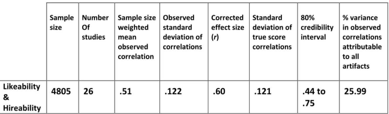
reliabilities was created. The Hunter & Schmidt procedure then calculates the amount of artifactual variance due to measurement error that is likely to be observed. While Paese and Switzer (1988) found that this procedure can slightly overestimate the amount of artifactual variance, this procedure is still useful in cases in which the reliability data is not available for all studies. Table 3.1 shows the basic results of this meta-analysis.
Table 3.1: Meta-analysis of correlations between likeability and hireability
Sample size Number Of studies Sample size weighted mean observed correlation Observed standard deviation of correlations Corrected effect size (r) Standard deviation of true score correlations 80% credibility interval % variance in observed correlations attributable to all artifacts Likeability & Hireability 4891 28 .52 .127 .60 .126 .44 to .76 25.05
0 0.1 0.2 0.3 0.4 0.5 0.6 0.7 0.8 0.9 1 2 3 4 5 6 7 8 9 10 11 12 13 14 15 16 17 18 19 20 21 22 23 24 25 26 27 28 Eff e ct Si ze E sti m ate s ( r )
Likeability has a strong positive correlation with hireability, .52 when uncorrected for artifacts, .60 when corrected for artifacts and sampling error. However, the percent of variance in the observed correlation attributable to all artifacts was much less than 75% (the percentage Schmidt & Hunter use as a cutoff) – it was only 25%. That means that moderators are very likely present.
The 80% credibility interval around the mean corrected effect size is also used to detect moderators. If it is large or includes zero, that suggests that it is not an estimate of the population correlation – the .44 to .76 credibility interval here did not contain zero but it was very wide. (Koslowsky and Sagie (1993) suggest using a rule of thumb of a
credibility interval of 0.11 to suggest the presence of a moderator.)
As recommended by Roth and Switzer (2002), the first analysis to attempt to adjust the accuracy of true likeability/hireability effect size was to look for potential outliers in the data set:
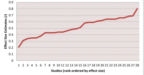
The correlations climbed a fairly gentle slope except at each end where they either jumped or dropped .10 (from .21 to .31 and from .69 to .80) These two endpoint studies could be outliers, and an analysis was run without them:
Table 3.2: Meta-analysis of correlations between likeability and hireability (no outliers)
Sample size Number Of studies Sample size weighted mean observed correlation Observed standard deviation of correlations Corrected effect size (r) Standard deviation of true score correlations 80% credibility interval % variance in observed correlations attributable to all artifacts Likeability & Hireability 4805 26 .51 .122 .60 .121 .44 to .75 25.99
The percent of variance in the observed correlation attributable to all artifacts only moved up to 25.99% from 25.05% – still a very long way from 75%, indicating that there was still a moderator.
According to Jose Cortina (2003), the 75% rule and 80% credibility interval taken together “would have the most power to detect moderators but would also have the highest Type I error rates by a considerable margin.” (p. 420). In order to reduce Type I error, a third moderator test was conducted on the set of effect sizes without the two outliers – a chi-square test of heterogeneity (Borenstein, Hedges, Higgins, and Rothstein, 2009). Its Q statistic (Q=66.9, p=.001) showed a significant amount of heterogeneity in the effect sizes, again strongly indicating a moderator or moderators.
No obvious moderators presented themselves in the coded items from the articles. It was thought that the use of a likeability measure across studies (particularly
the Interpersonal Judgment Scale) might result in a form of common method variance, but it did not dominate the studies or appear in any pattern among the correlations. Also considered as a possible subtle moderator was the cognitive ability load in the positions the selectors were hiring for – perhaps likeability was associated with less-complex clerical and sales positions. No support was found for this supposition either.
The moderator is continuous, not bimodal (see the relative smoothness of Figure 3.1) with “bands” of correlations around .40 and .60. Looking at the studies sorted by correlation (Appendix M), what those clusters of studies seem to have in common might be the selectors. Keenan (1978) looked at the relationship between likeability and interviewer experience – he found a correlation of .66 between likeability and overall employment suitability ratings made by experienced campus interviewers but only a correlation of .35 for inexperienced interviewers. Likewise in this meta-analysis, the student selectors were more likely to be in the lower cluster of studies and “real employees” and campus recruiters were in the upper band of studies. Also supporting experience as a moderator is the fact that experience is not binary, it’s continuous – one is not “inexperienced” then “experienced” but gains a continuing level of experience over time.
Without a larger collection of studies, a moderator analysis cannot be performed, but speculatively, selector experience may account for much of the unexplained variance. The hypothesis that the relationship between likeability and hiring would show “a
significant effect size” was somewhat supported – the 80% confidence interval is .44 to .75 but unknown moderators were present.
Study 2: Decision Study
Descriptive statistics for all variables in the decision study are included in Appendix N. A correlation matrix for all of the study variables is also included in Appendix O. One faculty participant asked that his data be excluded from the study and his responses were deleted from the survey website before results were downloaded; he was not included in any participant count. All faculty, staff, or graduate student
respondents answered that they had at least glanced over the letters of recommendation, so none were excluded for not being exposed to the experimental manipulation. Primary data analysis was conducted only on faculty participants (the small number of responses by graduate students and staff was treated just as exploratory data.) The response rate for faculty was 15.2%; 112 of the 735 faculty contacted completed the survey.
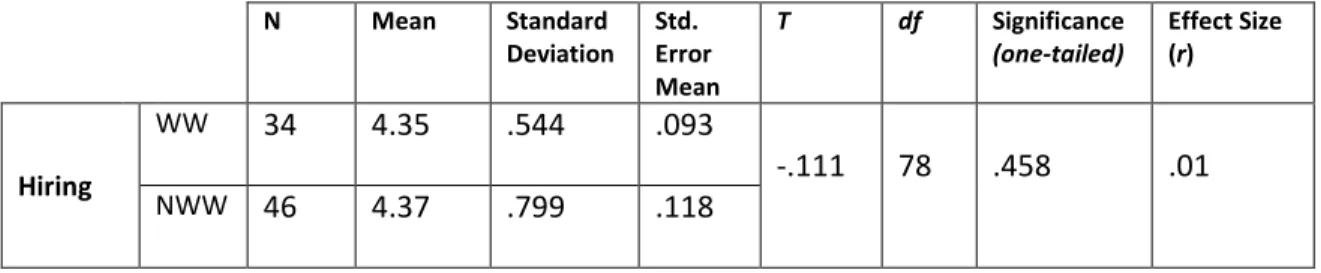
The hypothesis that there would be lower hiring recommendation ratings for the candidate in the “working with” (WW) than in the “not working with” (NWW)
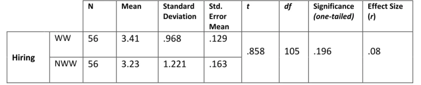
conditions was first examined using a t-test on the hiring recommendation question (Table 3.3). On average, faculty actually recommended more strongly to hire the candidate in the condition where they would be working with the candidate (M=3.41, SE=.129) than in the condition where they would not be working with him (M=3.23, SE=.163). This difference was not significant t(105)=.858, p=.196.
Table 3.3: t-test of hiring recommendations in the “working with” and “not working with” conditions N Mean Standard Deviation Std. Error Mean t df Significance (one-tailed) Effect Size (r) Hiring WW 56 3.41 .968 .129 .858 105 .196 .08 NWW 56 3.23 1.221 .163
In order to make the strongest possible attempt to find an effect, both the hiring and interview recommendation questions were combined in a MANOVA. Using Hotelling’s trace statistic, there was still not a significant effect of whether the faculty selectors would work with the candidate or not on their recommendations of hiring and interviewing the candidate, T=.015, F(2,109) = .837, p=.436 (All the multivariate tests were essentially identical – Hotelling’s is reported because of its robustness in two-group situations when sample sizes are equal (Hakstian, Roed & Lind, 1979).
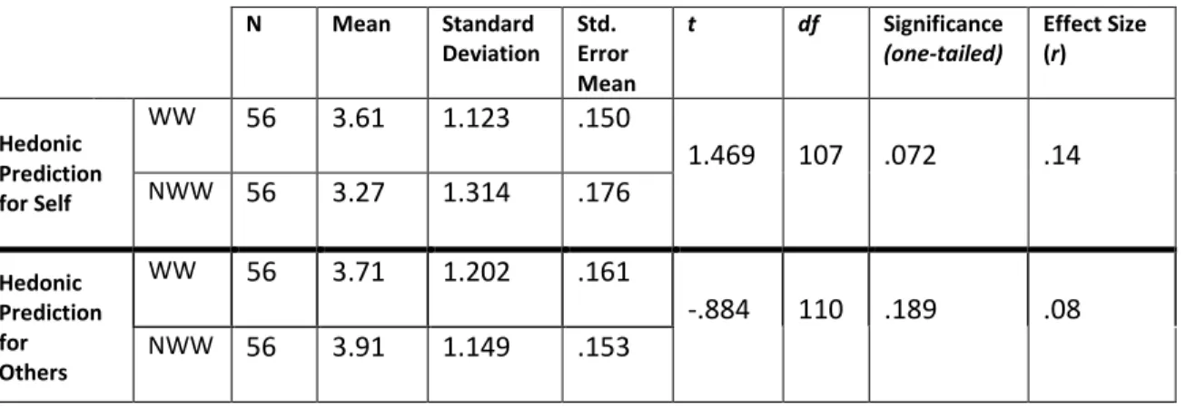
The hypothesis of a lesser likelihood of reporting a hedonic prediction in the NWW condition than the WW condition was resolved by a t-test between the hedonic prediction self-report and the NWW/WW groups (Table 3.4). On average, faculty did respond that they thought about how the candidate would affect their future happiness to a greater extent under the WW condition (M=3.61, SE=.150) than under the NWW condition (M=3.27, SE=.176). This difference, however, was not significant t(107)=1.469, p=.072.
Table 3.4: t-test of hedonic predictions for self and others in the “working with” and “not working with” conditions N Mean Standard Deviation Std. Error Mean t df Significance (one-tailed) Effect Size (r) Hedonic Prediction for Self WW 56 3.61 1.123 .150 1.469 107 .072 .14 NWW 56 3.27 1.314 .176 Hedonic Prediction for Others WW 56 3.71 1.202 .161 -.884 110 .189 .08 NWW 56 3.91 1.149 .153
There was even less support for the idea that faculty would make significantly more hedonic predictions for others in the “not working with condition” (M=3.91, SE=.153) than in the “working with” condition (M=3.71, SE=.161). The direction of the effect was correctly predicted, t(110)= -.884, p=.189, but the effect size was negligible (.08).
The final research hypothesis in the decision study predicted that the candidate would be rated higher on job skills by selectors (and would receive fewer negative comments) in the “not working with” condition than in the “working with” condition. This prediction was based on the assumption that there would be a significantly positive difference in the selection rate for the candidate in the “not working with condition” compared to the “working with condition” – an unsupported hypothesis. It was theorized that by making the candidate’s positive ratings more positive and “negative” ratings less negative in the NWW condition and downgrading ratings in the WW condition, selectors would rationalize their hiring decision and reduce dissonance. A MANOVA was computed for the five job criteria taken from the position description
across both conditions; using Pillai’s trace, there was no significant effect shown for skill rating across conditions, V=.071, F(5,103)=1.567, p=.176.
Faculty comments were also considered across conditions; with such a small text sample only a cursory evaluation could be employed. The question “What do you think working with this person would be like?” received many mixed responses such as “It would not be a pleasant experience but it sounds like it would accomplish the objective of getting funding”; “Profitable but painful”; and “Miserable, he sounds like a jerk, but he gets the results done.”
In order to explore these faculty comments, another subset of participants was created – those who strongly or somewhat disagreed that the candidate should be hired:
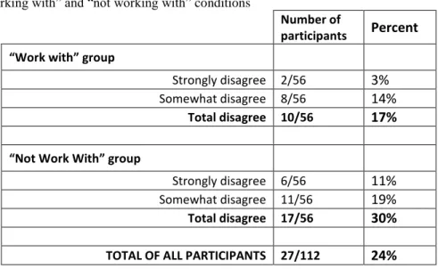
Table 3.5: Total of faculty participants who disagree with hiring candidate across “working with” and “not working with” conditions
Number of
participants Percent “Work with” group
Strongly disagree 2/56 3%
Somewhat disagree 8/56 14% Total disagree 10/56 17% “Not Work With” group
Strongly disagree 6/56 11%
Somewhat disagree 11/56 19% Total disagree 17/56 30%
TOTAL OF ALL PARTICIPANTS 27/112 24%
This subgroup makes up 24% of the faculty respondents and will hereinafter be referred to as the “24% group” (and the “76% group” is the percentage of the faculty who
agreed to hire the candidate or were neutral). The comments from the “Work With” (WW)/”Not Work With” (NWW) and the 24%/76% groups were examined using two different tools. The first was a word frequency counter. The comments from the
subgroups were separately copied into a web application (WriteWords, 2012) to calculate the occurrence of each word in the comments.
The word frequencies for each subgroup were then compared to two different word lists. The first was a list of “emotion words” taken from the Linguistic Inquiry and Word Count (LIWC) Dictionary (Pennebaker, Booth, & Francis, 2007), supplemented by a number of relevant words that the participants had used to describe the candidate in an emotional way. (The emotion word list and frequency counts are in Appendix P.) The second list consisted of “job performance words” that were also selected from the
comments as those most specifically relevant to describing the candidate’s potential work in the described position. (The job performance word list and frequency counts are in Appendix Q.)
The faculty in both experimental conditions (“work with” or “not work with”) used equal numbers of emotion words and job performance words. When counting emotion words, WW=103 versus NWW= 109; for job performance words, WW=173 versus. NWW=171. The 24% group who did not want to hire the candidate, however, made more emotional comments that the 76% group – they used 62 emotional words (2.3 per person) vs. 150 for the 76%ers (1.7 per person). The 24% group also used more job performance words than the other group – 3.5 per person versus 2.9.
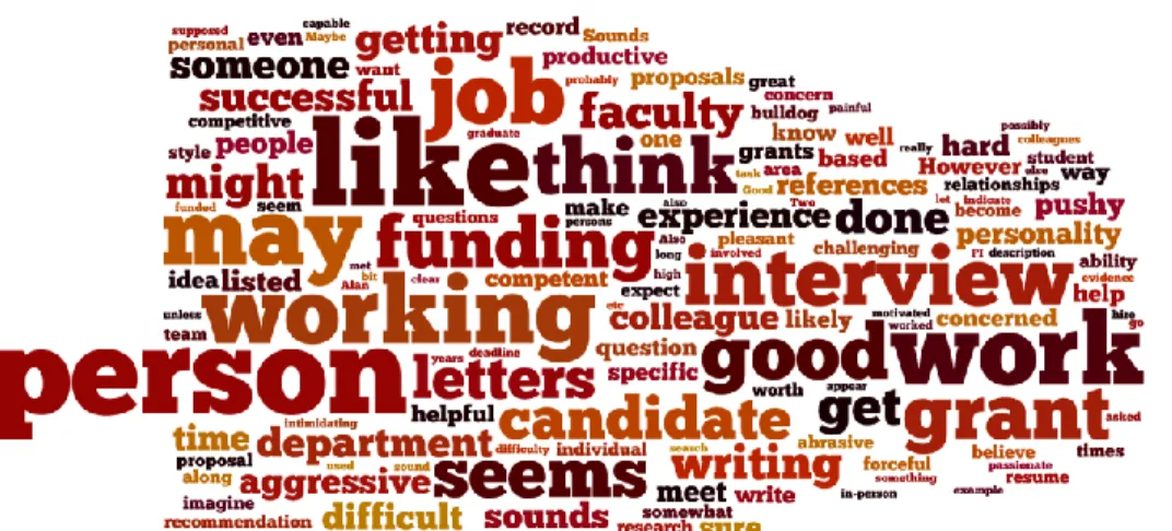
The other tool is a type of frequency counter, but the output is a “word cloud” where the size and boldness of the word reflects its frequency in the text. A word cloud was created for the “24% group” and one for the remaining faculty participants, using the Wordle application (Feinberg, 2011).
Figure 3.2: Word cloud of comments from faculty participants who disagree with hiring candidate across “working with” and “not working with” conditions (the 24% group)
Figure 3.3: Word cloud of comments from faculty participants who were neutral or agreed or strongly agreed that the candidate should be hired (across “working with” and “not working with” conditions) (the 76% group)
The words “aggressive” and “horrible” and “stressful” are more prominent in Figure 3.2 than in Figure 3.3; the words “successful,” “grant,” and “funding” are certainly more prominent in Figure 3.3 than Figure 3.2. (With both methods, of course, one must consider the meaning of single words taken out of context – “not necessarily pleasant” and “probably pleasant” are not the same thing.)
Other survey respondents
The faculty were the primary targets of the study, but the survey was also sent to academic department staff and graduate students. Only 12 staff members out of the 130 contacted (9.2%) completed the survey, a response too small to be effectively analyzed.
The 30 graduate student responses were, however, used to examine the primary hypothesis that there would be lower hiring recommendation ratings for the candidate in the “working with” (WW) than in the “not working with” (NWW) conditions. (The graduate student response rate was the lowest – 7.8% – 385 students received a
recruitment email.) Results of t-tests on both the hiring recommendation question and the interview recommendation question are shown in Table 3.6. On average, unlike the faculty, graduate students did recommended more strongly to hire the candidate in the condition where they would be not be working with the candidate (M=3.94, SE=.266) than in the condition where they would be working with him (M=3.71, SE=.163), but this difference was not significant t(24) = -.716, p=.241. The graduate students in the WW condition recommended more strongly to interview the candidate (M=4.79, SE=.214) that did the students in the NWW condition (M=4.50, SE=.289); this difference was not