Q
ED
Queen’s Economics Department Working Paper No. 1278
Bootstrap Confidence Sets with Weak Instruments
Russell Davidson
McGill University
James G. MacKinnon
Queen‘s University
Department of Economics
Queen’s University
94 University Avenue
Kingston, Ontario, Canada
K7L 3N6
Bootstrap Confidence Sets
with Weak Instruments
by
Russell Davidson
Department of Economics and CIREQMcGill University Montr´eal, Qu´ebec, Canada
H3A 2T7
GREQAM
Centre de la Vieille Charit´e 2 Rue de la Charit´e
13236 Marseille cedex 02, France [email protected]
and
James G. MacKinnon
Department of EconomicsQueen’s University Kingston, Ontario, Canada
K7L 3N6 [email protected]
Abstract
We study several methods of constructing confidence sets for the coefficient of the single right-hand-side endogenous variable in a linear equation with weak instru-ments. Two of these are based on conditional likelihood ratio (CLR) tests, and the others are based on inverting t statistics or the bootstrap P values associated with them. We propose a new method for constructing bootstrap confidence sets based on t statistics. In large samples, the procedures that generally work best are CLR confidence sets using asymptotic critical values and bootstrap confidence sets based on LIML estimates.
Key words: Weak instruments, bootstrap, confidence sets JEL codes: C10, C15
This research was supported, in part, by grants from the Social Sciences and Humanities Research Council of Canada, the Canada Research Chairs program (Chair in Economics, McGill University), and the Fonds Qu´eb´ecois de Recherche sur la Soci´et´e et la Culture.
1. Introduction
Inference in the linear simultaneous equations model is notoriously difficult when the instruments are weak. Although there has been an enormous amount of work on this topic since the seminal paper of Staiger and Stock (1997), much of it has focused on the properties of estimators (especially their bias) and on the properties of test statistics. Despite important work by Zivot, Startz, and Nelson (1998), Mikusheva (2010),1 and many others, there does not yet appear to be a consensus on the best way to construct confidence sets when instruments are weak. This paper examines several procedures that are either easy to use and popular or may be expected to perform well. We obtain a number of striking results.
In principle, one can construct a confidence set by inverting any suitable test statistic, possibly after it has been bootstrapped in some way. For the linear simultaneous equations model, the natural candidates are Wald (that is, t) tests, likelihood ratio (LR) tests, Lagrange multiplier (LM) tests, and the Anderson-Rubin (AR) test. Partly for reasons of space and readability, we restrict attention to confidence sets that are based on Wald tests or on the conditional LR (CLR) test of Moreira(2003). We consider Wald-based confidence sets because they are the most commonly used in practice and because, contrary to what is widely believed, it is possible to make them perform well when the instruments are weak by using certain bootstrap methods. We consider CLR confidence sets because the CLR test often seems to perform very well and because the results of Mikusheva (2010) suggest that CLR confidence sets also perform well.
We do not consider confidence sets based on the LM test or the closely related test of Kleibergen (2002) because the results of Mikusheva (2010) are not at all encouraging. It is partly for the same reason that we do not consider confidence sets based on the AR test of Anderson and Rubin(1949). More importantly, as was shown in Davidson and MacKinnon(2011), AR confidence sets have many undesirable properties. Although their unconditional coverage is, under classical assumptions, always correct, their coverage conditional on being bounded intervals can be far from correct. Moreover, the lengths of AR intervals, when they exist, provide grossly unreliable information about the precision with which the parameter of interest has been estimated.
In the next section, we discuss the basic model and some conventional procedures, both asymptotic and bootstrap, for constructing Wald-based confidence intervals. In Section 3, we discuss a new procedure for constructing Wald-based bootstrap confidence intervals. In Section 4, we discuss confidence sets based on the CLR test. In Section 5, we present a number of simulation results, some of which may be quite surprising. In Section 6, we summarize our conclusions.
2. Wald-Based Confidence Intervals
We restrict attention to the two-equation linear model
y1 =βy2+Zγ+u1 (1)
y2 =Wπ+u2 =Zπ1+W2π2+u2. (2) Here y1 andy2 are n--vectors of observations on endogenous variables, Z is an n×k matrix of observations on exogenous variables, andW is ann×l matrix of exogenous instruments with the property thatS(Z), the subspace spanned by the columns ofZ, lies inS(W), the subspace spanned by the columns ofW. Then×(l−k) matrix W2 is constructed in such a way that S(Z,W2) = S(W). Equation (1) is a structural equation, and equation (2) is a reduced-form equation. The parameter of interest is β, the coefficient on y2 in equation (1).
The disturbance vectors u1 and u2 are assumed to be serially uncorrelated and homoskedastic, with mean zero and contemporaneous covariance matrix
Σ ≡ σ2 1 ρσ1σ2 ρσ1σ2 σ22 .
We assume that the model is either exactly identified or overidentified, which implies thatl ≥k+ 1. The number of overidentifying restrictions is l−k−1.
Equations (1) and (2) can be estimated in many ways. We restrict attention to the two most common single-equation methods, namely, generalized instrumental variables (IV), which is numerically identical to two-stage least squares, and limited-information maximum likelihood (LIML). The two estimators ofβare, in self-evident notation, ˆβIV and ˆβLIML, and their standard errors are ˆsIV and ˆsLIML.
The simplest and most natural way to form a confidence interval for β in (1) is to invert thet statistic forβ =β0, which is the signed square root of the Wald statistic. This yields the asymptotic Wald intervals
[ ˆβIV−Φ1−α/2ˆsIV, βˆIV+ Φ1−α/2ˆsIV] (3) and
[ ˆβLIML−Φ1−α/2sˆLIML, βˆLIML+ Φ1−α/2sˆLIML], (4) where Φ1−α/2 denotes the 1−α/2 quantile of the standard normal distribution. How-ever, as is well-known and will be seen again in Section 5, these intervals often have poor finite-sample properties when the instruments are weak. This is particularly true for (3), in part because ˆβIV can be severely biased in that case.
A natural way in which to attempt to obtain more reliable Wald intervals is to use the bootstrap. The oldest, and conceptually the simplest, bootstrap method for the linear simultaneous equations model is the pairs bootstrap, which was proposed by Freed-man (1984). The idea is simply to resample the rows of the matrix [y1 y2 Z W2].
Each such bootstrap sample, indexed by j = 1, . . . , B, is then used to compute a bootstrapt statistic t∗j = βˆ ∗ j −βˆ s( ˆβ∗ j) ,
where ˆβ could be either ˆβIV or ˆβLIML, ˆβj∗ is the corresponding estimate from the jth bootstrap sample, and s( ˆβ∗
j) is the standard error of ˆβj∗. Using either ˆβIV and ˆsIV or ˆβLIML and ˆsLIML, together with the B values of t∗j, one then constructs an equal-tail percentile t confidence interval (also called a studentized bootstrap confidence interval) in the usual way; see, among many others, Davison and Hinkley (1997) or Davidson and MacKinnon(2004, Chapter 5). In the IV case, the interval is
[ ˆβIV−c∗1−α/2sˆIV, βˆIV−c∗α/2sˆIV], (5) where c∗
α/2 and c∗1−α/2 denote the estimated α/2 and 1−α/2 quantiles of the t∗j. When B= 999 and α= 0.05, for example, these are just numbers 25 and 975 in the list of the t∗
j sorted from smallest to largest.
The Wald-based intervals (3), (4), and (5) are easy to construct and commonly used, but they cannot possibly have correct coverage when the instruments are weak, because they cannot be unbounded. When the instruments in a linear simultaneous-equations model are sufficiently weak, a confidence set with correct coverage must be unbounded with positive probability; see Gleser and Hwang (1987) and Dufour (1997). Unlike these Wald-based intervals, the confidence sets discussed in the next two sections can be unbounded with positive probability.
3. RE Bootstrap Confidence Sets
In Davidson and MacKinnon (2008), we proposed the restricted efficient, or RE, bootstrap in the context of hypothesis tests on β in equation (1). In this section, we discuss how the RE bootstrap can also be used to form confidence sets. The simulation results of Section 5 suggest that confidence sets based on the RE bootstrap generally perform quite well, at least when the instruments are not very weak. The main disadvantage of these confidence sets is that they are relatively complicated and expensive to compute.
The RE bootstrap has two key features. The bootstrap DGP is conditional on a particular value of β (hence “restricted”), and it uses an efficient estimate of π
(hence “efficient”). For any specified value β0, we can run regression (1) to obtain parameter estimates ˜γ and residuals ˜u1. The latter may be rescaled by multiplying them by a factor of (n/(n−k))1/2. We then run the regression
y2 =Wπ+δu˜1 + residuals. (6) This yields parameter estimates ˜π and adjusted residuals ˜u2 ≡y2−Wπ˜. The latter should be rescaled by multiplying them by a factor of (n/(n−l))1/2. It can be shown
that ˜π is asymptotically equivalent to the estimate one would obtain by using FIML or 3SLS. This estimate was used by Kleibergen (2002) in a different context. In addition, Moreira(2009) explains why using ˜π rather than any other estimator ofπ
leads to a version of the LM test of the hypothesis thatβ =β0 that is asymptotically similar with weak instruments. See also Moreira, Porter, and Suarez (2009), where bootstrap validity is shown for that version of the LM test.
Generating a bootstrap sample using the RE bootstrap is quite simple. We form two vectors of bootstrap disturbances, u∗
1 and u∗2, with elements u∗i1 and u∗i2 for i = 1, . . . , n, resampled from the pairs of rescaled residuals, that is, from the joint empirical distribution of the rescaled residuals. We then set
y2∗ =Wπ˜ +u∗2, and
y1∗ =β0y∗2+Zγ˜+u∗1.
(7) If we generateB bootstrap samples, we can compute an equal-tail bootstrapP value for the hypothesis thatβ =β0. It is simply
ˆ p∗(β0) = 2 B min B X j=1 I(τj∗ <τˆ), B X j=1 I(τj∗ ≥τˆ) ! , (8)
where I(·) is the indicator function, ˆτ = ( ˆβ−β0)/s( ˆβ), andτj∗ = ( ˆβj∗−β0)/s( ˆβj∗). Here ˆ
β may denote either ˆβIV or ˆβLIML, and ˆβj∗ then denotes the corresponding estimate for the jth bootstrap sample. It is important to calculate the standard errors s( ˆβ) and s( ˆβ∗
j) in the same way. By using the equal-tail P value (8), we do not impose symmetry on the distribution ofτ.
Using the RE bootstrap to obtain a confidence set is a bit complicated. Consider the upper limit, ˆβu. Start with an initial estimate, say ˆβu1 (one obvious candidate is the upper limit of the asymptotic confidence interval) and compute ˆp∗( ˆβ1
u) using equation (8). If ˆp∗( ˆβ1
u)> α, then ˆβu1 is too small; if ˆp∗( ˆβu1)< α, then it is too large. Try another candidate, say ˆβ2
u, which must be larger than ˆβu1 in the former case and smaller in the latter case. Calculate ˆp∗( ˆβ2
u) and repeat if necessary. The way in which ˆ
β2
u is chosen may have a significant impact on computational cost, but it should have no effect on the properties of the RE bootstrap confidence set.
If, aftermtries, we have found ˆβm−1
u and ˆβumsuch that ˆp∗( ˆβum−1)−αand ˆp∗( ˆβum)−α have opposite signs, then ˆβu must lie between them. At this point, various numerical methods can be used to find it. Since ˆp∗(β
0) is not differentiable, we must use a method that does not need derivatives. In our simulations, we use bisection, which is easy to program and reasonably fast. Note that exactly the same set of random numbers must be used for every set ofB bootstrap samples. Otherwise, the value of ˆ
p∗(β
0) would be different each time we evaluated it.
The procedure for finding the lower limit, ˆβl, is essentially the same as the one for finding the upper limit, with obvious changes in sign at various points.
In the above description of the algorithm, we have implicitly assumed that, if β0 is sufficiently large or sufficiently small, ˆp∗(β
0) must be less than α. However, that is not always true. The confidence set has no upper bound ifp∗(β
0)> α asβ0 tends to plus infinity, and it has no lower bound if p∗(β
0) > α as β0 tends to minus infinity. In practice, we may reasonably conclude that the confidence set is unbounded from above (below) if p∗(β
0)> α for a very large positive (negative) value of β0.
Unbounded confidence sets can occur as a consequence of the fact, shown in Davidson and MacKinnon (2008), that, for weak enough instruments, the distribution of the tstatistic for a test ofβ = 0 when the trueβis indeed zero overlaps the distribution in the limit in which β tends to infinity. Thus the bootstrap distribution of a statistic that tests a true hypothesis can overlap the distribution of a statistic that tests a hypothesis that assigns a value to β arbitrarily far from the true value, if the instruments are sufficiently weak.
RE bootstrap confidence sets may contain holes. In fact, simulations suggest that they frequently contain a hole when they are unbounded. It is therefore important to check for holes and for unboundedness even if the procedure described above has apparently located both ˆβu and ˆβl. If there are values of β0 greater than ˆβu or less than ˆβl for which p∗(β0) > α, it is easy enough to locate the other end of the hole. However, we do not recommend using unbounded confidence sets to make inferences. The fact that a confidence set is unbounded strongly suggests that the instruments are so weak as to make reliable inference impossible.
The fact that RE bootstrap confidence sets may be unbounded (and in fact often are unbounded when the instruments are very weak) is actually a desirable feature, as we noted at the end of the preceding section; see Gleser and Hwang (1987)and Dufour (1997). Because RE bootstrap confidence sets can be unbounded, it is possible for them to have very good coverage.
Unless heteroskedasticity is clearly absent, it is generally wise to use confidence sets that are robust to it. One advantage of using confidence sets based on t statistics is that it is very easy to do so. We simply replace the ordinary t statistic with one based on a heteroskedasticity-consistent standard error and employ a slightly modified version of the RE bootstrap.
The wild restricted efficient, or WRE, bootstrap was proposed by Davidson and MacKinnon (2010). It is very similar to the RE bootstrap, except that the ith pair of rescaled residuals is always associated with the ith observation. To generate the bootstrap disturbances, we simply multiply each pair of rescaled residuals by a random variable v∗
i with mean zero and variance one. See Davidson and Flachaire (2008)for more about the wild bootstrap. In samples of reasonable size (more than a few hundred observations) with heteroskedastic disturbances, this should work just about as well as using ordinary standard errors and the RE bootstrap when the disturbances are actually homoskedastic.
4. CLR Confidence Sets
Because the CLR test of Moreira(2003)seems to work better than other asymptotic tests for the value ofβ, it is natural to consider confidence sets obtained by inverting CLR tests. Mikusheva (2010) discusses confidence sets of this type. In this section, we present a different derivation which emphasizes computational issues.
The CLR test statistic and all associated quantities, including ˆβIV, ˆβLIML, and their standard errors, depend on the data only through the six quantities
P11 ≡y1>P1y1, P12 ≡y1>P1y2, P22 ≡y2>P1y2,
M11 ≡y1>MWy1, M12 ≡y1>MWy2, and M22 ≡y2>MWy2,
(9) whereMW ≡I−W(W>W)−1W>,P1 ≡MZ−MW, andMZ ≡I−Z(Z>Z)−1Z>.
These six quantities just depend on sums of squared residuals and/or sums of cross-products of residuals from the regressions ofy1 and y2 on Z and W.
In order to compute the CLR test statistic for the hypothesis that β = β0, we also need the quantities
Q11 ≡P11−2β0P12+β02P22, Q12 ≡P12−β0P22, Q22 ≡P22,
N11 ≡M11−2β0M12+β02M22, N12 ≡M12−β0M22, and N22 ≡M22.
(10) From these, we calculate
SS(β0)≡nQ11/N11, (11) ST(β0)≡ n ∆1/2 Q12− Q11N12 N11 , and (12) T T(β0)≡ n ∆ Q22N11−2Q12N12+ Q11N 2 12 N11 , (13) where ∆≡N11N22−N122 =M11M22 −M122 . (14) It is easy to verify that ∆ does not depend on β0. In Mikusheva (2010), it is shown that the eigenvalues of the 2×2 matrix
SS(β0) ST(β0) ST(β0) T T(β0)
also do not depend on β0. These eigenvalues are
1 − 2 SS(β0) +T T(β0)± q SS(β0)−T T(β0) 2 + 4ST2(β 0) . It follows thatI1 ≡SS(β0) +T T(β0) and I2 ≡
SS(β0)−T T(β0) 2 + 4ST2(β 0) 1/2 are also independent of β0.
The LR statistic for testing the hypothesis thatβ =β0 takes the form LR(β0) =n log 1 +SS(β0)/n −n log 1 + (I1−I2)/2n ; (15) see, among others, Davidson and MacKinnon (2008). The LR statistic depends on β0 only through SS(β0). The concentrated loglikelihood function for model (3) is a deterministic, decreasing, function of SS(β0). It is therefore maximized by minimizingSS(β0), for which the minimizer is ˆβLIML. It follows that the LR statistic is also minimized atβ0 = ˆβLIML and that LR( ˆβLIML) = 0.
Moreira (2003) and Mikusheva (2010) simplify the LR statistic (15) by Taylor ex-panding the logarithms and discarding terms that tend to zero as n → ∞. This yields
LR0(β0) =−12 SS(β0)−T T(β0) +I2
=M −T T(β0), (16) whereM ≡ 1
2(I1+I2). The rightmost expression in (16) tells us thatT T( ˆβLIML) =M and that LR0( ˆβLIML) = 0. This implies that ˆβLIML belongs to any confidence set found by inverting the test based on LR0(β0).
The idea behind the CLR test is that, even though LR0(β0) is not pivotal with weak instruments, its distribution conditional on T T(β0) is asymptotically pivotal. This distribution can be estimated in various ways. We discuss two of them, one based on asymptotic theory and one based on the pairs bootstrap, in the Appendix. For now, we simply let F ·, T T(β0)
denote the estimated cumulative distribution function (CDF) of LR0(β0) conditional on T T(β0), and let cα denote the 1−α quantile of that CDF.
The P value for the hypothesis β = β0 is 1 − F LR0(β0), T T(β0)
, and so the confidence set at nominal confidence level 1−α is
β0|1−F LR0(β0), T T(β0)
> α . (17)
Using (16), we can replace LR0(β0) by M−T T(β0). The inequality inside the braces in (17) can then be rearranged as
F M −T T(β0), T T(β0)
≤1−α. (18)
It is shown in the Appendix that, for given M, the function F(M −c, c) decreases monotonically for 0 ≤ c ≤ M. This implies that the equation F(M −c, c) = 1−α has a unique solutioncα ∈[0, M] for givenα and M, provided thatα > 1−F(M,0). BecauseF(M −c, c) is decreasing in c, it follows that the inequality (18) is satisfied for all β0 such that T T(β0)≥cα.
The values ofβ0 that satisfy the inequalityT T(β0)≥cα can now be found. By using the Qij and Nij from (10) in the definition of T T(β0), it can be seen after some algebra that T T(β0) = n ∆ Aβ2 0 −2Bβ0+C M22β02−2M12β0+M11 ,
where
A=P22M122 −2P12M12M22+P11M222 ,
B=P22M11M12−P12M11M22−P12M122 +P11M12M22, and C =P22M112 −2P12M11M12+P11M122 .
(19) The inequality T T(β0)≥cα is then equivalent to the quadratic inequality
1 −nM22∆cα−A β02−2 −n1M12∆cα−B β0+−n1M11∆cα−C ≤0. (20)
Except for notational differences, this inequality is the same as that given following Lemma 1 in Mikusheva (2010).
Observe that, sinceT T(β0) is positive, all real values ofβ0 must satisfy the inequality T T(β0)≥0, so that, when cα = 0, the confidence set is the entire real line, R. As is shown in the Appendix, there always exists α small enough that the confidence set is R. If α is so small that the inequality α > 1−F(M,0) is not satisfied, then the confidence set is againR.
If the quadratic equation that sets the left-hand side of (20) to zero has real roots, they are b± = M12∆cα/n−B M22∆cα/n−A ±√D, where (21) D≡ (M12∆cα/n−B) 2 (M22∆cα/n−A)2 − M11∆cα/n−C M22∆cα/n−A . (22)
If D here is negative, then the left-hand side of (20) is either everywhere positive or everywhere negative. But if it is positive, then (20) cannot be satisfied, which would imply an empty confidence set, contrary to the fact already established that the LIML estimate ˆβ always belongs to the confidence set for any α. This implies that, if D <0, then the coefficient M22∆cα/n−A in (20) must also be negative. IfD >0, theb±are the boundary points of the confidence set. IfM22∆cα/n−A >0, the set is the bounded interval [b−, b+]. If M22∆cα/n−A < 0, it is the real line with a hole in it, the hole being the same bounded interval. In the knife-edge case in whichM22∆cα/n−A = 0, the confidence set is an unbounded interval which may be open either to the left or to the right, depending on the signs of the other coefficients in (20).
We now set out explicitly an algorithm for constructing CLR confidence sets.
1. Compute the six quantities defined in (9) and use them to calculate the quantities A, B, and C defined in (19).
2. ComputeM =T T( ˆβLIML) using (10), (11), (12), (13), and (14).
3. Obtain either the asymptotic or pairs bootstrap critical value cα using one of the procedures discussed in the Appendix.
4. Evaluate D defined in (22). If D <0, the confidence set isR.
5. If D >0, compute b− and b+ using (21). If M22∆cα/n−A > 0, the set is the bounded interval [b−, b+]. Otherwise (ignoring the knife-edge case), it is the real line except for the bounded interval [b−, b+].
Note that the CLR confidence set, when it is a bounded interval, is not centered at ˆ
βLIML, although, as we have seen, it must always contain ˆβLIML. 5. Simulation Evidence
Following Davidson and MacKinnon (2008), we use the DGP:
y1 =βy2+u1,
y2 =aw+u2,
(23) wherew ∈S(W) is an n--vector with kwk2 = 1, and
u1 =rv1+ρv2, u2 =v2, v1 v2 ∼N(0,I), r2+ρ2 = 1. (24)
It may seem curious that there is just a single instrumentw in the DGP when there are l of them in equation (2). But the only property of W that matters is S(W), the subspace spanned by the columns of W. In effect, we have performed a linear transformation on W so that all of the explanatory power comes from the vector w
and the other columns ofW are simply noise. Of course, such a transformation has no effect on S(W).
By normalizing the instrument vector w to have squared length unity, that is,
w>w= 1, we are implicitly using weak-instrument asymptotics; see Staiger and Stock (1997). The strength of the instruments is measured by the parameter a, the square of which is the scalar concentration parameter; see Phillips(1983, p. 470) and Stock, Wright, and Yogo (2002). Because we are only concerned with confidence sets, the error variances have all been normalized to unity, which is something we could not do if we were concerned with bias.
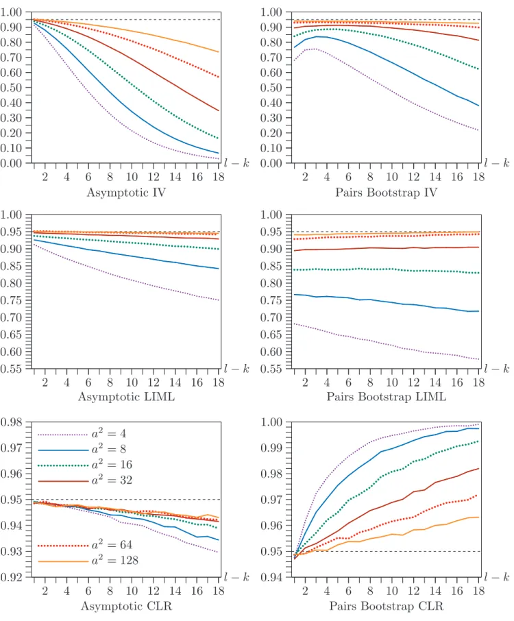
The first three figures each contain six panels, two for each of the IV Wald, IV LIML, and CLR confidence sets. In all cases, the left-hand panel of each pair shows coverage for asymptotic 95% confidence sets (which are based on the standard normal distribution for the two Wald intervals), and the right-hand panel shows coverage for 95% confidence sets based on the pairs bootstrap. Asymptotic results are based on 500,000 replications, and bootstrap results are based on 100,000 replications, each withB = 999 bootstrap samples.
Figure 1 shows the effect of varying the number of instruments that are not also regressors in the structural equation, that is,l−k, for six values of a2. The six values are 4, 8, 16, 32, 64, and 128, and l−k varies from 1 to 18. The sample size is fairly
large (n= 400), and the correlation between the structural and reduced-form errors is quite high (ρ= 0.8).
For the asymptotic IV Wald intervals, there is generally severe undercoverage unless l−k is small anda2 is large. The pairs bootstrap generally helps somewhat, except when l−k is small. For the bootstrap intervals, undercoverage is moderate when a2 ≥64 and l−k ≤10, but it is still severe in most cases.
The asymptotic LIML Wald intervals always work better than the corresponding asymptotic IV ones. Undercoverage is nonexistent or quite moderate when a2 ≥64 for all values of l−k. However, the pairs bootstrap actually makes undercoverage worse, especially for small values of a2.
The asymptotic CLR confidence sets perform extremely well. They always under-cover, but only very slightly when l −k is small. The undercoverage gradually increases asl−k increases, especially whena2 is small, but it is never very great. In contrast, the pairs bootstrap CLR confidence sets almost always overcover, and they do so severely when a2 is small and l−k is large.
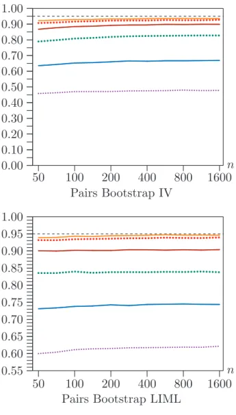
Figure 2 shows the effect of changing the sample size for l−k = 10, ρ = 0.8, and the same six values of a2. The sample sizes are 50, 70, 100, 141, 200, 282, 400, 565, 800, 1131, and 1600; each of these is approximately √2 times its predecessor. The performance of all the Wald intervals is strikingly insensitive to sample size. There tend to be slight improvements in coverage as n increases, which is most noticeable for a2 = 128.
In contrast, the performance of the CLR confidence sets depends greatly on the sample size. The undercoverage of the asymptotic CLR confidence sets diminishes rapidly as n increases. The overcoverage of the pairs bootstrap CLR intervals also diminishes, but less rapidly, especially for the smaller values of a2.
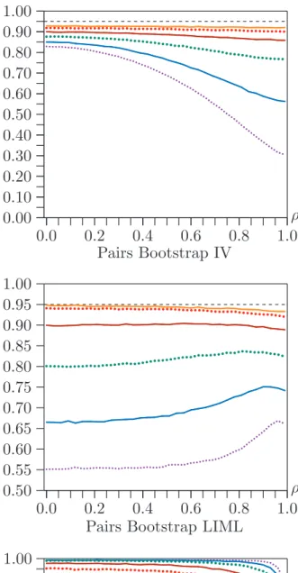
Figure 3 shows the effect of changing ρ. For the asymptotic results, there are 100 values between 0.00 and 0.99 increasing by 0.01. For the bootstrap results, there are 34 values between 0.00 and 0.99 increasing by 0.03. The sample size is 50, and l−k = 10.
Coverage of all the confidence sets depends strongly on ρ, except sometimes when a2 is large. This is most true for the asymptotic IV Wald intervals, which actually overcover for botha2 andρ small, even though they undercover very severely for a2 small and ρ large. As in Figure 1, the pairs bootstrap generally improves coverage for IV Wald intervals (but not when ρ is small). However, except when a2 is large, it actually causes LIML Wald intervals to undercover more severely.
The CLR confidence sets are only moderately sensitive to ρ. They do not perform particularly well in Figure 3, because the sample size is only 50. Based on the results in Figure 2, we can be confident that the undercoverage of asymptotic CLR intervals would be very much less severe if n were substantially larger.
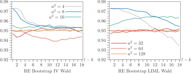
Figure 4 shows the coverage of RE bootstrap confidence sets based on both IV and LIML t statistics for the same case as Figure 1, that is, ρ = 0.80,n= 400, andl−k
varying between 1 and 18. Note the scale of the vertical axis. Although coverage is certainly not perfect, it is vastly better than for the asymptotic and pairs bootstrap Wald intervals. For larger values of l −k and a2, it is even better than for the asymptotic CLR confidence sets.
Figure 5 shows the coverage of RE bootstrap confidence sets for the same case as Figure 2, that is, ρ = 0.80, l −k = 10, and n varying between 50 and 1600. Once again, coverage is vastly better than for the asymptotic and pairs bootstrap Wald intervals. It is also better than the coverage of the CLR confidence sets for most sample sizes, but not for the largest sample sizes whena2 is small.
The results for the IV and LIML cases in Figure 5 are often quite different, and there are a few results that are hard to explain. The LIML confidence sets all work essentially perfectly for n ≥200 and a2 ≥ 32. However, it is only for a2 ≥128 that we can make a similar statement for the IV confidence sets. Not coincidentally, all of the LIML confidence sets for n ≥ 200 are bounded for a2 ≥ 64, and nearly all are bounded when a2 = 32, while a significant fraction of the IV confidence sets are unbounded even when a2 = 64.
Figure 6 shows the coverage of RE bootstrap confidence sets for the same case as Figure 3, that is,n= 50, l−k = 10, and ρ varying from 0.00 to 0.99 by 0.03. Once again, coverage is very much better in most cases than it was in Figure 3. As ρ increases, coverage generally deteriorates, especially for very large values of ρ in the LIML case when a2 ≤16.
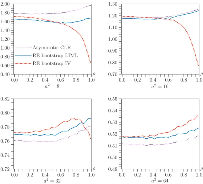
Figures 7 and 8 report results from a different set of experiments in which n = 400 andl−k = 2. Thus the sample size is fairly large, and there is only one overidentifying restriction. This is a situation that may be typical of quite a few applied studies, and in which we would expect all of the better methods to work well. We do not report results for coverage, because they do not vary a lot withρ and are therefore similar to the results for l−k= 2 in Figures 1 and 4.
Figure 7 shows the fraction of confidence sets that are bounded intervals. This fraction is highest for the CLR intervals and lowest for the RE bootstrap IV Wald intervals. In the case of the latter, it drops sharply asρ increases. The figure shows results only for a2 = 8 and a2 = 16. For a2 ≥ 32, the asymptotic CLR and RE bootstrap LIML Wald intervals are bounded almost all the time. That is also the case for the RE bootstrap IV Wald intervals fora2 ≥64.
Figure 8 shows the median length of bounded confidence intervals for four values ofa2. Whena2 = 8, the CLR intervals are, on average, the longest, probably because there are quite a few cases in which the CLR interval is bounded and one or both of the RE bootstrap ones are not. Whena2 = 16, the CLR intervals continue to be longer than the RE bootstrap LIML ones, but they are a little bit shorter than the RE bootstrap IV ones for small values of ρ. In both cases, the median length of the bootstrap IV intervals drops sharply as ρincreases, presumably because the fraction of confidence sets that are bounded also drops sharply. When a2 = 32, the CLR intervals are generally the shortest, except for large values of ρ where the RE bootstrap IV ones
are sometimes unbounded. Whena2 = 64, the CLR intervals are always the shortest, and the RE bootstrap IV ones are always the longest.
Because the performance of the various confidence sets depends on so many aspects of the experimental design (n, a2, l − k, and ρ), it is difficult to draw definitive conclusions. Nevertheless, the following are some tentative conclusions.
• Asymptotic CLR confidence sets seem to perform remarkably well whenever the sample size is sufficiently large, even when the instruments are very weak. However, there can be substantial undercoverage when the sample size is small. In contrast, pairs bootstrap CLR confidence sets always overcover, often severely, even when the sample size is very large.
• RE bootstrap confidence sets based on IV and LIML t statistics perform very much better than either asymptotic or pairs bootstrap confidence intervals based on the same test statistics, even when the sample size is small.
• RE bootstrap confidence sets based on LIML tstatistics are generally preferable to ones based on IVt statistics, even though their coverage may be either better or worse. The former more frequently consist of a single, bounded interval, and they tend to be shorter whenever the instruments are strong enough that all or almost all the confidence sets of both types are bounded intervals. However, when the instruments are strong enough for this to be the case, asymptotic CLR intervals seem to be slightly shorter than RE bootstrap LIML ones.
6. Conclusion
We have proposed a new bootstrap procedure for constructing confidence sets for the coefficient of the single right-hand-side endogenous variable in a linear equation with weak instruments. This procedure is based on the RE bootstrap that was proposed in the context of hypothesis testing in Davidson and MacKinnon(2008). A very similar procedure based on the WRE bootstrap of Davidson and MacKinnon(2010) can be used when there may be heteroskedasticity of unknown form. We have also provided a new derivation of, and computational procedure for, the asymptotic CLR confidence interval proposed by Mikusheva (2010), along with a pairs bootstrap variant.
Even though the new RE bootstrap procedure is based on t statistics, it generally produces quite reliable confidence sets. These have far better coverage than asymp-totic and pairs bootstrap intervals based on the same test statistics. For small sample sizes, they are often more reliable than asymptotic CLR confidence sets. For large sample sizes, however, the latter seem to be slightly preferable, especially when the instruments are very weak, and the CLR intervals are certainly much less computa-tionally intensive.
One important advantage of the RE bootstrap procedure is that it can easily be modified to handle heteroskedasticity of unknown form. In principle, it can also deal with cases in which there are two or more endogenous variables on the right-hand side of a structural equation. These are both subjects for further research, as is the possibility of using the RE bootstrap to form CLR confidence sets.
Appendix: Asymptotic and Bootstrap CLR Critical Values The asymptotic approximation
The distribution of the CLR statistic LR0(β) evaluated at β =β0, with β0 the true value of the parameter, does not depend onβ0. Similarly, the distribution of LR0(β0) conditional onT T(β0) does not depend onβ0. Thus we can without loss of generality setβ = 0 in what follows, and drop the explicit dependence of LR0,SS,ST, andT T on β0. We denote the CDF of LR0 conditional on T T by F(·, T T).
We begin with the asymptotic approximation to F(·, T T). It is shown in Moreira (2003) and in Davidson and MacKinnon (2008) that, asymptotically, the random variables Z ≡ ST /√T T and Y ≡ SS − ST2/T T are independent conditionally on T T, with distributions N(0,1) and χ2
l−k−1, respectively. It is easy to see that 2 LR0 =SS−T T + p (SS−T T)2+ 4ST2 =Y +Z2−T T +p(Y +Z2−T T)2+ 4T T Z2. (A1) Thus F(x, T T) = EI(LR0 ≤x)|T T = EI(Y +Z2−T T +p(Y +Z2−T T)2+ 4T T Z2 ≤2x)|T T. The inequality in the indicator function above can be rewritten as
p
(Y +Z2−T T)2 + 4T T Z2 ≤2x−(Y +Z2−T T). Since the left-hand side is the positive square root, this is equivalent to
(Y +Z2−T T)2+ 4T T Z2 ≤(Y +Z2−T T)2−4x(Y +Z2−T T) + 4x2, which, since the first term on each side of the inequality is the same, implies that
Y ≤x+T T −Z2(1 +T T /x) = (x+T T)(1−Z2/x).
We can now make use of the asymptotic conditional distributions ofY andZ to com-pute the asymptotic approximation toF(x, T T). Since asymptotically Y ∼χ2
l−k−1, F(x, T T) = EE I(Y ≤(x+T T)(1−Z2/x)|Z|T T
≈EFχ2
l−k−1 (x+T T)(1−Z
whereFχ2
l−k−1 is the CDF ofχ
2
l−k−1. The argument of this CDF is negative ifZ2 > x, and so its value is zero. Thus, when we approximate (A2) using the asymptotic distributionZ ∼N(0,1), the result is
Fas(x, T T)≡ √1 2π Z √ x −√x Fχ2 l−k−1 (x+T T)(1−z 2/x)e−z2/2 dz = r 2 π Z √ x 0 Fχ2 l−k−1 (x+T T)(1−z 2/x)e−z2/2dz. (A3)
It is not hard to evaluate this for given argumentsxandT T by numerical integration. Mikusheva(2010) and Andrews, Moreira, and Stock(2007)use the following expres-sion for this approximation:
F(x, T T)≈2K4 Z 1 0 Fχ2 l (x+T T)/(1 +T T z 2/x)(1−z2)(l−k−3)/2 dz, (A4)
where K4 = 1/B(1/2,(l −k−1)/2), B being the beta function. Expressions (A3) and (A4) are equal, although derived in different ways.
Recall from (17) that the critical value cα used to construct the CLR confidence set solves the equation F(M −c, c) = 1−α, provided a solution exists and is unique. We now show that, for givenM, the function Fas(M −c, c) decreases monotonically for 0≤c≤M. From (A3), we have
Fas(M −c, c) = r 2 π Z √ M−c 0 Fχ2 l−k−1 M(1−z 2/(M −c))e−z2/2dz, (A5)
from which it is clear that, forc=M,Fas(M−c, c) =Fas(0, M) = 0. The integrand in (A5) when evaluated at the upper limitz =√M −c is zero, and so the derivative of Fas(M −c, c) with respect to c is − r 2 π Z √ M−c 0 fχ2 l−k−1 M(1−z 2/(M −c)) M z2 (M −c)2 e −z2/2dz, (A6) where fχ2 l−k−1 is the density of χ 2
l−k−1. It is obvious that this derivative is negative everywhere for 0< c≤M.
For c= 0, (A5) becomes Fas(M,0) = r 2 π Z √ M 0 Fχ2 l−k−1(M −z 2)e−z2/2 dz. With the change of integration variable z2 =y, this is
1 √ 2π Z M 0 Fχ2 l−k−1(M −y) e−y/2 √ y dy = Z M 0 Fχ2 l−k−1fχ21(y) dy,
wherefχ2
1 is the density of χ
2
1. The last expression is thus a convolution, expressing the CDF of the distribution of the sum of a χ2
l−k−1 variable and an independent χ2
1 variable, that is, of aχ2l−k variable, evaluated atM. ThusFas(M,0) =Fχ2
l−k(M). These properties make it clear that the equationFas(M −c, c) = 1−α has a unique solutioncα ∈[0, M] for given α and M, provided that
α > 1−Fas(M,0) = 1−Fχ2
l−k(M). (A7)
The confidence set includes all β0 for which T T(β0) ≥cα. We saw previously that, since T T(β0) is non-negative, the confidence set is the whole real line when cα = 0, which is the case when α = 1−Fχ2
l−k(M). Since Fχ2l−k(M) < 1 for finite M, there always existsα small enough that the confidence set is R. If α is so small that (A7) is not satisfied, thena fortiori the confidence set is again R.
Solving for the critical value cα
The derivative (A6) of Fas(M −c, c) with respect to c can be expressed in terms of elementary functions and the gamma function only, since, for any positive d, the density of χ2 d is fχ2 d(x) = 1 2(d/2Γ(d/2)x d/2−1e−x/2,
where Γ is the gamma function. Therefore, the derivative (A6) is
− e −M/2M(l−k−1)/2 2(l−k)/2−1pπ(M −c)Γ((l−k−1)/2) Z 1 0 (1−y2)(l−k−3)/2y2ecy2/2dy. This expression, although messy in appearance, is readily evaluated numerically. Alternatively, it can be expressed as a coefficient times M(d/2,(d + 3)/2,−c/2), with d = l−k −1, where M is Kummer’s confluent hypergeometric function; see Abramowitz and Stegun (1965), equation (13.2.1). However, since evaluating Kum-mer’s function numerically is not the easiest of tasks — see Pearson (2009) — it is doubtful whether much CPU time would be saved by evaluating the function rather than evaluating the integral numerically.
Solving the equationFas(M −c, c) = 1−α can be done by Newton’s method, as well as by more basic methods such as bisection. For any such method, it is good to have a starting point reasonably close to the actual solution. The graph of the function Fas(M −c, c), for large M at least, resembles an inverted ‘L’, with the value of the function close toFχ2
l−k(M) for all values ofcuntil cis close toM, at which point the graph suddenly curves almost vertically downward to 0 as c→M. If we change the integration variable in (A5) by the formula y=zpM/(M −c), we see that
Fas(M −c, c) = r 2(M −c) πM Z √ M 0 Fχ2 l−k−1(M −y 2) exp−y2(M −c) 2M dy, (A8)
which depends on conly through the differenceM −c. We expect that difference to be small relative to M, on the basis of the appearance of the graph.
In order to find cα, we need to solve equation (A8). For the purpose of an approxi-mation to the solution, let us expand the exponential in the integrand, retaining only the first two terms of the expansion. This gives the approximate expression
Fas(M −c, c)≈ r 2(M −c) πM Z √ M 0 Fχ2 l−k−1(M −y 2)1− y2(M −c) 2M dy. Now make the definitions
K1 = r 2 πM Z √ M 0 Fχ2 l−k−1(M −y 2) dy and K2 = r 1 2πM3 Z √ M 0 y2Fχ2 l−k−1(M −y 2) dy.
It is not hard to evaluate K1 and K2 for given M by numerical integration. The equation we wish to solve forcα is approximated by
1−α =K1
√
M −c−K2(M −c)3/2. (A9) A first approximation to the solution of this equation is justc=M −((1−α)/K1)2, where we retain only the first term on the right-hand side of (1). A better approxi-mation is obtained by retaining both terms and using the first approximate solution in the second term. This gives
c≈M − (1−α) 2 K2 1 1 + K2(1−α) 2 K3 1 2 . (A10)
Numerical experiments show that this is an excellent approximation, starting from which Newton’s method usually converges in fewer than 4 or 5 iterations.
In the special case in whichl−k= 1, there is no need to use an iterative procedure to find cα. In this case, Y = 0, which by (A1) implies that LR0 is equal to Z2 independently ofT T. ThusFas(x, c) =Fχ2
1(x), and so the solution toFas(M−c, c) =
1−α is justc=M −Fχ−21
The bootstrap approximation
The test that Davidson and MacKinnon(2008)call the CLRb test is a bootstrap test in which the conditional distribution of LR0 is approximated by generating bootstrap statistics of the form
LR∗0 =−1
2
SS∗ −T T +p(SS∗ −T T)2+ 4T T(ST∗)2/T T∗ (A11) conditional on T T from the observed data. Here SS∗, ST∗, and T T∗ are calculated using (11), (12), and (13) from starred versions of the six quantities defined in (9), computed using data generated by a bootstrap DGP that is intended to approximate the true DGP for the model specified by (1) and (2), with β = 0. The conditional CDF F(x, T T) is then approximated by Fbs(x, T T)≡ 1 B B X j=1 I (LR∗0)j ≤x , (A12)
and the bootstrapP value is just 1−Fbs(LR0, T T).
By inverting this procedure, we can obtain a bootstrap version of the critical valuecα needed for a CLR confidence interval. The simplest approach, which was suggested by Moreira, Porter, and Suarez(2005), is to use the pairs bootstrap DGP described in Section 2. First, each bootstrap sample is used to calculate starred versions of the six quantities defined in (9), which are then used to calculate the quantitiesQ∗
ij and N∗
ij fori = 1,2 using (10) withβ0 = ˆβLIML. These in turn are used in (11), (12), and (13) to calculateSS∗, ST∗, andT T∗.
In order to invert the CLRb test, we have to solve the equationFbs(M−c, c) = 1−α, which can be written more explicitly as
1 B B X j=1 I (LR∗0(c))j ≤M −c = 1−α. (A13) Here LR∗0(c) is computed using formula (A11) with T T replaced by c.
Solving equation (A13) may require computing LR∗0(c) for quite a few values of c. Because the sum in (A13) is a discontinuous function of c for finite B, Newton’s method is not an appropriate way to solve that equation. However, the approximation (A10) should still provide an excellent starting point for any method that does not use derivatives, such as bisection.
References
Abramowitz, M., and I. A. Stegun (1965). Handbook of Mathematical Functions, New York, Dover.
Anderson, T. W., and H. Rubin (1949), “Estimation of the parameters of a single equation in a complete system of stochastic equations,” Annals of Mathematical Statistics, 20, 46–63.
Andrews, D. W. K., M. Moreira, and J. Stock (2007),“Performance of conditional Wald tests in IV regression with weak instruments,” Journal of Econometrics, 139, 116–132.
Davidson, R., and E. Flachaire (2008), “The wild bootstrap, tamed at last,” Journal of Econometrics, 146, 162–169.
Davidson, R. and J. G. MacKinnon (2004),Econometric Theory and Methods, New York, Oxford University Press.
Davidson, R. and J. G. MacKinnon (2008), “Bootstrap inference in a linear equation estimated by instrumental variables,” Econometrics Journal, 11, 443–477.
Davidson, R. and J. G. MacKinnon (2010), “Wild bootstrap tests for IV regression,” Journal of Business and Economic Statistics, 28, 128–144.
Davidson, R. and J. G. MacKinnon (2011), “Confidence sets based on inverting Anderson-Rubin tests,” QED Working Paper 1257.
Davison, A. C., and D. V. Hinkley (1997),Bootstrap Methods and Their Application, Cambridge, Cambridge University Press.
Dufour, J.-M. (1997), “Some impossibility theorems in econometrics with
applications to structural and dynamic models,” Econometrica, 65, 1365–1388. Freedman, D. A. (1984), “On bootstrapping stationary two-stage least-squares
estimates in stationary linear models,” Annals of Statistics, 12, 827–842.
Gleser, L., and J. Hwang (1987), “The non-existence of 100(1-α)% confidence sets of finite expected diameter in errors-in-variables and related models,” Annals of Statistics, 15, 1351–1362.
Kleibergen, F. (2002), “Pivotal statistics for testing structural parameters in instrumental variables regression,” Econometrica, 70, 1781–1803.
Mikusheva, A. (2010), “Robust confidence sets in the presence of weak instru-ments,” Journal of Econometrics, 157, 236–247.
Moreira, M. J. (2003), “A conditional likelihood ratio test for structural models,” Econometrica, 71, 1027–1048.
Moreira, M. J. (2009), “Tests with correct size when instruments can be arbitrarily weak,” Journal of Econometrics, 152, 131–140.
Moreira, M. J., J. R. Porter and G. A. Suarez (2005), “Bootstrap and higher-order expansion validity when instruments may be weak,” NBER Working Paper No. 302, revised.
Moreira, M. J., J. R. Porter and G. A. Suarez (2009), “Bootstrap validity for the score test when instruments may be weak,” Journal of Econometrics, 149, 52–64. Pearson, J. (2009), “Computation of hypergeometric functions,” M.Sc. thesis,
Worcester College, University of Oxford.
Phillips, P. C. B. (1983), “Exact small sample theory in the simultaneous equations model,” Chp. 8 in Z. Griliches and M. D. Intriligator (eds.), Handbook of
Econometrics, Vol. 1, pp. 449–516. Amsterdam: North Holland.
Staiger, D., and J. H. Stock (1997), “Instrumental variables regression with weak instruments,” Econometrica, 65, 557–586.
Stock, J. H., J. H. Wright, and M. Yogo (2002), “A survey of weak instruments and weak identification in generalized method of moments,” Journal of Business and Economic Statistics, 20, 518–29.
Zivot, E., R. Startz, and C. R. Nelson (1998), “Valid confidence intervals and inference in the presence of weak instruments,” International Economic Review, 39, 1119–1144.
2 4 6 8 10 12 14 16 18 0.00 0.10 0.20 0.30 0.40 0.50 0.60 0.70 0.80 0.90 1.00 ... ...... ...... ... ...... ... ... ... ...... ... ...... ...... ...... ...... ...... ...... ...... ...... ... ...... ... ...... ...... ...... ...... ... ...... ...... ... ...... ...... l−k Asymptotic IV 2 4 6 8 10 12 14 16 18 0.00 0.10 0.20 0.30 0.40 0.50 0.60 0.70 0.80 0.90 1.00 ... ...... ...... ...... ...... ...... ...... ... ... ...... .. ...... ... ... l−k Pairs Bootstrap IV 2 4 6 8 10 12 14 16 18 0.55 0.60 0.65 0.70 0.75 0.80 0.85 0.90 0.95 1.00 ...... ...... ... ...... ... ... ... l−k Asymptotic LIML 2 4 6 8 10 12 14 16 18 0.55 0.60 0.65 0.70 0.75 0.80 0.85 0.90 0.95 1.00 ...... ... ...... ... ... ... ... l−k Pairs Bootstrap LIML
2 4 6 8 10 12 14 16 18 0.92 0.93 0.94 0.95 0.96 0.97 0.98 ...... ...... ...a2 = 4 ...... ...... ...a2 = 8 ...... .. ...a2 = 16 ...... ...a2 = 32 ...... ...a2 = 64 ...... ...a2 = 128 l−k Asymptotic CLR 2 4 6 8 10 12 14 16 18 0.94 0.95 0.96 0.97 0.98 0.99 1.00 ... ... ... ... ... ... ... ... ... ... ... ... ... ... ... ... ... ... ... ... ... ... ... ... ... ... ... ... ... ... ... ... ... ... ... ... ... ... ... ... ... l−k Pairs Bootstrap CLR
0.00 0.10 0.20 0.30 0.40 0.50 0.60 0.70 0.80 0.90 1.00 50 100 200 400 800 1600 ... ... ... ... ... ... n Asymptotic IV 0.00 0.10 0.20 0.30 0.40 0.50 0.60 0.70 0.80 0.90 1.00 50 100 200 400 800 1600 ... ... ... ... ... ... n Pairs Bootstrap IV 0.55 0.60 0.65 0.70 0.75 0.80 0.85 0.90 0.95 1.00 50 100 200 400 800 1600 ... ... ... ... ... ... n Asymptotic LIML 0.55 0.60 0.65 0.70 0.75 0.80 0.85 0.90 0.95 1.00 50 100 200 400 800 1600 ... ... ... ... ... ... n Pairs Bootstrap LIML
0.80 0.82 0.84 0.86 0.88 0.90 0.92 0.94 0.96 0.98 1.00 50 100 200 400 800 1600 ... ... ... ... ... ... ... ... ... ... ... ... ... ... ... ... ... ... ... ... ... ... ... n Asymptotic CLR 0.80 0.82 0.84 0.86 0.88 0.90 0.92 0.94 0.96 0.98 1.00 50 100 200 400 800 1600 ... ...a2 = 4 ... ...a2 = 8 ... ...a2 = 16 ...... ...a2 = 32 ...... ...a2 = 64 ...... ...a2 = 128 n Pairs Bootstrap CLR
0.0 0.2 0.4 0.6 0.8 1.0 0.00 0.10 0.20 0.30 0.40 0.50 0.60 0.70 0.80 0.90 1.00 ...... ... ...... ...... ...... ... ...... ... ...... ...... ...... ...... ...... ...... ...... ...... ... ... ... ... ...... .... ...... ... ...... ...... ...... ... ...... ρ Asymptotic IV 0.0 0.2 0.4 0.6 0.8 1.0 0.00 0.10 0.20 0.30 0.40 0.50 0.60 0.70 0.80 0.90 1.00 ... ...... ... ...... ... ...... ...... ... ...... ... ... ... ρ Pairs Bootstrap IV 0.0 0.2 0.4 0.6 0.8 1.0 0.50 0.55 0.60 0.65 0.70 0.75 0.80 0.85 0.90 0.95 1.00 ...... ... ......... .... ...... ... ... ... ... ... ρ Asymptotic LIML 0.0 0.2 0.4 0.6 0.8 1.0 0.50 0.55 0.60 0.65 0.70 0.75 0.80 0.85 0.90 0.95 1.00 ... ... ... ... ... ... ... ... ... ρ Pairs Bootstrap LIML
0.0 0.2 0.4 0.6 0.8 1.0 0.80 0.82 0.84 0.86 0.88 0.90 0.92 0.94 0.96 0.98 1.00 ... ... ... ... .. ... ... ... ... ... ... ... ... ... ... ... ρ Asymptotic CLR 0.0 0.2 0.4 0.6 0.8 1.0 0.80 0.82 0.84 0.86 0.88 0.90 0.92 0.94 0.96 0.98 1.00 ... .. ...a2 = 4 ...... .... ...a2 = 8 ...... ... a2 = 16 ...... ... ...a2 = 32 ...... ... a2 = 64 ...... ...a2 = 128 ρ Pairs Bootstrap CLR
2 4 6 8 10 12 14 16 18 0.92 0.93 0.94 0.95 0.96 0.97 0.98 ... ... ... ...... ... ... a2 = 4 ...... ...... ...... ... ... a2 = 8 ... ... a2 = 16 ... ... ... ... ......... ... l−k RE Bootstrap IV Wald 2 4 6 8 10 12 14 16 18 0.92 0.93 0.94 0.95 0.96 0.97 0.98 ...... ...... ... ...... ..... ...... ...... ... ... ... ... ...a2 = 32 ... ...a2 = 64 ... ...a2 = 128 l−k RE Bootstrap LIML Wald
Figure 4. Coverage of confidence sets forρ= 0.80 andn= 400
0.93 0.94 0.95 0.96 0.97 50 100 200 400 800 1600 ... ... ...... ...... ... a2 = 4 ...... ...... ... ... a2 = 8 ...a ...... 2 = 16 ... ......... ... n RE Bootstrap IV Wald 0.93 0.94 0.95 0.96 0.97 50 100 200 400 800 1600 ... ... ... ... ... ... ... ... ... ... ... ... ... ... a2 = 32 ... ... a2 = 64 ... ... a2 = 128 n RE Bootstrap LIML Wald
0.0 0.2 0.4 0.6 0.8 1.0 0.89 0.90 0.91 0.92 0.93 0.94 0.95 0.96 0.97 0.98 ... ... ... ...... ...a2 = 4 ... ... ... ...a2 = 8 ... ... ...a2 = 16 ... ...... ρ RE Bootstrap IV Wald 0.0 0.2 0.4 0.6 0.8 1.0 0.89 0.90 0.91 0.92 0.93 0.94 0.95 0.96 0.97 0.98 ...... ....... ... ... ... ...... ...... ...... ...... ...... .... ... .... .... .... .... .... .... ...... ...a2 = 32 ... ...a2 = 64 ... ...a2 = 128 ρ RE Bootstrap LIML Wald Figure 6. Coverage of confidence sets as functions ofρ forl−k= 10 and n= 50
0.0 0.2 0.4 0.6 0.8 1.0 0.00 0.10 0.20 0.30 0.40 0.50 0.60 0.70 0.80 0.90 1.00 ... ...Asymptotic CLR ...... ...... ...... ...... ...... ...RE bootstrap IV ... ...RE bootstrap LIML ρ a2 = 16 0.0 0.2 0.4 0.6 0.8 1.0 0.00 0.10 0.20 0.30 0.40 0.50 0.60 0.70 0.80 0.90 1.00 ... ...... ...... ...... ... ...... ... ρ a2 = 8
0.0 0.2 0.4 0.6 0.8 1.0 0.40 0.60 0.80 1.00 1.20 1.40 1.60 1.80 2.00 ... ...Asymptotic CLR ... ...RE bootstrap LIML ...... ...... .... .... .... .... ...... ...RE bootstrap IV ρ a2 = 8 0.0 0.2 0.4 0.6 0.8 1.0 0.70 0.80 0.90 1.00 1.10 1.20 1.30 ... ... ... ... ...... ....... .... .... .... .... .... .... ρ a2 = 16 0.0 0.2 0.4 0.6 0.8 1.0 0.72 0.74 0.76 0.78 0.80 0.82 ... ... ... ... ... ... ...... ....... ρ a2 = 32 0.0 0.2 0.4 0.6 0.8 1.0 0.49 0.50 0.51 0.52 0.53 0.54 0.55 ... .. ... ... ... ... ... . ρ a2 = 64