Small-area estimation with spatial similarity

(1)

Contents lists available atScienceDirect

Computational Statistics and Data Analysis

journal homepage:www.elsevier.com/locate/csda

Small area estimation with spatial similarity

Nicholas T. Longford

∗

SNTL and Universitat Pompeu Fabra, R. Trias Fargas 25–27, 08005 Barcelona, Spain

a r t i c l e i n f o

Article history: Received 24 July 2008

Received in revised form 8 July 2009 Accepted 7 September 2009 Available online xxxx

s u m m a r y

A class of composite estimators of small area quantities that exploit spatial (distance-related) similarity is derived. It is based on a distribution-free model for the areas, but the estimators are aimed to have optimal design-based properties. Composition is applied also to estimate some of the global parameters on which the small area estimators depend. It is shown that the commonly adopted assumption of random effects is not necessary for exploiting the similarity of the districts (borrowing strength across the districts). The methods are applied in the estimation of the mean household sizes and the proportions of single-member households in the counties (comarcas) of Catalonia. The simplest version of the estimators is more efficient than the established alternatives, even though the extent of spatial similarity is quite modest.

Small area estimation is concerned with inferences about quantities associated with a partition of the studied population. The population is usually a country or a region and the subpopulations its counties or districts. In most applications, the quantities of interest (targets) are means or proportions of recorded variables or of their transformations, although within-district totals, quantiles and extremes, as well as summaries of (latent) variables that are recorded subject to measurement error or another kind of distortion may also be the targets of inference. The development presented in this article is for within-district means and proportions; its extension to other quantities is outlined in Section7. We focus first on the setting of a single variable, and in Section5a multivariate shrinkage adaptation is described that exploits the auxiliary information contained in other variables recorded in the same survey, similar variables recorded in other surveys or administrative registers (censuses), or in variables defined directly for the districts.

Composite estimators for small areas are defined as convex combinations of direct (unbiased) and synthetic (biased) estimators. A simple example is the composition

µ

˜

_d

=

(

1

−

bd

)

µ

ˆ

d

+

bd

µ

ˆ

of the subsample mean

µ

ˆ

dfor the target districtd

and the national sample mean

µ

ˆ

of the target variable. The (area-specific) coefficientsbdand 1

−

bdin this composition are set

with an intent to minimise its mean squared error (MSE). The coefficients for which minimum MSE would be attained depend on some unknown parameters, which have to be estimated. As a consequence, some efficiency is lost and composition may even be counterproductive for some districts. Estimators based on empirical Bayes (EB) models have the same problem, even when a valid model is applied.

The contribution to a composite estimator for districtdmade by a districtd0

6=

ddepends solely on the sampling variance var

(

θ

ˆ

d

)

of its direct estimator

θ

ˆ

d, irrespective of the distance between districtsdandd0. This article develops a class of

composite estimators, which address this weakness by making the contribution of each districtd0to the estimator dependent on both var

(

θ

ˆ

d0

)

and its distance from the target district. The estimators combine direct estimators associated with the target

∗_{Tel.: +34 93 542 2671; fax: +34 93 542 1746.} E-mail address:[email protected].

(2)

districts and the districts in given distances from the target. For alternative model-based solutions, seeTemiyasathit et al.

(2009) andKang et al.(2009). In contrast to these and most other methods for small area estimation, we adhere to a design-based perspective, because we wish to avoid any assumptions related to underlying distributions and the functional form (linearity) of any associations. Further arguments that support this choice are presented in Section2.1.

Section2introduces the setting, terminology and notation and discusses the design- and model-based perspectives. Section3gives details of composite estimators for the setting with no auxiliary information. Section4develops some refinements of the method by reusing the general idea of composition for estimating quantities that are intermediaries for small area estimation: the national mean and the between-district variance. Section5incorporates auxiliary information in the multivariate composite estimator, paralleling the extensions ofLongford (1999,2004). The simulation study in Section6

compares the proposed composite estimators with their established counterparts. The estimators are for household characteristics in the counties of Catalonia. The concluding section summarises the results and discusses our experience with the proposed composite estimators.

1.1. Household size in the counties of Catalonia

Catalonia is an autonomous region of Spain (comunitat autonomain Catalan), with a population of about 7 million, in about 2.5 million households, and comprises 41 counties (comarquesin Catalan). Barcelona, which forms the county of Barcelonès, is by far the largest city in the region; it accounts for over 30% of the region’s population and an even greater share of the region’s economic activity. The neighbours of Barcelonès are within the city’s urban sprawl and are also populous. In contrast, several counties, especially in the north and west of the region are distinctly rural and sparsely populated.

The inferential targets, the mean household size and the proportion of single-member households in each county, are of obvious interest to social scientists and the industries and services associated with residential housing. We use the results of the 2001 Spanish Census for Catalonia as the population on which we replicate the processes of sampling and estimation and empirically evaluate the MSEs of the estimators. Further background about the Census is given inLongford(2008).

In the simulations described in Section6, we assess the gains made by assuming that counties in close proximity, and neighbouring counties in particular, have more similar summaries (profiles) of household sizes than counties located further apart and relate them to methods that disregard any spatial aspects. As a special challenge, we study the estimation for county Pla de l’Estany, which, according to the 2001 Census, has a substantially smaller average household size of 2.18 than any other county including its neighbours, even though its average in 1996 was 3.14, the highest in Catalonia. We have failed to identify any source for this discrepancy, although different administrative procedures were in place during 2001 than at earlier censuses.

The modal household size for most counties is two. The number of households with two, three and four members are similar for most counties, and the number of five-member households is several times smaller. This suggests that no familiar discrete distribution is suitable for modelling the household sizes.

We want to anticipate the precision of the small area estimators of mean household size in the counties in a future region-wide or national population survey, to inform the decision about the sampling design and to decide which estimators to apply. This we do by turning the clock back to 2001, when the last Population Census was conducted in Spain, and treating it as a sampling frame for simulated survey replicates. The distributions of household sizes in the counties are available also for 1996. We use them as auxiliary information for the estimation for 2001, mimicking the setting of a future analysis in which the direct information is from a recent population survey and the auxiliary information from a census conducted about five years earlier.

2. The setting, notation and perspectives

Suppose a population (domain orcountry)Pis partitioned intoDsmall areas (subdomains ordistricts)Pd,d

=

1

, . . . ,

D. We are interested in a within-district summary

θ

dof a variableYfor each districtd. This summary is defined by a function Θthat can be evaluated for any subpopulation ofP. Thus,

θ

d

=

Θ

(

Pd

)

. A sampleSfromPhas a partitioning compatible

with

(

P1

, . . . ,

PD

)

into the within-district subsamplesSd

=

S

∩

Pd.

We assume that (unbiased) direct estimators

θ

ˆ

dof

θ

d,d

=

1

, . . . ,

D, are defined so that they are connected by anestimator functionΘ

ˆ

, such that

θ

ˆ

d

=

Θ

ˆ

(

Sd

)

, and thatΘ

ˆ

can be evaluated on any subsample ofS. In particular, we will evaluate

ˆ

Θ on various unions ofSd. Most of the results are derived for estimating the districts’ population means from a survey with stratified simple random sampling, with strata coinciding with the districts. Such a design is referred to as SSRSd. The population and sample sizes of the districts are denoted byNdandnd, respectively. Their respective national counterparts

(totals) areNandn. The within-district sampling fractionsfd

=

nd

/

Ndneed not be identical. Denote

v

d

=

var

(

θ

ˆ

d

)

and

assume that these sampling variances are known; in Section7, we explore the impact of the uncertainty about them on the new composite estimators. For the sample means in SSRSd,

v

d

=

σ

W2,d

/

nd, where

σ

W2,dis the variance ofYin districtd. When

σ

2

W,dcoincide, we denote their common value by

σ

W2. For a district withnd

=

0 (no data), we set

v

dto a very large quantity.

The estimators we develop in Sections3–5do not depend on

θ

ˆ

dwhennd

=

0, so the value of

θ

ˆ

dis immaterial in that case.

All the expectations (and variances) introduced so far relate to replications of the sampling process. We consider also expectations (averages) over the finite set of districts. For the collection

(θ

1

, . . . , θ

D

)

, we define their (finite-population) Please cite this article in press as: Longford, N.T., Small area estimation with spatial similarity. Computational Statistics and Data Analysis (2009),

(3)

mean and variance as

θ

=

1 D

(θ

1

+ · · · +

θ

D

) ,

σ

2 0

=

1 D D

X

d=1

(θ

d

−

θ)

2

,

respectively. In general,

θ

differs from the national mean

θ

Ď

=

(

N1

θ

1

+ · · · +

ND

θ

D

)/

N. To avoid any confusion, we indicate

the expectation with respect tosampling anddistricts by the respective subscriptsSandD. Thus,

v

d

=

varS

(

θ

ˆ

d

)

and

σ

2

0

=

varD

(θ

d

)

. ForS, the indexdstands for a particular district, whereas forD it indicates the variable with values d

=

1

, . . . ,

D. When applyingD-expectation, not only

θ

d, but alsondand

v

dare treated as random variables.

2.1. Design- and model-based perspectives

We contrast two perspectives, (sampling-) design-based and model-based. In the former, there is a fixed (unchanging or

frozen) population, with set values of all attributes, including the target variableYand the assignment to a district, for every member of the population. At any given point of time, the populations and their divisions to districts considered in hypothet-ical replications of the data collection process (a survey) are identhypothet-ical; the sampling process is the sole source of variation.

In the model-based perspective, a (linear) model is formulated forYas outcome in terms of some covariatesXand with district-specific regressions:

y_d

=

Xd

β

+

Zd

δ

d

+

ε

d

,

(1)

wherey_dis then_d

×

1 vector of outcomes,X_dthe regression design matrix andZ_dthe district-level variation design matrix for districtd

=

1

, . . . ,

D,

β

the vector of regression coefficients,

δ

1

, . . . ,

δ

Da random sample from a centred multivariate normal

distribution, and then

=

n1

+ · · · +

nDelements of

ε

dare a random sample from a centred univariate normal distribution;

δ

d

and

ε

dare mutually independent; seeGoldstein(2002) andLongford(1993) for further background. The adaptation of(1)to

generalised linear models involves a conditional distribution and a link function that connects the conditional expectation E

(

y_d

|

δ

_d

;

Xd

,

Zd

)

to the conditional linear predictorXd

β

+

Zd

δ

d; seePinheiro and Bates(2000) andNelder et al.(2006).

In the model-based perspective, a random (fresh) set of districts is drawn in every replication, each with a fresh set of subjects, but their values ofXdand the sample sizesndare fixed. If a subject happened to appear in two replications he or

she might not be in the same district, is likely to have different values of the covariates, and the outcome will be subject to a freshly drawn deviation

ε

. Such a scheme is neither natural nor tenable when we seek inferences about specific (labelled) districts.

Assuming that the sampling design is well described and perfectly implemented, we regard the design-based perspective as the correct one. The model-based perspective, even with a carefully selected model, is at best an analyst’s construct, because the complex processes that generate the studied population could not be credibly incorporated in a statistical model. However, in the past, design-based methods for estimating quantities associated with many subdomains (districts) have proved to be inefficient because they fail to take advantage of the similarity of the districts. This void has been filled by methods that enableborrowing strengthacross districts, as originally proposed byEfron and Morris(1972). Motivated byJames and Stein(1961),Fay and Herriot(1979) obtained the same effect by applying shrinkage. The methods improve the estimation, especially for districts with very small sample sizes in the survey.

According toLongford(2007) the replication scheme, related to the status of the districts as fixed or random units, is not ignorable. The standard errors of estimators, derived from the model in(1)are, in the design-based perspective, approximately unbiased only for districts with deviations

δ

d

= ±

.

σ

0. A more subtle cause of nonignorability of the sampling

design, which cannot be corrected by the traditional approaches, such as weighting, was discovered byMcCullagh(2008). In the context of mixed logistic regression, he showed that the targets of inference in prediction differ when the values of a covariate are passively observed on units and when the values are assigned to them. Admittedly, this difference does not arise in the model in(1)with the normality assumptions, but it does in its adaptation to logistic regression, and also very likely in other generalised linear mixed models.

Maximum likelihood (ML) estimators, on which the model-based methods rely, are efficient only asymptotically, yet some aspects of small area estimation involve small effective samples. For example, if the value of each (univariate) deviation

δ

din(1)for a country withDdistricts were known, their variance

σ

02

=

varD

(δ

d

)

would have an estimator with a scaled

χ

2_{distribution with}_D

−

_{1 degrees of freedom; that is,}

(

_D

−

₁

)

σ

ˆ

2

0

/σ

02would have

χ

D2−1distribution. With finite subsample

sizesndthere is less information about

σ

02, and an efficient estimator or

σ

2

0is associated with fewer degrees of freedom. The

estimators of

σ

2

0applied in Section6to data from 41 Catalan counties, with total sample sizen

=

.

11 600, have approximately

χ

2_{distributions with only 5 – 6 degrees of freedom. For a detailed discussion and approximations, see}_Longford₍₂₀₀₀_{) and,}

in a more general context,Potthoff et al.(1992). We define the MSE of an estimator

θ

ˆ

dfor target

θ

das

MSE

ˆ

θ

d

;

θ

d

=

ES

ˆ

θ

d

−

θ

d

2

θ

d

;

(2)

that is, we regard each

θ

das a fixed quantity, as it is in the design-based perspective, even when it is a random quantity in the

model. The conventional model-based estimators of the MSEs of small area estimators are biased. One source of bias is our

(4)

failure to account for uncertainty about some of the (global) parameters involved in

θ

ˆ

d; seeRao(2003) for addressing this

problem. Another is the assumption of random effects, which from the design-based perspective is not valid. We illustrate this problem on the following example.

Suppose districts 1 and 2 have identical sample sizes in a SSRSd, the districts have a common variance

σ

2

W, and the values

of the target variableYon the subjects in the sample are the sole information that is available. The model-based estimators of their population means

θ

d,d

=

1

,

2, are

˜

θ

d

=

1

− ˆ

bd

ˆ

θ

d

+ ˆ

bd

θ,

ˆ

(3)

whereb

ˆ

d

=

1

/(

1

+

nd

ω)

ˆ

. They have identical model-related MSEs, equal to

E

˜

θ

d

−

θ

d

2

=

σ

2 0 1

+

nd

ω

,

(4) ignoring the uncertainty about

θ

and

ω

and, unlike in(2), not conditioning on

θ

d. This expectation is over both sampling and

districts, with

θ

dlike a goalpost that is moved at every replication. Any (estimated) adjustment for the uncertainty about

θ

and

ω

would be the same for both districts; seePrasad and Rao(1990). Suppose the mean for district 1 differs from

θ

to a greater extent, say,

θ

1

=

θ

+

2

σ

0, and for district 2 is close to it;

θ

2

=

.

θ

. Then varS

(

θ

˜

1

)

=

varS

(

θ

˜

2

)

; but the biases of

θ

˜

1

and

θ

˜

2for their respective targets

θ

1and

θ

2differ, so MSE

(

θ

˜

1

;

θ

1

) >

MSE

(

θ

˜

2

;

θ

2

)

. This contradicts the equality in(4). The

assumption of randomness of the districts is, therefore, not innocuous.

Most model-based estimators can be expressed as compositions of a direct and another (synthetic) estimator. This motivates the direct construction of a general composite estimator (Longford,2004,2005, Chapters 8 and 11). A set of alternative estimators

θ

ˆ

(h)

d ,h

=

0

,

1

, . . . ,

H, of the same target

θ

dis considered, and their convex combination

˜

θ

d

=

H

X

h=0 b(_dh)

θ

ˆ

_d(h) (5)

is sought with the coefficientsb(_d1)

, . . . ,

b_d(H)andb(_d0)

=

1

−

b(_d1)

− · · · −

b(_dH), for which MSE

(

θ

˜

d

;

θ

d

)

is minimised. The

estimator

θ

ˆ

d

= ˆ

θ

d(0)is assumed to be unbiased (or to have a known bias), to ensure that the estimation problem is well

posed. The estimators

θ

ˆ

_d(h)are calledconstituentorbasisestimators.

The estimator in(3)is a special case of

θ

˜

din(5), withH

=

1. In(3), information from outside the target districtd, mediated

in

θ

ˆ

through

θ

ˆ

d0,d0

6=

d, is used symmetrically. Even if the sampling variances of

θ

ˆ

_d0,d0

6=

d, were identical, we would like

to give more weight to the estimators

θ

ˆ

d0for neighbouring districts than for more distant districts, to reflect a reasonable

assumption that similarity declines, or merely differs, with distance.

3. Spatial similarity

Spatial similarity is a familiar feature in a variety of contexts. Neighbouring districts tend to have similar attributes and characteristics. In environmental studies, similarity of the neighbouring geographical units adds realism to the models considered; seeElliott and Wakefield(2001),Congdon(2004),Pfeffermann and Tiller(2006). Validity of the distributional assumptions (normality) in such models is often an obstacle to their principled application. We define a class of composite estimators of

θ

d, which involve no distributional assumptions and which assume a natural distance-related correlation

structure of the targets

θ

d,d

=

1

, . . . ,

D.

We assume that a distance,

ξ(

d

,

d0

)

_{, is defined between any two districts}_d_and_d0_{. This function is symmetric, nonnegative,}

and

ξ(

d

,

d0

)

=

0 only whend

=

d0. The triangular inequality is unimportant to what follows. We assume that, in addition to zero,

ξ

attains only a small numberHof distinct values. In our development, no generality is lost by assuming that these values are the integers 1

,

2

, . . . ,

H, but it is essential that for eachhthere be many pairs of districts

(

d1

,

d2

)

for which

ξ(

d1

,

d2

)

=

h. Then,Hwill have the same role as the upper limit in(5). We associate each possible distanceh

=

1

, . . . ,

H

with a nonnegative (district-level) covariance

γ

h

=

covD

{

θ

d1

, θ

d2

|

ξ(

d1

,

d2

)

=

h

}

. The average squared deviation between

two districts that are in distancehis

σ

2 h

=

ED

n

θ

d1

−

θ

d2

2

|

ξ(

d1

,

d2

)

=

h

o

=

2

σ

₀2

−

γ

_h

,

where

σ

₀2

=

varD

(θ

d

)

is the district-level variance. Let0

=

varD

{

(θ

1

, . . . , θ

D

)

}

; the elements of thisD

×

Dmatrix are

Γd1,d2

=

γ

ξ(d1,d2)whend1

6=

d2andΓd,d

=

σ

2

0otherwise. Note thatH

=

1 corresponds to compound symmetry (no spatial

similarity). Then0

=

(σ

2

0

−

γ

1

)

I

+

γ

111>, whereIis the identity matrix and1the vector of unities of length implied by the

context. It is easy to show thatH

=

1 implies that

γ

1

=

.

0.

For every districtd, we define itsh-ringas the subpopulation of all districts in distancehfrom it. In particular,P_d(0)

=

Pd. The subpopulationsP_d(h),h

=

0

,

1

, . . . ,

H, define a district-specific partitioning ofPto rings aroundPd. Denote byd(_dh)the set of districts that formP_d(h)and byS_d(h)the corresponding subsample. Further, let

θ

_d(h)

=

Θ

(

P_d(h)

)

and

θ

ˆ

_d(h)

= ˆ

Θ

(

S(_dh)

)

,

(5)

its direct (unbiased) estimator. For example, whenΘis a (population) mean, then

θ

(h) d

=

1 N_d(h)

X

d0∈d(_dh) Nd0

θ

_d0

,

whereNdandNd(h)are the respective population sizes of districtdand itsh-ring;n (h)

d is defined as the sample counterpart

ofN_d(h). Under SSRSd, the sampling variance of

θ

ˆ

_d(h)is

v

(h) d

=

1 N_d(h)2

X

d0_∈_d(h) d N_d20

v

d0

.

When

v

d

=

σ

W2

/

ndand the sampling fractionsfd

=

nd

/

Ndcoincide, this reduces to

v

d(h)

=

σ

2 W

/

n

(h) d .

For each districtd, we consider the compositions of the direct estimators for its rings,(5), in whichb(_d0)

+

b(_d1)

+· · ·+

b(_dH)

=

1. We study MSE

(

θ

˜

d

;

θ

d

)

as a function of the vectorbd

=

(

b(

1) d

, . . . ,

b

(H) d

)

>

, and later consider arguments of

θ

˜

d

= ˜

θ

d

(

bd

)

that

are estimates ofbd. Let1

θ

d(h)

=

θ

(h)

d

−

θ

d(Note that1

θ

d(0)

=

0.). The estimators

θ

ˆ

(h)

d are independent and E

(

θ

ˆ

(h)

d

)

−

θ

=

1

θ

(h) d .

Therefore, the MSE of

θ

˜

dis

MSE

˜

θ

d

;

θ

d

=

H

X

h=0 b(_dh)2

v

(h) d

+

1 2

θ

(h) d

.

(6)

The minimum of this function ofbdis found by differentiation. We obtain the conditionsb(dh)

=

b (0) d u (h) d ,h

=

1

, . . . ,

H, whereu(_dh)

=

v

_d

/(v

_d(h)

+

12

θ

(h) d

)

. Of course,u (0)

d

=

1. There is a unique solutionb ∗

d, and its components are b(_dh)∗

=

u

(h) d u(_d+)

,

(7)

whereu(_d+)

=

1

+

u(_d1)

+ · · · +

u_d(H). Whennd

=

0 andnd0

>

0 for alld0

6=

d,u(h)

d

1 for allh

>

0, and sob (h) d

∗

.

=

0. Then,

˜

θ

din effect does not depend on

θ

ˆ

d.

We refer to

θ

˜

d

(

b∗d

)

as theidealestimators. In practice, the coefficients b( h)

d have to be estimated. Obviously, for any

estimatorb

ˆ

∗_dofb∗_d,

θ

˜

d

(

b

ˆ

∗

d

)

is less efficient than its ideal version

θ

˜

d

(

b∗d

)

. If the squared deviations12

θ

(h)

d were known,

θ

dcould

be estimated in the class of convex combinations(5)more efficiently than by any of the basis estimators

θ

ˆ

_d(h),h

=

0

,

1

, . . . ,

H. This is so, because each

θ

ˆ

_d(h)is itself a (trivial) convex combination withbdequal to0(forh

=

0) or to an indicator vector, a

vector comprisingH

−

1 zeros and one unity, whilst all the components ofb∗_dare positive.

WhenH

=

1 and no distance is defined for the districts, the optimal coefficients for the composition of

θ

ˆ

dwith

ˆ

θ

(1)

d

= ˆ

θ

−d, the direct estimator for the complement of districtd, areb(

0) d

∗

=

1

/

[

1

+

v

_d

/

{

v

_d(1)

+

(θ

_d(1)

−

θ

_d

)

2

}]

and

b(_d1)∗

=

1

−

b(_d0)∗. The resulting estimator,

(

1

−

b(_d1)∗

)

θ

ˆ

d

+

b(d1) ∗

ˆ

θ

, is similar, but not identical to the composition of

θ

ˆ

d

and

θ

ˆ

withbd

=

(v

d

−

v)/

{

v

d

−

v

+

(θ

d

−

θ)

2

}

orbd

=

v

d

/(v

d

+

σ

02

)

, see(3), because the districts are accorded weights

proportional to the population size in

θ

ˆ

−dand equal weights in

θ

ˆ

.

As an alternative, a model, usually referring to a superpopulation of districts, is adopted and its district-level variance is estimated. Because of the uncertainty about

(θ

d

−

θ)

2, or about

σ

02, the estimator

θ

˜

d

(

b

ˆ

d

)

, or

θ

˜

d

(

b

ˆ

d

)

, is not optimal in either

perspective (a finite set of districts or a superpopulation) and may even be less efficient than one of the basis estimators. However, the losses in efficiency for a few districts are usually far outweighed by the gains for many, and there are various adaptations to make the estimation more conservative, to avoid substantial losses foranyof the districts. These adaptations underestimatebd(or every element ofbd) and may err on the side of assigning more weight to the direct estimator.

To estimate the squared deviations12

θ

_d(h), we adopt a similar approach as in the settingH

=

1. For districtdand distance

h, we estimate12

θ

(h)

d from the average of the squared distances

(

θ

ˆ

d1

− ˆ

θ

d2

)

2_{for the subset of all pairs}

(

_d

1

,

d2

)

that are in

distanceh. We evaluate the district-level expectation

U_d(h)

=

ED

12

θ

(h) d

=

1 N_d(h)2 ED

















X

d0_∈_d(h) d Nd0

(θ

_d0

−

θ

_d

)











2







in terms of the variance

σ

₀2and the covariances

γ

h0,h0

=

1

, . . . ,

H. InAppendix A, we derive the expression

U_d(h)

=

r(_dh)>0_d(h)r(_dh)

+

σ

₀2

−

2

γ

h

,

(8)

wherer(_dh)is the vector of all the fractionsNd0

/

N(h)

d for districtsd 0

∈

_d(h)

d , and0 (h)

d is the corresponding submatrix of0. Please cite this article in press as: Longford, N.T., Small area estimation with spatial similarity. Computational Statistics and Data Analysis (2009),

(6)

The district-level variance

σ

2

0 can be estimated from the statisticS0

=

P

Dd=1

ˆ

θ

d

− ˆ

θ

2

by moment matching. We have the identity ES

(

S0

)

=

D

X

d=1

1

−

2qd q+

v

d

+

v

+

D

X

d=1

(θ

d

−

θ)

2

,

whereqdare the coefficients in the estimator

θ

ˆ

=

(

q1

θ

ˆ

1

+· · ·+

qD

θ

D

)/

q+, andq+is their total. Hence, the moment-matching

estimator

ˆ

σ

2 0

=

S0 D

−

1 D D

X

d=1

1

−

2 qd q+

v

d

−

v .

(9)

Although unbiased when all the variances

v

dare exact or are estimated without bias,

σ

ˆ

02is inefficient when

v

dare in a wide

range and is especially problematic when some districts are not represented in the sample. An improvement is derived in the next section.

The covariance

γ

his estimated from the squared differences between pairs of districts in distanceh. Letm( h) d be the

number of districts in theh-ring of districtdandm(+h)

=

m( h) 1

+ · · · +

m (h) D . Then

ˆ

σ

2 h

=

1 m(+h)











D

X

d=1

X

d0_∈_d(h) d

ˆ

θ

d

− ˆ

θ

d0

2

−

2 D

X

d=1 m(_dh)

v

d











(10)

is an unbiased estimator of the variance

σ

2

h

=

2

(σ

02

−

γ

h

)

of the deviations between pairs of districts that are in distance h. Hence,

γ

ˆ

_h

= ˆ

σ

2

0

−

1 2

σ

ˆ

2

h is an unbiased estimator of

γ

h. It may attain negative values and so its version truncated at zero

should be used, even if the resulting estimator is biased. When

γ

h

>

0 and the ‘sample’ sizem( h)

+ is large, the probability that

ˆ

γ

h

<

0 is small. That is the rationale for defining the distance coarsely, with a small number of frequently occurring values.

Estimation of

θ

dnow proceeds by evaluatingu

ˆ

(dh),h

=

1

, . . . ,

H, with

(θ

d

−

θ)

2replaced by its estimated district-level

expectation based on(8), scalingu

ˆ

(_dh)according to(7), and using the resulting vector of coefficientsb

ˆ

∗_din place ofbdin(5). 4. Some refinements

This section explores improvements in estimating the parameters

θ

and

σ

₀2, which are intermediate quantities in estimating the targets

θ

d. For both parameters, we reuse the general idea of composition and combine an unbiased and

a small-variance estimator.

Although the uncertainty about

θ

is taken into account in our derivations, its more efficient estimation is bound to be useful, especially for estimating

σ

2

0. There are two obvious candidates for estimating

θ

=

ED

(θ

d

)

:

θ

ˆ

(A)

=

(θ

1

+ · · · + ˆ

θ

D

)/

D

and

θ

ˆ

(B)

=

(w

₁

θ

ˆ

₁

+ · · · +

w

_D

θ

ˆ

_D

)/w

+, where

w

d

=

1

/v

dis the precision of

θ

ˆ

dand

w

+

=

w

1

+ · · · +

w

D. When every district

is represented in the sample and all

v

dare finite,

θ

ˆ

(A)is unbiased, but a district with a large sampling variance

v

dmakes a

large contribution to the variance

V(A)

=

var

ˆ

θ

(A)

=

1 D2 D

X

d=1

v

d

.

When a district is not represented in the survey,

θ

ˆ

(A)is either not defined, or its formally defined version has a very large (or infinite) variance. In contrast, the influence of districts with large

v

dinV(B)

=

var

(

θ

ˆ

(B)

)

is reduced, but

θ

ˆ

(B)is biased. We

have MSE

ˆ

θ

(B)

;

θ

=

1

w

2 + D

X

d=1

w

2 d

v

d

+

(

1

w

+ D

X

d=1

w

d

(θ

d

−

θ)

)

2

=

1

w

+

D

w

+ covD

(w

d

, θ

d

)

2

=

V(B)

+

B2

.

To evaluate the MSEs of the compositions

θ

˜

=

(

1

−

c

)

θ

ˆ

(A)

+

_c

θ

ˆ

(B)_{, we require the identity}

cov

ˆ

θ

(A)

,

θ

ˆ

(B)

=

1 D

w

+ D

X

d=1

w

d

v

d

=

1

w

+

=

V(B)

,

assuming that the estimators

θ

ˆ

dare pairwise independent. The MSE of

θ

˜

= ˜

θ(

c

)

is

MSE

n

˜

θ(

c

)

;

θ

_d

o

=

(

1

−

c

)

2V(A)

+

2c

(

1

−

c

)

V(B)

+

c2 V(B)

+

B2

,

(7)

and this quadratic function ofcattains its minimum for

c∗

=

V

(A)

−

_V(B)

V(A)

−

_V(B)

+

_B2

.

(11)

The numerator can be expressed as

V(A)

−

V(B)

=

1 D

ED

(v

d

)

−

1 ED

(w

d

)

.

ItsD-multiple is the difference of the arithmetic and the harmonic means of the (positive) variances

v

d, so it is nonnegative,

and equal to zero only when all

v

dcoincide. In that case,

θ

ˆ

(A)

= ˆ

θ

(B)and the value ofcis immaterial. Thereforec∗

∈ [

0

,

1

]

,

andc∗

=

0 only when

v

1

= · · · =

v

D. Further,c∗

=

1 only when the biasBvanishes, that is, when corD

(w

d

, θ

d

)

=

0. In

practice, the biasBof

θ

ˆ

(B)is not known, and its estimation has to be based on the estimates

θ

ˆ

d;

θ

ˆ

(B)

− ˆ

θ

(A)is an unbiased

estimator ofB. An alternative approach based on an upper bound forB2_{as prior information is explored in}_Longford₍₂₀₀₈_).

Composition can be applied also to the estimation of the district-level variance

σ

₀2. Unlike for estimating

θ

, we require that the district-level distribution of

θ

dbe symmetric. We consider two candidate statistics from which we derive basis

estimators of

σ

2 0by moment matching: SA

=

D

X

d=1

ˆ

θ

d

− ˜

θ

2

,

SB

=

D

X

d=1 nd

ˆ

θ

d

− ˜

θ

2

.

LetCd

=

covS

ˆ

θ

d

,

θ

ˆ

andB_θ

=

ES

˜

θ

−

θ

. The two estimators of

σ

₀2are obtained from expressions for ES

(

SA

)

and ES

(

SB

)

:

ˆ

σ

2 A

=

SA D

− ˆ

B 2 θ

−

1 D D

X

d=1

(

v

ˆ

_d

−

2C

ˆ

d

) .

=

SA D

−

1 D D

X

d=1

ˆ

v

d

,

ˆ

σ

2 B

=

SB n

− ˆ

B 2 θ

+

2B

ˆ

θ

ˆ

θ

Ď

− ˆ

θ

−

1 n D

X

d=1 nd

(

v

ˆ

d

−

2C

ˆ

d

)

=

SB n

+ ˆ

B 2 θc

(

2

−

c

)

−

1 n D

X

d=1 nd

(

v

ˆ

d

−

2C

ˆ

d

),

after substitutingB

ˆ

_θ

=

c

(

θ

ˆ

Ď

− ˆ

θ)

and, in the first line, omittingB2_θ,C1

+· · ·+

CDand

v

, which are of lower order of magnitude

thanSA

/

Dand

v

1

+ · · · +

v

D. When

v

d

=

σ

W2

/

ndand

θ

ˆ

=

P

dnd

θ

ˆ

d, some simplification takes place, asCd

=

σ

W2

/

n, and so

the last summation reduces to

(

D

−

2

)σ

_W2. The bias of

σ

ˆ

2 B is B_σ2 B

=

1 n D

X

d=1 n_d12

θ

_d

−

1 D D

X

d=1 12

θ

d

=

covD

n_d n

,

1 2

θ

d

.

Instead of selecting

σ

ˆ

2

A or

σ

ˆ

B2, we combine these two estimators. To avoid some complexity, we ignore the uncertainty

aboutB2_,

v

_,

v

dandCd, which is insubstantial in relation to the uncertainty about12

θ

d. Both estimators have the form

σ

ˆ

02

=

ˆ

ψ

>G

ψ

ˆ

−

efor

ψ

ˆ

=

(

θ

ˆ

₁

, . . . ,

θ

ˆ

_D

)

>, a symmetric matrixGand a constante. For

σ

ˆ

_A2,G_A

=

D−1

(

I

−

1q>

)(

_I

−

_q1>

)

and for

σ

ˆ

_B2,G_B

=

(

I

−

1q>

)

_R

(

_I

−

_q1>

)

, whereRis the diagonal matrix with the vectorr

=

(

n1

/

N1

, . . . ,

nD

/

ND

)

>on its diagonal;R

=

diag

(

r

)

.

InAppendix B, assuming symmetry of the sampling distribution of each

θ

ˆ

d, the following expression is derived:

var

ˆ

ψ

>G

ψ

ˆ

=

D

X

d=1 G2_dd

(κ

d

−

3

)v

d2

+

2v > G2v

+

4

ψ

>GVG

ψ

,

wherevis the vector of the variances

v

d,V

=

diag

(

v

)

,

ψ

=

(θ

1

, . . . θ

D

)

>and

κ

dthe kurtosis of the sampling distribution

of

θ

ˆ

d. A similar expression is derived for cov

(

ψ

ˆ

>

G_A

ψ

ˆ

,

ψ

ˆ

>G_B

ψ

ˆ

)

. They yield the following ideal coefficient of

σ

ˆ

2 B in the composition of

σ

˜

2

=

(

₁

−

_c∗

)

σ

ˆ

2 A

+

c ∗

σ

ˆ

2 B: c∗

=

var

ˆ

ψ

>GA

ψ

ˆ

−

cov

ˆ

ψ

>GA

ψ

ˆ

,

ψ

ˆ

> GB

ψ

ˆ

var

n

ˆ

ψ

>

(

GA

−

GB

)

ψ

ˆ

o

+

B2 σ2 B

=

cnu cde

,

where cnu

=

D

X

d=1

(κ

d

−

3

)

GA,dd GA,dd

−

GB,dd

v

2 d

+

2v > GA

(

GA

−

GB

)

v

+

4

ψ

>GAV

(

GA

−

GB

)

ψ

cde

=

D

X

d=1

(κ

d

−

3

)

GA,dd

−

GB,dd

2

v

2 d

+

2v >

(

GA

−

GB

)

2v

+

4

ψ

>

(

GA

−

GB

)

V

(

GA

−

GB

)

ψ

+

B2_σ2 B

.

(12)

(8)

For normally distributed

θ

ˆ

d,

κ

d

=

3, so the summations incnuandcdeboth vanish. By underestimating the ratioc∗, we

tend to err on the side of the unbiased estimator of

σ

ˆ

_A2of

σ

₀2. This is preferable to overestimatingc∗, which exposes us, in principle, to the risk of unlimited squared biasB2

σ2 B

. The terms involving

ψ

in(12)are estimated elementwise naively, using the composite estimator of

ψ

. An alternative is to replace

ψψ

>by itsD-expectation matrix implied by the parameter estimates

σ

ˆ

₀2

,

γ

ˆ

₁

, . . . ,

γ

ˆ

_D. Composition can also be applied to estimate

v

dand12

θ

d(h); seeLongford(2008) for details. 4.1. MSE estimation

Estimation of MSE

(

θ

˜

_d(h)

;

θ

_d

)

is complicated because of its dependence on the squared deviations12

θ

(h)

d , which are poorly

estimated when the variances

v

dand

v

d(h)are large. The MSE of the ideal composition can be estimated by substituting the

estimates of the coefficients(7)in(6). This yields an (approximately) unbiased estimator of the ideal MSE, and therefore an underestimate of the MSE of

θ

˜

d

(

b

ˆ

d

)

for a district with

|

δ

d

| =

σ

0. The estimator is always positive.

In the design-based perspective, this is the same approach as for estimating the MSE of an EB estimator, and the two types of estimators have the same deficiency of substituting

σ

ˆ

2

0 for1

ˆ

2

θ

(h)

d . In the simulations in Section6, the extent of

underestimation is much smaller than the bias due to

|

δ

_d

| 6=

σ

₀. Instead of the estimate1

ˆ

2

θ

_d(h), we can substitute some plausible values of12

θ

(h)

d to obtain a range of plausible values of the MSE.

As we estimate D quantities, one per district, comparing two sets of estimators entails summarising Dpairwise comparisons of MSEs, say,m(_dA)

=

MSE

(

θ

˜

_d(A)

;

θ

_d

)

andm_d(B)

=

MSE

(

θ

˜

_d(B)

;

θ

_d

)

,d

=

1

, . . . ,

D. In Section6, we evaluate three summaries for this purpose: the geometric mean of the root-MSE ratios,

r(AB)

=

exp

(

1 2D D

X

d=1 log m (A) d m(_dB)

!)

,

the arithmetic mean of the root-MSE differences,

f(AB)

=

1 D D

X

d=1

q

m(_dA)

−

q

m(_dB)

,

and the number of districts for whichm(_dA)

<

m_d(B), denoted by #(AB)_{. The first two indices compare the average efficiency}

of one set of estimators (A) to another (B), and #(AB)_{indicates how uniformly superior one set is to another. The summary}

f(AB)_{is strongly influenced by the largest MSEs (smallest districts), for which a relatively small difference (say, in percentage}

terms) converts to a substantial difference on the linear scale of the root-MSEs. This influence is much less pronounced in r(AB)_{; that is the rationale for comparing the root-MSEs on the multiplicative scale. The standard deviation}_s(AB)

=

s

varD

q

m(_dA)

−

q

m(_dB)

, in conjunction withf(AB)_{, is an alternative to #}(AB)_.

5. Multivariate composition

Suppose auxiliary information is available in the form of vectors of district-level summariesx_d,d

=

1

, . . . ,

D, and their national versionx. The components ofxdandxmay be direct estimators of the means or proportions of variables other

than the target variableY, obtained from the same or one or several other surveys. The components ofxdandxmay also

be population quantities obtained from censuses or administrative registers, or may be defined for the districts directly. There are obvious advantages if these variables are closely related to and highly correlated withY. We require that these quantities, regarded as functions of subsamples, be well defined for every non-empty ringP_d(h), for which they are denoted byx(_dh). Let

θ

ˆ

d

=

_ˆ θd xd

,

θ

ˆ

=

_ˆ θ x

,

θ

d

=

ES

(

θ

ˆ

d

)

,

θ

=

ES

(

θ

ˆ

)

,Vd

=

varS

(

θ

ˆ

d

)

andV

=

varS

(

θ

ˆ

)

. We assume that the variance matrices

VdandVare finite. We are concerned with estimating

θ

d

=

θ

>de, wheree

=

(

1

,

0

, . . . ,

0

)

>_{is the indicator of}

θ

d, the first

component of

θ

d. The derivations that follow apply for any vectore.

We define theidealestimator of

θ

das the (multivariate) composition

˜

θ

d

=

H

X

h=0 b(_dh)>

θ

ˆ

(_dh)

,

(13)

with the vectorsb(_dh),h

=

0

, . . . ,

H, for which MSE

(

θ

˜

d

;

θ

d

)

is minimised, subject to the constraint thatb(d0)

+

b (1)

d

+· · ·+

b (H)

d

=

e. The optimal vectors of coefficientsb(_dh)are found by differentiating the MSE

MSE

˜

θ

d

;

θ

d

=

H

X

h=0 b(_dh)>

V_d(h)

+

1

θ

_d(h)1

θ

(_dh)>

b(_dh)

,

(9)

Table 1

Comparisons of the sets of small area estimators. Quantitiesr(AB)_{and [#}(AB)_{] below and}_f(AB)_{and (}_s(AB)_{) above the diagonal. The quantities are defined in} Section4.1.

Direct U-Comp-1 U-Comp-2 U-Comp-3 B-Comp-1 B-Comp-2

Direct 0.0804 0.0904 0.0881 0.0965 0.1028 (0.0996) (0.1111) (0.1130) (0.1256) (0.1280) U-Comp-1 0.634 [39] 0.0101 0.0077 0.0162 0.0224 (0.0219) (0.0308) (0.0377) (0.0521) U-Comp-2 0.546 [35] 0.861 [29] −0.0023 0.0061 0.0123 (0.0123) (0.0339) (0.0438) U-Comp-3 0.539 [34] 0.851 [27] 0.988 [18] 0.0084 0.0146 (0.0386) (0.0450) B-Comp-1 0.533 [39] 0.841 [37] 0.977 [22] 0.989 [22] 0.0000 (0.0243) B-Comp-2 0.466 [39] 0.735 [37] 0.853 [31] 0.864 [28] 0.874 [35]

where1

θ

(_dh)

=

θ

(_dh)

−

θ

_d. We obtain the conditions

b(_dh)

=

V_d(h)

+

1

θ

_d(h)1

θ

(_dh)>

−1

V_db(_d0)

and the unique solution

b(_dh)∗

=

(

I

+

H

X

h0₌₁

V_d(h0)

+

1

θ

_d(h0)1

θ

(_dh0) >

−1 Vd

)

−1

V_d(h)

+

1

θ

_d(h)1

θ

(_dh)>

−1 Vde

,

if each matrix inverse exists. A sufficient condition for these inverses to exist is that eachV(_dh)is non-singular. A special case ofb(_dh)∗, when there is no auxiliary information, is the univariate solution given by(7).

The vectorsb(_dh)∗have to be estimated. This entails estimating the matrix1

θ

_d(h)1

θ

(_dh)>by moment matching or by its estimatedD-expectation, which in turn is a function of the variance matrices60andΥ(h),h

=

1

, . . . ,

H, the respective

multivariate counterparts of the district-level variance

σ

2

0and covariances

γ

h.

The variance matricesVd

=

ES

(

θ

ˆ

d

)

andV

=

ES

(

θ

ˆ

)

can be estimated without bias by the multivariate version of the

Yates-Grundy estimator, seeSärndal et al.(1992). The estimators can be pooled when multivariate homoscedasticity is assumed. The matrices60andΥ(h)are estimated elementwise. Their diagonal elements are estimated by the same moment-matching

method as in the univariate composition. For the off-diagonal elements, the method is adapted by matching the moments of a (weighted) sample covariance matrix.

6. Empirical evaluation

We consider a survey with SSRSd and the same sampling fraction of 1

/

200 of households in every county of Catalonia. The targets are the within-county average household sizes. The within-county subsample sizes have binomial distributions, so that the sample sizes for the two least populous counties are zero or one with non-trivial probabilities. The direct estimators are sufficiently precise for any conceivable purpose for a few most populous counties, but they are of next to no value for the least populous counties. The simulation of the sampling and estimation processes is conducted with 500 replications.

In bivariate composite estimation, we use the population data from 1996 as the auxiliary information. It is without any sampling variation, but we nevertheless associate each county-level mean for 1996 with a token variance of 0.0001, to represent the presumed imperfection of the data. The county-level average household sizes have dropped from 1996 to 2001 by 0.10–0.34, except for Pla de l’Estany, for which the drop was by 0.96.

The comparisons of the sets of estimators are summarised inTable 1. The rows and columns of the table correspond to the sets; the cells under the diagonal contain the geometric mean of the root-MSE ratios,r(AB)_{, for row A and column B,}

with the number of counties for which A is more efficient than B, #(AB), in brackets. The cells above the diagonal contain the arithmetic meanf(AB)_{and, in parentheses, the standard deviation}_s(AB)_{of the differences of root-MSEs. The notation}

is explained below and the definitions of the estimators are listed inTable 4in theAppendix. UsingH

=

2 corresponds to distinguishing between neighbours (distance 1) and non-neighbours, andH

=

3 to classifying the non-neighbours as neighbours’ neighbours (distance 2) and more distant counties.

The geometric means of the ratios,r(AB)_{, are compatible with the ordering of the estimators from the top (}_Direct_{) to the}

bottom row (B-Comp-2) of the table. Thus, the univariate composition without distance similarity (U-Comp-1) is on average more efficient than the direct estimation by 100

×

(

1

−

0

.

634

)

=

36

.

6%. The univariate composition with the distance truncated atH

=

2 (U-Comp-2) is 13.9% on average more efficient than the estimation withU-Comp-1, and the univariate composition with the distance truncated atH

=

3 (U-Comp-3) is only slightly more efficient on average thanU-Comp-2. The bivariate composition without distance similarity (B-Comp-1) is only slightly more efficient thanU-Comp-3, but the composition with the distance truncated atH

=

2 (B-Comp-2) is more efficient on average thanB-Comp-1by 12.6%.

(10)

Table 2

Comparisons of the sets of small area estimators for Catalonia without county Pla de l’Estany. The same layout is used as inTable 1.

Direct 0.0874 0.0980 0.0956 0.1195 0.1135 (0.0940) (0.1017) (0.1020) (0.1142) (0.1131) U-Comp-1 0.603 [39] 0.0106 0.0082 0.0321 0.0262 (0.0156) (0.0223) (0.0331) (0.0420) U-Comp-2 0.523 [35] 0.867 [28] −0.0024 0.0214 0.0155 (0.0117) (0.0369) (0.0466) U-Comp-3 0.521 [34] 0.864 [25] 0.997 [17] 0.0239 0.0180 (0.0417) (0.0513) B-Comp-1 0.432 [39] 0.716 [37] 0.826 [27] 0.828 [25] −0.0059 (0.0260) B-Comp-2 0.451 [36] 0.747 [34] 0.862 [27] 0.864 [24] 1.043 [17]

The ordering of average efficiency implied by the summariesf(AB)_{differs from the ordering implied by}_r(AB)_{only by the}

elementary swap of the setsU-Comp-2andU-Comp-3. The average reduction of root-MSEs forU-Comp-2overDirect(0.0904) is greater than forU-Comp-3overDirect(0.0881). The arithmetic means of the root-MSE reductions require a reference to the scale of the outcome variable, whereas the geometric meansr(AB)_{are on an absolute scale; 0.466 for the comparison of}

B-Comp-2withDirectcorresponds to 53.4% average reduction of root-MSE and 100

×

(

1

−

0

.

4662

)

=

78

.

3% reduction of MSE. In univariate composition, truncating the distances atH

=

3, usingU-Comp-3, yields an average root-MSE reduction of only 1.2% overU-Comp-2, and less truncation, settingH

>

3, is counterproductive, as assessed by bothr(AB)_and_f(AB)_{. An}

improvement fromH

=

2 toH

=

3 is recorded for only 18 counties. In bivariate composition, truncating the distances at

H

>

2 is counterproductive; the only spatial feature worth incorporating is whether two counties are neighbours or not. The values of the parameters

σ

₀2and

γ

h, obtained with precision from the census data, provide a partial explanation

for the performance of the composite estimators. We have

σ

2

0

=

0

.

0244. WhenH

>

1,

γ

1

=

0

.

0109, whenH

>

2,

γ

2

=

0

.

004 58, and whenH

>

3,

γ

3

=

0

.

002 01, so that the covariances decline about 2.3 times per unit distance. However,

γ

4and

γ

5are negative whenH

>

5. The values of

γ

hdo not depend on the truncation applied, as long asH

>

h. When H

=

1,

γ

1

=

0; otherwise

γ

H

<

0 forH

>

1.

6.1. Pla de l’Estany and other extreme counties

The univariate composite estimators (U-Comp-h, h

=

1

,

2

,

3) are more efficient than the direct estimators for most counties (34 – 39), and the bivariate composite estimators (B-Comp-1and B-Comp-2) are more efficient than the corresponding univariate estimators (U-Comp-1andU-Comp-2) for 37 and 31 counties (out of 41), respectively. In all these comparisons, the estimator for Pla de l’Estany is in the minority. For example, only two counties have the root-MSEs for

U-Comp-1greater than forDirect, Pla de l’Estany by 63% and Vallès Occidental by only 1%. Composite estimation for Pla de l’Estany is unsuccessful because the county is a distinct outlier, and using any auxiliary information in the estimation for it is, in effect, misleading.

Even setting aside Pla de l’Estany, the root-MSE reductions of one set of estimators over another are not closely related to the average sample size. As an extreme example, the root-MSE forU-Comp-1is five times smaller than for the direct estimator for Val d’Aran, the county in the northwest corner of the region. The corresponding reduction for Alta Ribagorça, the least populous county, is ‘only’ 3.45-fold. Composite estimation for Val d’Aran is so effective, because its deviation

θ

d

−

θ

=

0

.

03 is

very small. Models for spatial similarity, usingH

>

1, are not useful for Val d’Aran, because it has only two neighbours, both of them sparsely populated and with very different means

θ

d. Montsià, the southernmost county, has only one neighbour,

Ribera d’Ebre. The two counties happen to have very similar population means of household sizes (2.80 and 2.82), so the composition for Montsià withH

≥

2 is useful.

The results are negatively affected by Pla de l’Estany, because the county is so exceptional.Table 2summarises the estimators applied to the 40 counties, excluding Pla de l’Estany. It shows greater average gains by the composite estimators over the direct estimators. They are greatest forB-Comp-1(r(AB)

=

₀

.

_{533 vs. 0.432 without Pla de l’Estany). Care has to be}

exercised when comparing the entries inTables 1and2because all the entries are by themselves comparisons. The impact of excluding Pla de l’Estany can be described more compactly by comparing the summaries for the other 40 counties in the two analyses, one with data from Pla de l’Estany used as auxiliary information and the other without. The root-MSEs are reduced for a majority of the counties, and so are the summariesr(AB)andf(AB), by between 4% (forU-Comp-3) and 25% (B-Comp-1). The reductions are smaller with the models for spatial similarity.

6.2. MSE estimation

The root-MSEs of the six sets of estimators are compared for the individual counties in the pairwise plot inFig. 1. Each off-diagonal panel has the same scale, with the counties in the ascending order of their population sizes on the horizontal axis and the root-MSEs for each set of estimators on the vertical axis. Further details are given in the figure caption. The reductions of the MSE from direct to univariate composite estimators are substantial for the less populous counties and are

(11)

Fig. 1. The empirical MSEs of the small area estimators of the mean household sizes in the counties of Catalonia. Each vertical line connects the root-MSEs of estimator A (row) with the estimator B (column) for a county. The root-root-MSEs for A are marked by filled circles. The counties on each horizontal axis are in the ascending order of population size, with gaps and ticks placed at the top and bottom of each panel at population sizes 4000, 10 000, 44 000 and 100 000. The diagonal panels list the means and standard deviations of the root-MSEs and plot the root-MSEs at their left-hand margins, spread horizontally at random to avoid extreme overprinting.

more modest from univariate to bivariate composite estimators. There are a few reversals, but the poor performance of all the composite estimators for Pla de l’Estany stands out.

From a single sample, the MSEs of the composite estimators

θ

˜

_d

(

_b

ˆ

∗

d

)

can be estimated naively, as minima of the MSEs of the

corresponding ideal estimators

θ(

b∗_d

)

, with the squared deviations

(θ

d

−

θ)

2or

(θ

d

−

θ

d(h)

)

2_{replaced by}

σ

ˆ

2

B. Composition can

be applied also to estimate these MSEs; seeLongford(2007) for details. However, the application of this method is feasible only for those estimators that ignore the distance.

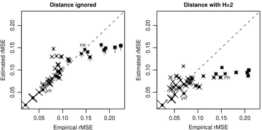
Fig. 2 compares the empirical (simulation-based) and analytical (data-based) estimators of the root-MSEs of the univariate composite estimators with the distance ignored and with distance used with a truncation atH

=

2. The counties

(12)

Fig. 2. The empirical and data-based estimators of the root-MSE of the univariate composite estimators. Filled circles indicate the size of the absolute deviation|θd−θ|, and crosses the population size of the county. The values for counties Priorat and Vallès Oriental are marked by their respective

acronyms, PR and VR.

are represented in both panels by filled circles (

•

) with diameters linearly related to the absolute deviations

|

θ

_d

−

θ

|

and crosses (

×

) of size linearly related to the fourth root of the population sizes. In the left-hand panel, we have two sets of data-based estimators; one estimates each12

θ

dby

σ

ˆ

02(averaging), and the other estimates each12

θ

dby composition. They

are connected by vertical segments and the filled circles are placed at the latter values. County Pla de l’Estany is omitted from both panels; its root-MSEs are grossly underestimated.

The diagram shows that the estimators of the root-MSEs tend to be positively biased for counties with small absolute deviations and negatively biased for counties with large absolute deviations. Estimation of the root-MSE is more precise for more populous counties. Underestimation is substantial for several counties, which have small population sizes and large absolute deviations.

Estimation of the root-MSEs entails much less bias when distance is ignored than when it is taken into account. When the distance is ignored, replacing

(θ

d

−

θ)

2with

σ

02entails no ‘error’ only when

|

θ

d

−

θ

|

=

.

σ

0. Two such counties, Priorat

(PR) and Vallès Oriental (VR), are marked in the diagram. When the distance is ignored, the root-MSEs are estimated with only slight bias, whereas withH

=

2 they are underestimated substantially. In bivariate composition and withH

>

2, the uncertainty is even more pronounced. When the distance is ignored, the root-MSEs are estimated with much greater precision even in bivariate shrinkage. Without Pla de l’Estany, the estimators of the root-MSEs have much smaller biases. Details are omitted.

6.3. Empirical Bayes estimation

Every set of composite estimators has its counterpart set of estimators based on the EB models in which the counties are associated with random effects. Univariate composition corresponds to models with no covariates. The random effects are independent whenH

=

1 (no spatial similarity), and otherwise have the covariance matrix0defined in Section3; they correspond to spatial EBLUP. With the normality assumptions, which admittedly are grossly violated, such models can be fitted by an iterative (Newton–Raphson) algorithm that maximises the corresponding log-likelihood. Conditionally on the regression and the within-county variance, they use the same sufficient statistics as their composition counterparts. We fitted these models for the counterparts of the estimatorsV-Comp-h,V=UorB, andh

=

1

,

2

,

3. The sets of these EB estimators are for a majority of districts, as well as on average, less efficient than their composition counterparts. The average root-MSEs are greater by between 8% and 24%. For the most populous counties, the EB estimators are almost uniformly, although only slightly, less efficient than the composite estimators. In contrast, EB estimators are more efficient for a few sparsely populated counties, but these sets of counties differ from one model to the other.

The MSEs of the estimators are estimated from the conditional variances evaluated in the concluding iteration. They display similar features as the MSEs estimated in the composite estimation: they are approximately unbiased for ‘typical’ counties, overestimate the MSEs for counties with means close to the national mean and underestimate them for the counties with large deviations from the national mean.

6.4. The proportions of single households

The county-level percentages of single-member households are estimated by the same methods as the mean household sizes. The dichotomous nature of the outcome variable entails no additional complexity to the analysis of continuous vari-ables. We found that the root-MSE reductions are in general smaller than for estimating the mean household sizes, but are nevertheless substantial. For bivariate composition, taking into account the distance truncated atH

=

2 yields substan-tial gains. With a truncation atH

=

3, the root-MSE reductions largely cancel out, although the differences between the root-MSEs forH

=

2 andH

=

3 are substantial for a few counties. The comparisons of the MSEs are summarised inTable 3.

(13)

Table 3

Comparisons of the sets of small area estimators of the proportion of single-member households in the counties of Catalonia. The same layout is used as in Table 1.

Direct 0.0200 0.0228 0.0217 0.0243 0.0263 (0.0306) (0.0377) (0.0400) (0.0399) (0.0441) U-Comp-1 0.684 [36] 0.0028 0.0017 0.0043 0.0063 (0.0119) (0.0151) (0.0118) (0.0179) U-Comp-2 0.560 [35] 0.819 [29] −0.0011 0.0015 0.0035 (0.0044) (0.0118) (0.0116) U-Comp-3 0.560 [35] 0.819 [29] 1.001 [19] 0.0026 0.0046 (0.0138) (0.0122) B-Comp-1 0.590 [39] 0.863 [39] 1.054 [15] 1.053 [20] 0.0002 (0.0096) B-Comp-2 0.493 [37] 0.722 [35] 0.882 [31] 0.881 [27] 0.837 [31] 7. Discussion

Composition in small area estimation can be broadly interpreted as a way of exploiting the similarity of the districts. When similarity is related to the distances among the districts the composition can be based on the direct estimators for the rings of the target district. Efficient inference about the extent and pattern of similarity is a key to its successful application. In distinctly non-asymptotic settings, this calls for a parsimonious model for similarity, in which uncertainty about the estimated parameters is more than offset by the improved description of similarity. This balancing act is as important as in the EB estimation. In composite estimation we do not have to associate districts with random effects, nor these effects with a distribution, which are essential elements of the EB analysis.

When distance is ignored, the composite estimators attain greater stability because direct estimators are combined only with the estimator of the overall mean. When distances are used, the basis estimators for some rings ha