Option data and modeling BSM implied
volatility
Matthias R. Fengler
December 2010 Discussion Paper no. 2010-32
Editor: Martina
Flockerzi
University of St. Gallen
Department of Economics
Varnbüelstrasse 19
CH-9000 St. Gallen
Phone +41 71 224 23 25
Fax
+41 71 224 31 35
Email [email protected]
Publisher:
Electronic Publication:
Department of Economics
University of St. Gallen
Varnbüelstrasse 19
CH-9000 St. Gallen
Phone +41 71 224 23 25
Fax
+41 71 224 31 35
http://www.vwa.unisg.ch
Option data and modeling BSM implied
volatility
Matthias R. Fengler
Author’s address:
Matthias R. Fengler, Prof. Dr.
Institute for Mathematics and Statistics
University of St. Gallen
Bodanstrasse 6
CH-9000 St. Gallen
Phone +41 71 224 2457
Fax
+41 71 224 2894
Email [email protected]
Website www. mathstat.unisg.ch
This contribution to the Handbook of Computational Finance, Springer-Verlag, gives an
overview on modeling implied volatility data. After introducing the concept of
Black-Scholes-Merton implied volatility (IV), the empirical stylized facts of IV data are reviewed. We then
discuss recent results on IV surface dynamics and the computational aspects of IV. The main
focus is on various parametric, semi- and nonparametric modeling strategies for IV data,
including ones which respect no-arbitrage bounds.
Keywords
Implied volatility
JEL Classification
Forthcoming: Handbook of Computational Finance, Springer-Verlag
1 Introduction
The discovery of an explicit solution for the valuation of European style call and put options based on the assumption a Geometric Brownian motion driv-ing the underlydriv-ing asset constitutes a landmark in the development of modern financial theory. First published in Black and Scholes (1973), but relying heav-ily on the notion of no-arbitrage in Merton (1973), this solution is nowadays known as the Black-Scholes-Merton (BSM) option pricing formula. In recogni-tion of this achievement, Myron Scholes and Robert C. Merton were awarded the Nobel prize in economics in 1997 (Fischer Black had already died by this time).
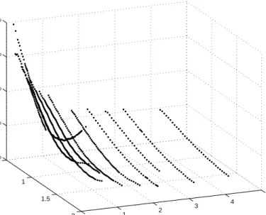
Although it is widely acknowledged that the assumptions underlying the BSM model are far from realistic, the BSM formula still enjoys unrivalled popularity in financial practice. This is not so much because practitioners believe in the model as a good description of market behavior, but rather because it serves as a convenient mapping device from the space of option prices to a single real number called the(BSM-)implied volatility. Indeed, the only unknown parameter involving the BSM formula is the volatility. Backed out of given option prices it allows for straight forward comparisons of the relative expensiveness of options across various strikes, expiries and underlying assets. In practice calls and puts are thus quoted in terms of implied volatility. For illustration consider Figure 1 displaying implied volatility (IV) as ob-served on 28 Oct. 2008 and computed from options traded on the futures exchange EUREX, Frankfurt. IV is plotted against relative strikes and time to expiry. Due to institutional conventions, there is a very limited number of expiry dates, usually one to three months apart for short-dated options and six to twelve months apart for longer-dated ones, while the number of strikes for each expiry is more finely spaced. The function resulting for a fixed expiry is frequently called the ‘IV smile’ due to its U-shaped pattern. For a fixed (relative) strike across several expiries one speaks of the term structure of IV. Understandably, the non-flat surface, which also fluctuates from day to day, is in strong violation to the assumption of a Geometric Brownian motion underlying the BSM model.
Although IV observations are observed on this degenerate design, practi-tioners think of them as stemming from a smooth and well-behaved surface. This view is due to the following objectives in option portfolio management: (i) market makers quote options for strike-expiry pairs which are illiquid or not listed; (ii) pricing engines, which are used to price exotic options and which are based on far more realistic assumptions than the BSM model, are calibrated against an observed IV surface; (iii) the IV surface given by a listed market serves as the market of primary hedging instruments against volatil-ity and gamma risk (second-order sensitivvolatil-ity with respect to the spot); (iv)
0.5 1 1.5 2 0 1 2 3 4 5 20 % 40 % 60 % 80 % 100 %
Time to maturity [years] Moneyness [X/S]
Fig. 1.IV surface of DAX index options from 28 Oct. 2008, traded at the EUREX. IV given in percent across a spot moneyness metric, time to expiry in years.
risk managers use stress scenarios defined on the IV surface to visualize and quantify the risk inherent to option portfolios.
Each of these applications requires suitably chosen interpolation and ex-trapolation techniques or a fully specified model of the IV surface. This sug-gests the following structure of this contribution: Section 2 introduces the BSM-implied volatility and in Section 3 we outline its stylized facts. No-arbitrage constraints on the IV surface are presented in Section 4. In Section 5, recent theoretical advances on the asymptotic behavior of IV are summarized. Approximation formulae and numerical methods to recover IV from quoted option prices are reviewed in Section 6. Parametric, semi- and nonparametric modeling techniques of IV are considered in Section 7.
2 The BSM model and implied volatility
We consider an economy on the time interval [0, T∗]. Let (Ω,F,P) be a prob-ability space equipped with a filtration (Ft)0≤t≤T∗ which is generated by a
Brownian motion (Wt)0≤t≤T∗ defined on this space, see e.g. Steele (2000). A
stock price (St)0≤t≤T∗, adapted to (Ft)0≤t≤T∗ (paying no-dividends for
sim-plicity) is modeled by the Geometric Brownian motion satisfying the stochas-tic differential equation
dSt
St
=µ dt+σ dWt, (1)
whereµdenotes the (constant) instantaneous drift andσ2measures the
(con-stant) instantaneous variance of the return process of (logSt)t≥0. We
further-more assume the existence of a riskless money market account paying interest
r. A European style call is a contingent claim paying at some expiry dateT, 0< T≤T∗, the amountψc(ST) = (ST−X)+, where (·)+ def= max(·,0) andX
is a fixed number, the exercise price. The payoff of a European style put is given byψp(ST) = (X−ST)+.
Under these assumptions, it can be shown that the option price H(St, t)
is a function in the spaceC2,1(R+×(0, T))satisfying the partial differential
equation 0 = ∂H ∂t +rS ∂H ∂S + 1 2σ 2S2∂ 2H ∂S2 −rH (2) subject toH(ST, T) =ψi(ST) withi∈ {c, p}.
The celebrated BSM formula for calls solving (2) with boundary condition
ψc(ST) is found to be CtBSM(X, T) =StΦ(d1)−e−r(T−t)XΦ(d2), (3) with d1= log(St/X) + (r+12σ2)(T−t) σ√T−t , (4) d2=d1−σ √ T−t , (5)
and whereΦ(v) =∫−∞v φ(u)duis the cdf of the standard normal distribution with pdfφ(v) = √1
2πe
−v2/2forv∈R.
Given observed market pricesCet, one defines – as first introduced by
La-tan´e and Rendelman (1976) – implied volatility as b
σ: CtBSM(X, T,σb)−Cet= 0. (6)
Due to monotonicity of the BSM price in σ, there exists a unique solution b
σ∈R+. Note that the definition in (6) is not confined to European options. It is also used for American options, which can be exercised at any time in [0, T]. In this case, as no explicit formulae for American style options exists, the option price is computed numerically, for instance by means of finite difference schemes, Randall and Tavella (2000).
In the BSM model volatility is just a constant, whereas empirically, IV displays a pronounced curvature across strikesX and different expiry daysT. This gives rise to the notion of an IV surface as the mapping
b
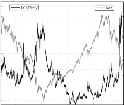
2001 2003 2005 2007 2009 15 % 20 % 25 % 30 % 35 % 40 % 45 % 3000 4000 5000 6000 7000 8000 1Y ATM−IV DAX
Fig. 2. Time series of 1Y ATM IV (left axis, black line) and DAX index closing prices (right axis, gray line) from 2000 to 2008.
In Figure 2, we plot the time series of 1Y at-the-money IV of DAX index options (left axis, black line) together with DAX closing prices (right axis, gray line). An option is called at-the-money (ATM) when the exercise price is equal or close to the spot (or to the forward). The index options were traded at the EUREX, Frankfurt (Germany), from 2000 to 2008. As is visible IV is subject to considerable variations. Average DAX index IV was about 22% with significantly higher levels in times of market stress, such as after the World Trade Center attacks 2001, during the pronounced bear market 2002-2003 and the financial crisis end of 2008.
3 Stylized facts of implied volatility
The IV surface displays a number of static and dynamic stylized facts which we demonstrate here using the present DAX index option data dating from 2000 to 2008. These facts can be observed for any equity index market. They sim-ilarly hold for stocks. Other asset classes may display different features, for instance, smiles may be more shallow, symmetric or even upward-sloping, but
this does not fundamentally change the smile phenomenon. A more complete synthesis can be found in Rebonato (2004).
Stylized facts of IV are as follows:
1. The smile is very pronounced for short expiries and becomes flattish for longer dated options. This fact was already visible in Figure 1.
2. As noted by Rubinstein (1994) this has not always been the case. The strong asymmetry in the smile first appeared after the 1987 market tur-moil.
3. For equity options, both index and stocks, the smile is negatively skewed. We define the ‘skew’ here by ∂∂mbσ2
m=0, wheremis log-forward moneyness
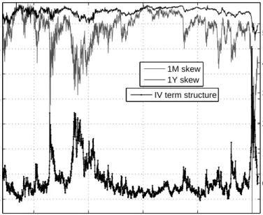
as defined in Section 5. Figure 3 depicts the time series of the DAX index skew (left axis) for 1M and 1Y options. The skew is negative throughout and – particularly the short-term skew – increases during times of crisis. For instance, skews increase in the aftermath of the dot-com boom 2001 to 2003, or spike at 11 Sep. 2001 and during the heights of the financial crisis 2008. As theory predicts, see Section 5, the 1Y IV skew has most of the time been flatter than the 1M IV skew.
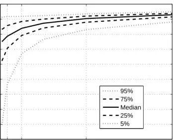
4. Fluctuations of the short-term skew are much larger. Figure 4 gives the quantiles of the skew as a function of time to expiry. Similar patterns also apply to IV levels and returns.
5. The IV surface term structure is typically upward sloping (i.e. has increas-ing levels of IV for longer dated options) in calm times, while in times of crisis it is downward sloping with short dated options having higher levels of IV then longer dated ones. This is seen in Figure 3 giving the differ-ence of 1M ATM IV minus 1Y ATM in terms of percentage points on the right axis. A positive value therefore indicates a downward sloping term structure. During the financial crisis the term structure slope achieved unprecedented levels. Humped profiles can be observed as well.
6. Returns of the underlying asset and returns of IV are negatively correlated. For the present data set we find a correlation between 1M ATM IV and DAX returns ofρ=−0.69.
7. IV appears to be mean-reverting, see Figure 2, but it is usually difficult to confirm mean reversion statistically, since IV data is often found to be nearly integrated, see Fengler et al. (2007) for a discussion.
8. Shocks cross the IV surface are highly correlated, as can be observed from the comovements of IV levels in Figure 2 and the skew and the term structure in Figure 3. In consequence IV surface dynamics can be decomposed into a small number of driving factors, see Chapter ???Set link to Domininik’s Contribution??? of this handbook.
2001 2003 2005 2007 2009 −1.6 −1.4 −1.2 −1 −0.8 −0.6 −0.4 −0.2 Time Skew 0 10 20 30 40 50 IV term structure IV term structure 1M skew 1Y skew
Fig. 3. Time series of 1M and 1Y IV skew (left axis, gray line and black line respectively) and time series of the IV term structure (right axis, black dotted line). Skew is defined as ∂bσ2
∂m
m=0
, wherem is log-forward moneyness. The derivative is approximated by a finite difference quotient. IV term structure is the difference between 1M ATM and 1Y ATM in terms of percentage points. Negative values indicate an upward sloping term structure.
4 Arbitrage bounds on the implied volatility surface
Despite the rich empirical behavior, IV cannot simply assume any functional form. This is due to constraints imposed by no-arbitrage principles. For IV, these constraints are very involved, but are easily stated indirectly in the option price domain. From now on, we sett= 0 and suppress dependence on
t for sake of clarity.
We state the bounds using a (European) call option; deriving the corre-sponding bounds for a put is straightforward. The IV function must be such that the call price is bounded by
max (
S−e−rTX,0 )
≤C(X, T)≤S . (8) Moreover, the call price must be a decreasing and convex function inX, i.e.
−e−rT ≤ ∂C
∂X ≤0 and ∂2C
1M 3M 1Y 2Y −0.9 −0.8 −0.7 −0.6 −0.5 −0.4 −0.3 −0.2 −0.1 0 Time to expiry Skew 95% 75% Median 25% 5%
Fig. 4. Empirical quantiles of the ATM IV skew as a function of time to expiry. Skew is defined as ∂∂mσb2
m=0, wheremis log-forward moneyness.
To preclude calendar arbitrage, prices of American calls for the same strikes must be nondecreasing across increasing expiries. This statement does not hold for European style calls because their theta can change sign. No-arbitrage implies, however, that there exists a monotonicity relationship along forward-moneyness corrected strikes (also in the presence of dividend yield), see Reiner (2000), Gatheral (2004), Kahal´e (2004), Reiner (2004), Fengler (2009). Denote by x = X/FT forward-moneyness, where FT is a forward
with expiry T, and by T1 < T2 the expiry dates of two call options whose
strike pricesX1andX2are related by forward-moneyness, i.e.x1=x2. Then
C(X2, T2)≥C(X1, T1). (10)
Most importantly, this results implies that total implied variance must be non-decreasing in forward-moneyness to preclude arbitrage. Defining total variance as ν2(x, T)def= bσ2(x, T)T, we have
ν2(x, T2)> ν2(x, T1). (11)
Relationship (11) has the important consequence that one can visually check IV smiles for calendar arbitrage by plotting total variance across forward moneyness. If the lines intersect, (11) is violated.
5 Implied volatility surface asymptotics
Many of the following results had the nature of conjectures and were gener-alized and rigorously derived only very recently. Understanding the behavior of IV for far expiries and far strikes is of utter importance for extrapolation problems often arising in practice.
Throughout this section setr= 0 and t= 0. This is without loss of gen-erality since in the presence of nonzero interest rates and dividends yields, the option and underlying asset prices may be viewed as forward prices, see Britten-Jones and Neuberger (2000). Furthermore define log-(forward) mon-eyness bymdef= logx= log(X/S) and total (implied) variance byν2 def= bσ2T.
Let S = (St)t≥0 be a non-negative martingale with S0 > 0 under a fixed
risk-neutral measure.
5.1 Far expiry asymptotics
The results of this section can be found in more detail in Tehranchi (2010) whom we follow closely.
The first theorem shows that the IV surface flattens for infinitely large expiries.
Theorem 1 (Rogers and Tehranchi (2009)). For anyM >0 we have
lim
T→∞m sup
1,m2∈[−M,M]
|bσ(m2, T)−σb(m1, T)|= 0.
Note that this result does not hinge upon the central limit theorem, mean-reversion of spot volatility etc., only the existence of the martingale measure. In particular, limT→∞σb(m, T) does not need to exist for anym.
The rate of flattening of the IV skew can be made more precise by the following result. It shows that the flattening behavior of the IV surface as described in Section 3 is not an empirical artefact, but has a well-founded theoretical underpinning (for earlier, less general arguments see Hodges (1996) and Carr and Wu (2003)).
Theorem 2 (Rogers and Tehranchi (2009)). (i) For any 0≤m1< m2 we have
b
σ(m2, T)2−bσ(m1, T)2
m2−m1 ≤
4
T .
(ii) For anym1< m2≤0
b
σ(m2, T)2−bσ(m1, T)2
m2−m1 ≥ −
4
(iii) IfSt P
−→0 ast→ ∞,for any M >0we have
lim sup T→∞ sup m1, m2∈[−M,M], m1̸=m2 Tσb(m2, T) 2−σb(m 1, T)2 m2−m1 ≤4.
As pointed out by Rogers and Tehranchi (2009), the inequality in (iii) is sharp in the sense that there exists a martingale (St)t≥0withSt
P −→0 such that T ∂ ∂mbσ(m, T) 2→ − 4.
as T → ∞ uniformly for m∈ [−M, M]. The condition St P
−→0 as t → ∞,
is not strong. It holds for most financial models and is equivalent to the statement that
C(X, T) = E[(ST −X)+]→S0
as T → ∞for some X >0. The BSM formula (3) fulfills it trivially. Indeed one can show that if the stock price process does not converge to zero, then limT→∞bσ(m, T) = 0, becauseν2<∞.
Finally Tehranchi (2009) obtains the following representation formula for IV:
Theorem 3 (Tehranchi (2009)). For anyM >0we have
lim T→∞m∈[sup−M, M] bσ(m, T)− √ −8 T log E[ST ∧1]
with a∧b= min(a, b). Moreover there is the representation
b
σ∞2 = lim
T→∞−
8
T log E[ST ∧1] (12)
whenever this limit is finite.
A special case of this result was derived by Lewis (2000) in the context of the Heston (1993) model. For certain model classes, such as models based on L´evy processes, the last theorem allows a direct derivation ofσb∞.
The implication of these results for building an IV surface are far-reaching. The implied variance skew must be bounded by∂ν2
∂m
≤4 and should decay at a rate of 1/T between expiries. Moreover, a constant far expiry extrapolation in σb(m, Tn) beyond the last extant expiry Tn is wrong, since the IV surface
does not flatten in this case. A constant far expiry extrapolation inν2(m, Tn)
beyond Tn is fine, but may not be a very lucky choice given the comments
5.2 Short expiry asymptotics
Roper and Rutkowski (2009) consider the behavior of IV towards small times to expiry. They prove
Theorem 4 (Roper and Rutkowski (2009)). If C(X, ϵ) = (S−X)+ for
someϵ >0 then lim T→0+bσ(X, T) = 0. (13) Otherwise lim T→0+bσ(X, T) = limT→0+ √ 2πC(X,T) S√T ifS=X limT→0+ | log(S/X)| √ −2Tlog[C(X,T)−(S−X)+] ifS̸=X , (14)
in the sense that the LHS is finite (infinite) whenever the RHS is finite (infi-nite).
The quintessence of this theorem is twofold. First, the asymptotic behavior ofbσ(X, T) asT →0+is markedly different forS=X andS ̸=X. Note that
the ATM behavior of (14) is the well-established Brenner and Subrahmanyam (1988)-Feinstein (1988) formula to be presented in Section 6.1. Second, con-vergent IV is not a behavior coming for granted. In particular no-arbitrage does not guarantee that a limit exists, see Roper and Rutkowski (2009) for a lucid example. However, the limit of time-scaled IV exists and is zero:
lim
T→0+ν(X, T) = limT→0+σb √
T = 0. (15)
5.3 Far strike asymptotics
Lee (2004) establishes the behavior of the IV surface as strikes tend to infin-ity. He finds a one-to-one correspondence between the large-strike tail and the number of moments of ST, and the small-strike tail and the number
of moments of ST−1. We retain the martingale assumption for (St)t≥0 and
mdef= log(X/S).
Theorem 5 (Lee (2004)). Define
e
p= sup{p: EST1+p<∞} βR= lim sup m→∞ ν2 |m| = lim supm→∞ b σ2 |m|/T . ThenβR∈[0,2]and e p= 1 2βR +βR 8 − 1 2 ,
with the understanding that1/0 =∞. Equivalently,
βR= 2−4(
√ e
The next theorem considers the casem→ −∞.
Theorem 6 (Lee (2004)). Denote by
e
q= sup{q: EST−q <∞} βL= lim sup m→−∞ ν2 |m| = lim supm→−∞ b σ2 |m|/T . ThenβL∈[0,2]and e q= 1 2βL +βL 8 − 1 2 , with 1/0 =∞, or βL= 2−4( √ e q2+eq−qe).
Roger Lee’s results have again vital implications for the extrapolation of the IV surface for far strikes. They show that linear or convex skews for far strikes are wrong by the O(|m|1/2) behavior. More precisely, the IV wings
should not grow faster than |m|1/2 and not grow slower than |m|1/2, unless
the underlying asset price is supposed to have moments of all orders. The elegant solution following from these results is to extrapolate ν2 linearly in
|m| with an appropriately chosenβL, βR∈[0,2].
6 Approximating and computing implied volatility
6.1 Approximation formulae
There is no closed-form, analytical solution to IV, even for European options. In situations when iterative procedures is not readily available, such as in the context of a spreadsheet, or when numerical approaches are not applicable, such as in real time applications, approximation formulae to IV are of high interest. Furthermore, they also serve as good inital values for the numerical schemes discussed in section 6.2.
The most simple approximation to IV, which is due to Brenner and Sub-rahmanyam (1988) and Feinstein (1988), is given by
b σ≈ √ 2π T C S . (16)
The rationale of this formula can be understood as follows. Define by K def=
S=Xe−rT the discounted ATM strike. The BSM formula then simplifies to
C=S
(
2Φ(σ√T /2)−1 )
.
Solving forσyields the semi-analytical formula
σ= √2 T Φ −1 ( C+S 2S ) , (17)
whereΦ−1denotes the inverse function of the normal cdf. A first order Taylor
expansion of (17) in the neighborhood of1
2yields formula (16). In consequence,
it is exact only, when the spot is equal to the discounted strike price.
A more accurate formula, which also holds for in-the-money (ITM) and out-of- the-money (OTM) options (calls are called OTM when S ≪ X and ITM whenS ≫X), is based on a Taylor expansion of third order toΦ. It is due to Li (2005): b σ≈ 2z √ 2 T − 1 √ T √ 8z2−√6α 2z if ρ≤1.4 1 2√T ( α+ √ α2−4(K−S)2 S(S+K) ) if ρ >1.4, (18) wherez= cos [ 1 3arccos (3α √ 32 )] ,α=S√+2Kπ(2C+K−S) andρ=|K−S|SC−2.
The value of the threshold parameterρseparating the first part, which is for nearly-ATM options, and the second part for deep ITM or OTM options, was found by Li (2005) based on numerical tests.
Other approximation formulae found in the literatur often lack a rigorous mathematical foundation. The possibly most prominent amongst these are those suggested by Corrado and Miller (1996) and Bharadia et al. (1996). The Corrado and Miller (1996) formula is given by
b σ≈√1 T √ 2π S+K C−S−K 2 + √( C−S−K 2 )2 −(S−K)2 π . (19)
Its relative accuracy is explained by the fact that (19) is identical to the second formula in (18) after multiplying the second term under the square root by
1
2(1 +K/S), which is negligible in most cases, see Li (2005) for the details.
Finally, the Bharadia et al. (1996) approximation is given by b σ≈ √ 2π T C−(S−K)/2 S−(S−K)/2 . (20) Isengildina-Massa et al. (2007) investigate the accuracy of six approxi-mation formulae. According to their criteria, Corrado and Miller (1996) is the best approximation followed by Li (2005) and Bharadia et al. (1996). This finding holds uniformly also for deviations to up to 1% around ATM (somewhat unfortunate, the authors do not consider a wider range) and up to maturities of 11 months. As a matter of fact, the approximation by Brenner and Subrahmanyam (1988) and Feinstein (1988) is of competing quality for ATM options only.
6.2 Numerical computation of implied volatility Newton-Raphson
The Newton-Raphson method, which will be the method of first choice in most cases, was suggested by Manaster and Koehler (1982). Denoting the observed market price byCe, the approach is described as
σi+1 =σi− ( Ci(σi)−Ce ) /∂C ∂σ(σi), (21)
where Ci(σi) is the option price and ∂C∂σ(σi) is the option vega computed at
σi. The algorithm is run until a tolerance criterion, such as |Ce−Ci+1| ≤ϵ,
is achieved; IV is given by bσ=σi+1. The algorithm may fail, when the vega
is close to zero, which regularly occurs for (short-dated) far ITM oder OTM options. The Newton-Raphson method has at least quadratic convergence, and combined with a good choice of the initial value, it achieves convergence within a very small number of steps. Originally, Manaster and Koehler (1982) suggested
σ0=
√ 2
T |log(S/X) +rT| (22)
as initial value (setting t = 0). It is likely, however, that the approximation formulae discussed in section 6.1 provide initial values closer to the solution.
Regula falsi
The regula falsi is more robust than Newton-Raphson, but has linear conver-gence only. It is particularly useful when no closed-form expression for the vega is available, or when the price function is kinked as e.g. for American options with high probability of early exercise.
The regula falsi is initialized by two volatility estimatesσL and σH with
corresponding option pricesCL(σL) and CH(σH) which need to include the
solution. The iteration steps are: 1. Compute σi+1=σL− ( CL(σL)−Ce ) σ H−σL CH(σH)−CL(σL) ; (23)
2. if Ci+1(σi+1) and CL(σL) have same sign, set σL = σi+1; if Ci+1(σi+1)
andCH(σH) have same sign, setσH=σi+1. Repeat step 1.
The algorithm is run until|Ce−Ci| ≤ϵ, whereϵthe desired tolerance. Implied
7 Models of implied volatility
7.1 Parametric models of implied volatility
Since it is often very difficult to define a single parametric function for the entire surface (see Chapter 2 in Brockhaus et al. (2000) and Dumas et al. (1998) for suggestions in this directions), a typical approach is to estimate each smile independently by some nonlinear function. The IV surface is then reconstructed by interpolating total variances along forward moneyness as is apparent from section 4. The standard method is linear interpolation. If derivatives of the IV surface with respect to time to expiry are needed, higher order polynomials for interpolation are necessary. Gatheral (2006) suggests the well-behaved cubic interpolation due to Stineman (1980). A monotonic cubic interpolation scheme can be found in Wolberg and Alfy (2002).
In practice a plethora of functional forms is used. The following selection of parametric approaches is driven by their respective popularity in three different asset classes (equity, fixed income, FX markets) and by the solid theoretical underpinnings they are derived from.
Gatheral’s SVI parametrization
The stochastic volatility inspired (SVI) parametrization for the smile was introduced by Gatheral (2004) and is motivated from the asymptotic extreme strikes behavior of a IV smile, which is generated by a Heston (1993) model. It is given in terms of log-forward moneynessm= log(X/F) as
b
σ2(m, T) =a+b
(
ρ(m−c) +√(m−c)2+θ2) , (24)
where a >0 determines the overall level of implied variance andb≥0 (pre-dominantly) the angle between left and right asymptotes of extreme strikes; |ρ| ≤1 rotates the smile around the vertex, andθcontrols the smoothness of the vertex;c translates the graph.
The beauty of Gatheral’s parametrization becomes apparent observing that implied variance behaves linear in the extreme left and right wing as prescribed by the moment formula due to Lee (2004), see section 5.3. It is therefore straight forward to control the wings for no-arbitrage conditions. Indeed, comparing the slopes of the left and right wing asymptotes with The-orem 6, we find that
b(1 +|ρ|)≤ 2
T ,
to preclude arbitrage (asymptotically) in the wings. The SVI appears to fit a wide of range smile patterns, both empirical ones and those of many stochastic volatility and pure jump models, Gatheral (2004).
The SABR parametrization
The SABR parametrization is a truncated expansion of the IV smile which is generated by the SABR model proposed by Hagan et al. (2002). SABR is an acronym for the ‘stochastic αβρmodel’, which is a two-factor stochastic volatility model with parametersα, the initial value of the stochastic volatility factor;β ∈[0,1], an exponent determining the dynamic relationship between the forward and the ATM volatility, where β = 0 gives rise to a ‘stochastic normal’ andβ = 1 to a ‘stochastic log-normal’ behavior;|ρ| ≤1, the correla-tion between the two Brownian mocorrela-tions; andθ >0, the volatility of volatility. The SABR approach is very popular in fixed income markets where each asset only has a single exercise date, such as swaption markets.
Denote byF the forward price,X is as usual the strike price. The SABR parametrization is a second order expansion given by
b σ(X, T) =bσ0(X) { 1 +bσ1(X)T } +O(T2), (25) where the first term is
b σ0(X) = θ χ(z)log F X (26) with z= θ α F1−β−X1−β 1−β and χ(z) = log (√ 1−2ρz+z2+z−ρ 1−ρ ) ; the second term is
b σ1(X) =(1−β) 2 24 α2 (F X)1−β + 1 4 ρβθα (F X)(1−β)/2 + 2−3ρ2 24 θ 2 . (27)
Note that we display here the expansion in the corrected version as was pointed out by Ob l´oj (2008); unlike the original fomula this version behaves consis-tently forβ →1, as thenz(β)→ θ
αlog F X .
The formula (25) is involved, but explicit and can therefore be computed efficiently. For the ATM volatility, i.e.F =X,zandχ(z) disappear, and the first term in (25) collapses to bσ0(F) =αFβ−1.
As a fitting strategy, it is usually recommended to obtainβ from a log-log plot of historical data of the ATM IV bσ(F, F) against F and to exclude it from the subsequent optimizations. Parameterθ andρare inferred from a calibration to observed market IV; during that calibrationαis found implicitly by solving for the (smallest) real root of the resulting cubic polynomial inα, givenθ andρand the ATM IVσb(F, F):
α3(1−β) T 24F2−2β +α 2 ρβθT 4F(1−β) +α 1 + 2−3ρ 24 θ 2T −bσ(F, F)F1−β= 0.
For further details on calibrations issues we refer to Hagan et al. (2002) and West (2005), where the latter has a specific focus on the challenges arising in illiquid markets. Alternatively, Mercurio and Pallavicini (2006) suggest a cali-bration procedure for all parameters (inludingβ) from market data exploiting both swaption smiles and constant maturity swap spreads.
Vanna-Volga method
In terms of input information, the vanna-volga (VV) approach is probably the most parsimonious amongst all constructive methods for building an IV surface, as it relies on as few as three input observations per expiry only. It is popular in FX markets. The VV method is based on the idea of constructing a replication portfolio that is locally risk-free up to second order in spot and volatility in a fictitious setting, where the smile is flat, but varies stochastically over time. Clearly, this setting is not only fictitious, but also theoretically inconsistent, as there is no model which generates a flat smile that fluctuates stochastically. It may however be justified by the market practice of using a BSM model with a regularly updated IV as input factor. The hedging costs incurred by the replication portfolio thus constructed are then added to the flat-smile BSM price.
To fix ideas, denote the option vega by ∂C
∂σ, volga by ∂2C
∂σ2 and vanna by
∂2C
∂σ∂S. We are given three market observations of IVbσi with associated strikes
Xi, i = 1,2,3, with X1 < X2 < X3, and same expiry dates Ti = T for
which the smile is to be constructed. In a first step, the VV method solves the following system of linear equations, for an arbitrary strike X and for some base volatility ˜σ: ∂CBSM ∂σ (X,σ˜) = 3 ∑ i=1 wi(X) ∂CBSM ∂σ (Xi,σ˜) ∂2CBSM ∂σ2 (X,σ˜) = 3 ∑ i=1 wi(X) ∂2CBSM ∂σ2 (Xi,σ˜) (28) ∂2CBSM ∂σ∂S (X,σ˜) = 3 ∑ i=1 wi(X) ∂2CBSM ∂σ∂S (Xi,σ˜)
The system can be solved numerically or analytically for the weightswi(X),
i= 1,2,3. In a second step, the VV price is computed by
C(X) =CBSM(X,˜σ) + 3 ∑ i=1 wi(X) [ CBSM(Xi,bσi)−CBSM(Xi,σ˜) ] , (29)
from which one obtains IV by inverting the BSM formula. These steps need to be solved for eachX to construct the VV smile. For more details on the VV method, approximation formulae for the VV smile, and numerous practical insights we refer to the lucid description presented by Castagna and Mercurio (2007). As a typical choice for the base volatility, Castagna and Mercurio (2007) suggest ˜σ=σ2, whereσ2would be an ATM IV, andσ1andσ3are 25∆
put and the 25∆ call IV, respectively. As noted there, the VV method is not arbitrage-free by construction, in particular convexity can not be guaranteed, but it appears to produce arbitage-free estimates of IV surfaces for usual market conditions.
7.2 Non- and semiparametric models of implied volatility
If potential arbitrage violations in the resulting estimate are of no particular concern, virtually any non- and semiparametric method can be applied to IV data. A specific choice can often be made from practical considerations. We therefore confine this section to pointing to the relevant examples in the literature.
Piecewise quadratic or cubic polynomials to fit single smiles was ap-plied by Shimko (1993), Malz (1997), An´e and Geman (1999) and Hafner and Wallmeier (2001). A¨ıt-Sahalia and Lo (1998), Rosenberg (2000), Cont and da Fonseca (2002) and Fengler et al. (2003) employ a Nadaraya-Watson smoother. Higher order local polynomial smoothing of the IV surface was suggested in Fengler (2005), when the aim is to recover the local volatility function via the Dupire formula, or by H¨ardle et al. (2010) for estimating the empirical pricing kernel. Least-squares kernel regression was suggested in Gouri´eroux et al. (1994) and Fengler and Wang (2009). Audrino and Colangelo (2009) rely on IV surface estimates based on regression trees in a forecasting study. Model selection between fully parametric, semi- and nonparametric specifications is discussed in detail in A¨ıt-Sahalia et al. (2001).
7.3 Implied volatility modeling under no-arbitrage constraints
For certain applications, for instance for local volatility modeling, an arbitrage-free estimate of the IV surface is mandatory. Methods producing arbitrage-arbitrage-free estimates must respect the bounds presented in section 4. They are surveyed in this section.
Call price interpolation
Interpolation techniques to recover a globally arbitrage-free call price function have been suggested by Kahal´e (2004) and Wang et al. (2004). It is crucial for these algorithms to work that the data to be interpolated are arbitrage-free from the beginning. Consider the set of pairs of strikes and call prices
(Xi, Ci), i= 0, . . . , n. Then, applying to (9), the set does not admit arbitrage
in strikes if the first divided differences associated with the data observe −e−rT < Ci−Ci−1
Xi−Xi−1
< Ci+1−Ci Xi+1−Xi
<0 (30)
and if the price bounds (8) hold.
For interpolation Kahal´e (2004) considers piecewise convex polynomials which are inspired from the BSM formula. More precisely, for a parameter vectorΘ= (θ1, θ2, θ3, θ4)⊤ withθ1>0,θ2>0 consider the function
c(X;Θ) =θ1Φ(d1)−X Φ(d2) +θ3X+θ4, (31) where d1 = [ log(θ1/X) + 0.5θ22 ] /θ2 and d2 = d1−θ2. Clearly, c(X;Θ) is
convex in strikes X > 0, since it differs from the BSM formula by a linear term, only. It can be shown that on a segment [Xi, Xi+1] and for Ci, Ci+1
and given first order deratives Ci′ and Ci′+1 there exists a unique vector Θ
interpolating the observed call prices.
Kahal´e (2004) proceeds in showing that for a sequence (Xi, Ci, Ci′) for
i = 0, . . . , n+ 1 with the (limit) conditions X = 0, Xi < Xi+1,Xn+1 =∞,
C0=S0,Cn+1= 0,C0′ =−e−rT andCn′+1= 0 and
Ci′< Ci+1−Ci Xi+1−Xi
< Ci′+1 (32)
for i = 1, . . . , n there exists a unique C1 convex function c(X) described
by a series of vectors Θi for i = 0, . . . , n interpolating observed call prices.
There are 4(n+ 1) parameters inΘi, which are matched by 4nequations in
the interior segments Ci = c(Xi;Θi) and Ci′ = c′(Xi;Θi) for i = 1, . . . , n,
and four additional equations by the four limit conditions in (X0, C0) and
(Xn+1, Cn+1).
A C2 convex function is obtained in the following way: Forj = 1, . . . , n, replace thejth condition on the first order conditions byγj=c′(Xj;Θj) and
γj=c′(Xj;Θj−1), for someγj ∈]lj, lj+1[ andlj= (Cj−Cj−1)/(Xj−Xj−1).
Moreover add the conditionc′′(Xj;Θj) =c′′(Xj;Θj−1). This way the number
of parameters is still equal to the number of constraints.
Concluding, the Kahal´e (2004) algorithm for aC2 call price function is as
follows:
1. Put C0′ =−e−rT,Cn′+1= 0 andCi′= (li+li+1)/2 fori= 1, . . . , n, where
li= (Ci−Ci−1)/(Xi−Xi−1).
2. For each j = 1, . . . , n compute the C1 convex function with continuous second order derivative atXj. ReplaceCj′ =γj.
Kahal´e (2004) suggests to solve the algorithm using the Newton-Raphson method.
An alternative, cubicB-spline interpolation was suggested by Wang et al. (2004). For observed prices (Xi, Ci), i= 0, . . . , n, 0< a=X0 < . . . < Xn =
min ||c′′(X)−e−rTh(X)||22
s.t. c(Xi) =Ci, i= 0, . . . , n , (33)
c′′(X)≥0 X ∈(0,∞),
where||·||2is the (Lebesgue)L2norm on [a, b],hsome prior density (e.g., the
log-normal density) andcthe unknown option price function with absolutely continuous first and second order derivatives on [a, b]. By the Peano kernel theorem, the constraintsc(Xi) =Ci, i= 1, . . . , ncan be replaced by
∫ b a
Bi(X)c′′(X)dX=di, i= 1, . . . , n−2, (34)
where Bi is a normalized linear B-spline with the support on [Xi, Xi+2] and
dithe second divided differences associated with the data. Wang et al. (2004)
show that this infinite-dimensional optimization problem has a unique solution for c′′(X) and how to cast it into a finite-dimensional smooth optimization problem. The resulting function forc(X) is then a cubicB-spline. Finally they devise a generalized Newton method for solving the problem with superlinear convergence.
Call price smoothing by natural cubic splines
For a sample of strikes and call prices, {(Xi, Ci)},Xi∈[a, b] fori= 1, . . . , n,
Fengler (2009) considers the curve estimate defined as minimizer bg of the penalized sum of squares
n ∑ i=1 { Ci−g(Xi) }2 +λ ∫ b a {g′′(v)}2dv . (35) The minimizerbgis a natural cubic spline, and represents a globally arbitrage-free call price function. Smoothness is controlled by the parameter λ > 0. The algorithm suggested by Fengler (2009) observes the no-arbitrage straints (8), (9), and (10). For this purpose the natural cubic spline is con-verted into the value-second derivative representation suggested by Green and Silverman (1994). This allows to formulate a quadratic program solving (35). Putgi=g(ui) andγi =g′′(ui), fori= 1, . . . , n, and defineg= (g1, . . . , gn)⊤
andγ= (γ2, . . . , γn−1)⊤. By definition of a natural cubic spline,γ1=γn= 0.
The natural spline is completely specified by the vectors g and γ, see Sec-tion 2.5 in Green and Silverman (1994) who also suggest the nonstandard notation of the entries inγ.
Sufficient and necessary conditions forg and γto represent a valid cubic spline are formulated via the matrices Q and R. Let hi = ui+1 −ui for
i= 1, . . . , n−1, and define then×(n−2) matrixQby its elementsqi,j, for
i= 1, . . . , nandj= 2, . . . , n−1, given by
qj−1,j =h−j−11, qj,j =−h−j−11−h− 1
forj = 2, . . . , n−1, and qi,j = 0 for|i−j| ≥2, where the columns ofQare
numbered in the same non-standard way as the vectorγ.
The (n−2)×(n−2) matrixRis symmetric and defined by its elements
ri,j fori, j= 2, . . . , n−1, given by
ri,i = 13(hi−1+hi) for i= 2, . . . , n−1
ri,i+1=ri+1,i= 16hi fori= 2, . . . , n−2,
(36) andri,j= 0 for|i−j| ≥2.Ris strictly diagonal dominant, and thus strictly
positive-definite.
Arbitrage-free smoothing of the call price surface can be cast into the following iterative quadratic minimization problem. Define a (2n−2)-vector
y= (y1, . . . , yn,0, . . . ,0)⊤, a (2n−2)-vectorξ= (g⊤, γ⊤)⊤ and the matrices,
A=(Q,−R⊤)and B= ( In 0 0 λR ) , (37)
whereIn is the unit matrix with sizen. Then
1. Estimate the IV surface by means of an initial estimate on a regular forward-moneyness gridJ = [x1, xn]×[T1, Tm].
2. Iterate through the price surface from the last to the first expiry, and solve the following quadratic programs.
ForTj, j=m, . . . ,1, solve min ξ −y ⊤ξ+1 2ξ ⊤Bξ (38) subject to A⊤ξ= 0 γi≥0 g2−g1 h1 − h1 6γ2≥ −e− rTj −gn−gn−1 hn−1 − hn−1 6 γn−1≥0 g1≤St if j=m g(ij)< gi(j+1) if j∈[m−1,1] for i= 1, . . . , n (∗) g1≥St−e−rTju1 gn≥0 (39)
whereξ = (g⊤, γ⊤)⊤. Note that we suppress the explicit dependence on
j except in conditions (∗) to keep the notation more readable. Condi-tions (∗) implement (10); thereforegi(j)andgi(j+1)are related by forward-moneyness.
The resulting price surface is converted into IV. It can be beneficial obtain a first coarse estimate of the surface by gridding it on the estimation grid. This allows to more easily implement condition (10). The minimization prob-lem can be solved by using the quadratic programming devices provided by standard statistical software packages. The reader is referred to Fengler (2009) for the computational details and the choice of the smoothing parameterλ. In contrast to the approach by Kahal´e (2004), a potential drawback this ap-proach suffers from is the fact that the call price function is approximated by cubic polynomials. This can turn out to be disadvantageous, since the pricing function is not in the domain of polynomials functions. It is remedied however by the choice of a sufficiently dense grid in the strike dimension inJ.
IV smoothing using local polynomials
As an alternative to smoothing in the call price domain Benko et al. (2007) suggest to directly smooth IV by means of constrained local quadratic polyno-mials. This implies minimization of the following (local) least squares criterion
min α0,α1,α2 n ∑ i=1 { e σi−α0−α1(xi−x)−α2(xi−x)2 }2 Kh(x−xi), (40)
where eσ is observed IV. We denote by Kh(x−xi) = h−1K
(x−xi
h
)
and by K a kernel function – typically a symmetric density function with compact support, e.g. K(u) = 34(1−u2)1(|u| ≤ 1), the Epanechnikov kernel, where
1(A) is the indicator function of some set A. Finally, h is the bandwidth which governs the trade-off between bias and variance, see H¨ardle (1990) for the details on nonparametric regression. Since Kh is nonnegative within the
(localization) window [x−h, x+h], points outside of this interval do not have any influence on the estimatorbσ(x).
No-arbitrage conditions in terms of IV are obtained by computing (9) for an IV adjusted BSM formula, see Brunner and Hafner (2003) among oth-ers. Expressed in forward moneyness x=X/F this yields for the convexity condition ∂2CBSM ∂x2 =e− rT√T φ(d 1) × { 1 x2bσT + 2d1 xbσ√T ∂bσ ∂x + d1d2 b σ ( ∂σb ∂x )2 +∂ 2bσ ∂x2 } (41)
whered1 andd2are defined as in (4) and (5).
The key property of local polynomial regression is that it yields simultane-ously to the regression function its derivatives. More precisely, comparing (40) with the Taylor expansion ofσbshows that
b
Based on this fact Benko et al. (2007) suggest to miminize (40) subject to e−rT√T φ(d1) { 1 x2α 0T + 2d1α1 xα0 √ T + d1d2 α0 (α1) 2 + 2α2 } ≥0, (43) with d1= α2 0T /2−log(x) σ√T , d2=d1−α0 √ T .
This leads to a nonlinear optimization problem inα0, α1, α2.
The case of the entire IV surface is more involved. Suppose the purpose is to estimate σb(x, T) for a set of maturities {T1, . . . , TL}. By (11), for a
given value x, we need to ensure bν2(x, T
l,) ≤ νb2(x, Tl′), for all Tl < Tl′.
Denote by Khx,hT(x−xi, Tl−Ti) a bivariate kernel function given by the
product of the two univariate kernel functionsKhx(x−xi) andKhT(T−Ti).
Extending (40) linearly into the time-to-maturiy dimension then leads to the following optimization problem:
min α(l) L ∑ l=1 n ∑ i=1 Khx,hT(x−xi, Tl−Ti) { e σi−α0(l) −α1(l)(xi−x)−α2(l)(Ti−T)−α1,1(l)(xi−x)2 −α1,2(l)(xi−x)(Ti−T) }2 (44) subject to √ Tlφ(d1(l)) { 1 x2α 0(l)Tl +2d1(l)α1(l) xα0(l) √ Tl +d1(l)d2(l) a0(l) α21(l) + 2α1,1(l) } ≥ 0, d1(l) = α02(l)Tl/2−log(x) α0(l) √ Tl , d2(l) =d1(l)−a0(l) √ Tl, l= 1, . . . , L 2Tlα0(l)α2(l) +α20(l)>0 l= 1, . . . , L α20(l)Tl< α20(l′)Tl′, Tl < Tl′ .
The last two conditions ensure that total implied variance is (locally) nonde-creasing, since ∂ν∂T2 >0 can be rewritten as 2T α0α2+α20 >0 for a given T,
while the last conditions guarantee that total variance is increasing across the surface. From a computational view, problem (44) calculates for a givenxthe estimates for all givenTl in one step in order to warrant thatbν is increasing
in T.
The approach by Benko et al. (2007) yields an IV surface that respects the convexity conditions, but neglects the conditions on call spreads and the general price bounds. Therefore the surface may not be fully arbitrage-free. However, since convexity violations and calendar arbitrage are by far the most virulent instances of arbitrage in observed IV data occurring the surfaces will be acceptable in most cases.
References
A¨ıt-Sahalia, Y., Bickel, P. J. and Stoker, T. M. (2001). Goodness-of-fit tests for regression using kernel methods,Journal of Econometrics105: 363–412. A¨ıt-Sahalia, Y. and Lo, A. (1998). Nonparametric estimation of state-price densities implicit in financial asset prices,Journal of Finance53: 499–548. An´e, T. and Geman, H. (1999). Stochastic volatility and transaction time:
An activity-based volatility estimator,Journal of Risk2(1): 57–69. Audrino, F. and Colangelo, D. (2009). Semi-parametric forecasts of the
im-plied volatility surface using regression trees, Statistics and Computing . Forthcoming.
Benko, M., Fengler, M. R., H¨ardle, W. and Kopa, M. (2007). On extracting information implied in options,Computational Statistics 22(4): 543–553. Bharadia, M. A., Christofides, N. and Salkin, G. R. (1996). Computing the
Black-Scholes implied volatility - generalization of a simple formula,inP. P. Boyle, F. A. Longstaff, P. Ritchken, D. M. Chance and R. R. Trippi (eds),
Advances in Futures and Options Research, Vol. 8, JAI Press, London, pp. 15–29.
Black, F. and Scholes, M. (1973). The pricing of options and corporate liabil-ities,Journal of Political Economy81: 637–654.
Brenner, M. and Subrahmanyam, M. (1988). A simple formula to compute the implied standard deviation,Financial Analysts Journal44(5): 80–83. Britten-Jones, M. and Neuberger, A. J. (2000). Option prices, implied price
processes, and stochastic volatility,Journal of Finance55(2): 839–866. Brockhaus, O., Farkas, M., Ferraris, A., Long, D. and Overhaus, M. (2000).
Equity derivatives and market risk models, Risk Books, London.
Brunner, B. and Hafner, R. (2003). Arbitrage-free estimation of the risk-neutral density from the implied volatility smile,Journal of Computational Finance7(1): 75–106.
Carr, P. and Wu, L. (2003). Finite moment log stable process and option pricing,Journal of Finance58(2): 753–777.
Castagna, A. and Mercurio, F. (2007). Building implied volatility surfaces from the available market quotes: a unified approach, in I. Nelken (ed.),
Volatility as an asset class, Risk Books, Haymarket, London, pp. 3–59. Cont, R. and da Fonseca, J. (2002). The dynamics of implied volatility
sur-faces,Quantitative Finance 2(1): 45–60.
Corrado, C. J. and Miller, T. W. (1996). A note on a simple, accurate formula to compute implied standard deviations, Journal of Banking and Finance 20: 595–603.
Dumas, B., Fleming, J. and Whaley, R. E. (1998). Implied volatility functions: Empirical tests,Journal of Finance53(6): 2059–2106.
Feinstein, S. (1988). A source of unbiased implied volatility,Technical Report 88-9, Federal Reserve Bank of Atlanta.
Fengler, M. R. (2005).Semiparametric Modeling of Implied Volatility, Lecture Notes in Finance, Springer-Verlag, Berlin, Heidelberg.
Fengler, M. R. (2009). Arbitrage-free smoothing of the implied volatility surface,Quantitative Finance9(4): 417–428.
Fengler, M. R., H¨ardle, W. and Mammen, E. (2007). A semiparametric factor model for implied volatility surface dynamics,Journal of Financial Econo-metrics5(2): 189–218.
Fengler, M. R., H¨ardle, W. and Villa, C. (2003). The dynamics of implied volatilities: A common principle components approach, Review of Deriva-tives Research6: 179–202.
Fengler, M. R. and Wang, Q. (2009). Least squares kernel smoothing of the implied volatility smile,inW. H¨ardle, N. Hautsch and L. Overbeck (eds),
Applied Quantitative Finance, 2nd edn, Springer-Verlag, Berlin, Heidelberg. Gatheral, J. (2004). A parsimonious arbitrage-free implied volatility param-eterization with application to the valuation of volatility derivatives, Pre-sentation at the ICBI Global Derivatives and Risk Management, Madrid, Espa˜na.
Gatheral, J. (2006). The Volatility Surface: A Practitioner’s Guide, John Wiley & Sons, Hoboken, New Jersey.
Gouri´eroux, C., Monfort, A. and Tenreiro, C. (1994). Nonparametric diag-nostics for structural models,Document de travail 9405, CREST, Paris. Green, P. J. and Silverman, B. W. (1994). Nonparametric regression and
generalized linear models, Vol. 58 ofMonographs on Statistics and Applied Probability, Chapman and Hall, London.
Hafner, R. and Wallmeier, M. (2001). The dynamics of DAX implied volatil-ities,International Quarterly Journal of Finance1(1): 1–27.
Hagan, P., Kumar, D., Lesniewski, A. and Woodward, D. (2002). Managing smile risk,Wilmott Magazine1: 84–108.
H¨ardle, W. (1990). Applied Nonparametric Regression, Cambridge University Press, Cambridge, UK.
H¨ardle, W., Okhrin, O. and Wang, W. (2010). Uniform confidence bands for pricing kernels,SFB 649 Discussion Paper 2010-03, Humboldt-Universit¨at zu Berlin, Berlin.
Heston, S. (1993). A closed-form solution for options with stochastic volatility with applications to bond and currency options,Review of Financial Studies 6: 327–343.
Hodges, H. M. (1996). Arbitrage bounds on the implied volatility strike and term structures of European-style options,Journal of Derivatives3: 23–35. Isengildina-Massa, O., Curtis, C., Bridges, W. and Nian, M. (2007). Accuracy of implied volatility approximations using “nearest-to-the-money” option premiums,Technical report, Southern Agricultural Economics Association. Kahal´e, N. (2004). An arbitrage-free interpolation of volatilities, RISK
17(5): 102–106.
Latan´e, H. A. and Rendelman, J. (1976). Standard deviations of stock price ratios implied in option prices,Journal of Finance 31: 369–381.
Lee, R. W. (2004). The moment formula for implied volatility at extreme strikes,Mathematical Finance14(3): 469–480.
Li, S. (2005). A new formula for computing implied volatility,Applied Math-ematics and Computation170(1): 611–625.
Malz, A. M. (1997). Estimating the probability distribution of the future exchange rate from option prices,Journal of Derivatives5(2): 18–36. Manaster, S. and Koehler, G. (1982). The calculation of implied variances
from the Black-and-Scholes model: A note, Journal of Finance 37: 227– 230.
Mercurio, F. and Pallavicini, A. (2006). Smiling at convexity: bridging swap-tion skews and CMS adjustments,RISK19(8): 64–69.
Merton, R. C. (1973). Theory of rational option pricing, Bell Journal of Economics and Management Science4(Spring): 141–183.
Ob l´oj, J. (2008). Fine-tune your smile: Correction to hagan et al., Wilmott MagazineMay.
Randall, C. and Tavella, D. (2000).Pricing Financial Instruments: The Finite Difference Method, John Wiley & Sons, New York.
Rebonato, R. (2004). Volatility and Correlation, Wiley Series in Financial Engineering, 2nd. edn, John Wiley & Son Ltd.
Reiner, E. (2000). Calendar spreads, characteristic functions, and variance interpolation. Mimeo.
Reiner, E. (2004). The characteristic curve approach to arbitrage-free time interpolation of volatility, presentation at the ICBI Global Derivatives and Risk Management, Madrid, Espa˜na.
Rogers, L. C. G. and Tehranchi, M. (2009). Can the implied volatility surface move by parallel shifts?,Finance and Stochastics . Forthcoming.
Roper, M. and Rutkowski, M. (2009). On the relationship between the call price surface and the implied volatility surface close to expiry,International Journal of Theoretical and Applied Finance12(4): 427–441.
Rosenberg, J. (2000). Implied volatility functions: A reprise, Journal of Derivatives7: 51–64.
Rubinstein, M. (1994). Implied binomial trees, Journal of Finance 49: 771– 818.
Shimko, D. (1993). Bounds on probability,RISK6(4): 33–37.
Steele, J. M. (2000).Stochastic Calculus and Financial Applications, Springer-Verlag, Berlin, Heidelberg, New York.
Stineman, R. W. (1980). A consistently well-behaved method of interpolation,
Creative Computing6(7): 54–57.
Tehranchi, M. (2009). Asymptotics of implied volatility far from maturity,
Journal of Applied Probability46(3): 629–650.
Tehranchi, M. (2010). Implied volatility: long maturity behavior,inR. Cont (ed.), Encyclopedia of Quantitative Finance, John Wiley & Sons. Forth-coming.
Wang, Y., Yin., H. and Qi, L. (2004). No-arbitrage interpolation of the option price function and its reformulation, Journal of Optimization Theory and Applications120(3): 627–649.
West, G. (2005). Calibration of the SABR model in illiquid markets,Applied Mathematical Finance12(4): 371–385.
Wolberg, G. and Alfy, I. (2002). An energy-minimization framework for monotonic cubic spline interpolation, Journal of Computational and Ap-plied Mathematics143: 145–188.