Accounting for Complex Sample Designs in Multiple Imputation Using the Finite Population Bayesian Bootstrap.

(1)

Accounting for Complex Sample Designs in Multiple Imputation Using the Finite Population Bayesian Bootstrap

By Hanzhi Zhou

A dissertation submitted in partial fulfillment of the requirements for the degree of

Doctor of Philosophy (Survey Methodology) in The University of Michigan

2014

Doctoral Committee:

Professor Michael R. Elliott, Co-Chair

Professor Trivellore E. Raghunathan, Co-Chair Professor Roderick J. Little

Assistant Professor Brady T. West

(2)

© Hanzhi Zhou 2014

(3)

ii

DEDICATION

(4)

iii

ACKNOWLEDGEMENTS

My utmost gratitude goes to my advisors, Mike Elliott and Trivellore Raghunathan, who have been incredibly supportive during my doctoral study. Without Mike and Raghu, I would have had a hard time developing from a student to a researcher. They should also be credited for inspiring this dissertation topic and providing regular guidance throughout this research. I would especially like to thank Mike for the late hours he has spent reviewing my dissertation as we approached the date of my defense.

Special thanks to my dissertation committee members: Rod Little, Rick Valliant and Brady West. I am grateful to Rod, whose constructive comments on my research and whose own tremendous work helped me understand everything better. I am also indebted to Rick and Brady, who carefully read many drafts of my writing and provided useful feedback throughout the development of this research.

Further thanks to faculty members in the Program in Survey Methodology (PSM): Jim Lepkowski, Steve Heeringa, Fred Conrad and Mick Couper, for providing me with interesting teaching and research assistantships over the years.

Lastly but most importantly, I would like to thank my wonderful family: my parents and my brother, their wisdoms, support and love accompanied me along the journey. I would also like to thank my terrific husband and my very best friend, Guihua,

(5)

iv

who understood and shared every bit of my disappointments and successes through the past 10 years.

(6)

v

LIST OF FIGURES

Figure 1.1 The data from a sample survey in the absence of missing data ... 3

Figure 1.2 The data from a sample survey with item nonresponse on the outcome ... 6

Figure 2.1 The procedure to create a single imputed synthetic dataset ... 25

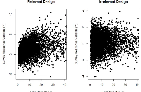
Figure 2.2 Scatter plots of survey variable Y versus size variable Z. ... 37

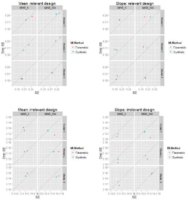
Figure 2.3 Scatter plots of 100 estimated standard errors (SEs) of the mean ... 47

Figure 2.4 Plots of standard error (SE) versus empirical standard error (Emp.SE)... 48

Figure 4.1 Correlation among variables in the simulated population ... 126

Figure 4.2 Distribution of weights under the two subsampling schemes ... 127

Figure 4.3 Comparison of point and interval estimation for 19 population quantiles using the Stratified Boot-FPBB and the design-based complete data analysis for subsampling scheme1. ... 134

Figure 4.4 Comparison of point and interval estimation for 19 population quantiles using the Stratified Boot-FPBB and the design-based complete data analysis for subsampling scheme2. ... 134

Figure 4.5 Comparison of point and interval estimation for 19 population quantiles using the stratified double weighted-FPBB and the design-based complete data analysis for subsampling scheme1. ... 135

Figure 4.6 Comparison of point and interval estimation for 19 population quantiles using the stratified double weighted-FPBB and the design-based complete data analysis for subsampling scheme2. ... 135

(10)

ix

LIST OF TABLES

Table 2.1 Strength of association of the sampling weight with both missingness and outcome variable ... 36 Table 2.2 Before deletion study of the effects of the number of generated FPBB

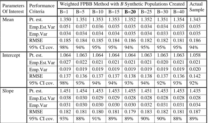
populations (B) on variance estimate ... 44 Table 2.3 Performance of the proposed method in contrast to the fully parametric method

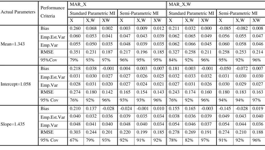
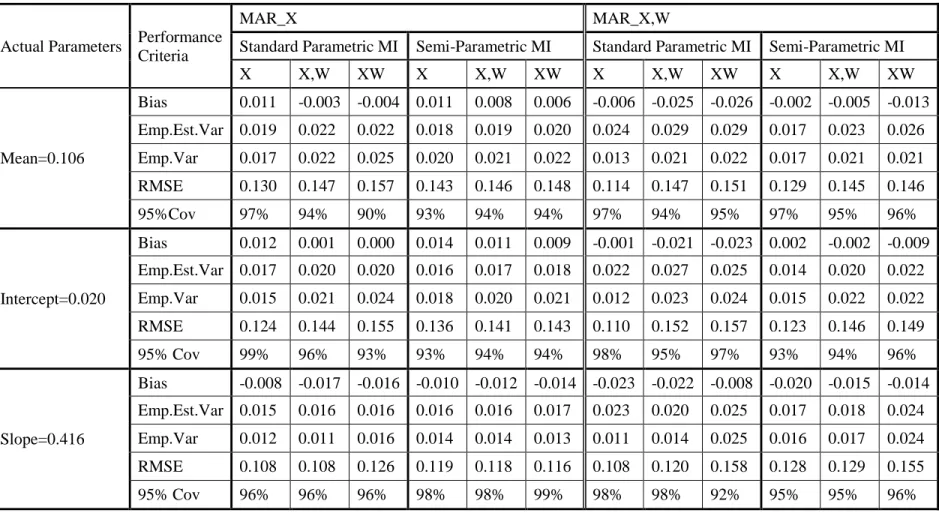
under the relevant design condition ... 45 Table 2.4 Performance of the proposed method in contrast to the fully parametric method

under the irrelevant design condition ... 46 Table 2.5 Estimation of marginal distributions for income and health insurance, and linear

regression coefficients for the regression of BMI on income, age and gender ... 53 Table 2.6 Estimation of log-linear model for four categorical variables (collapse

categories for medium and high income) ... 54 Table 2.7 Estimation of general location model for joint distribution of BMI, age, income

and gender after MI under alternative methods ... 55 Table 3.1 Performance of alternative MI methods for estimating the Mean: population 1,

unbalanced two-stage sample design ... 88 Table 3.2 Performance of alternative MI methods for the Slope: population 1, unbalanced

two-stage sample design ... 89 Table 3.3 Performance of alternative methods for estimating the mean: ... 93 Table 3.4 Performance of alternative methods for estimating the slope: ... 93 Table 3.5 Performance of alternative MI methods for estimating the mean: population

structure 2, unbalanced two-stage sampling design. ... 94 Table 3.6 Performance of alternative MI methods for estimating the slope: population

structure 2, unbalanced two-stage sampling design. ... 96 Table 3.7 Summary of selected survey variables for imputation ... 99 Table 3.8 Estimating mean Delta-V, odds ratio of severe injury given Delta-V, and odds

(11)

x

ratio of head injury given Delta-V... 101 Table 4.1 Comparison of average width 102and 95% CI coverage rates of q( ) for

0.05, 0.10, 0.25, 0.50, 0.75, 0.90 and 0.95.

  ... 136 Table 4.2 Comparison of RelBias, RMSE and 95% CI coverage rates for the mean of Y1

and proportions of Y3 and Y4, ... 137 Table 4.3 Comparison of RelBias, RMSE and 95% CI coverage rates for the regression

coefficients of Y1, Y3 and Y4 on Y2, ... 138 Table 4.4 Alternative methods in estimating the median of BMI and the health insurance

(12)

xi

ABSTRACT

Multiple imputation (MI) is a well-established method to handle

item-nonresponse in sample surveys. Survey data obtained from complex sampling designs often involve features that include unequal probability of selection, clustering and stratification. Because sample design features are frequently related to survey outcomes of interest, the theory of MI requires including them in the imputation model to reduce the risks of model misspecification and hence to avoid biased inference. However, in practice multiply-imputed datasets from complex sample designs are typically imputed under simple random sampling assumptions and then analyzed using methods that account for the design features. Less commonly-used alternatives such as including case weights and/or dummy variables for strata and clusters as predictors typically require interaction terms for more complex estimators such as regression coefficients, and can be vulnerable to model misspecification and difficult to implement.

We develop a simple two-step MI framework that accounts for complex sample designs using a weighted finite population Bayesian bootstrap (FPBB) method to generate draws from the posterior predictive distribution of the population. Imputations may then be performed assuming IID data. We propose different variations of the weighted FPBB for different sampling designs, and evaluate these methods using three studies. Simulation results show that the proposed methods have good frequentist properties and are robust to model misspecification compared to alternative approaches. We apply the proposed method to accommodate missing data in the Behavioral Risk Factor Surveillance System, the National Automotive Sampling System and the National

(13)

xii

Health and Nutrition Examination Survey III when estimating means, quantiles and a variety of model parameters.

(14)

1

CHAPTER 1 INTRODUCTION 1.1 Objectives

Probability sample surveys where each member of the population has a known, non-zero probability of being selected form the backbone of empirical research in social science and public health. To assure broad representativeness, many sample survey designs use unequal probabilities of selection, selection of subjects in stages (introducing clustering) and stratification (For theoretical accounts of sampling methods, see Cochran, 1977 and Särndal et al., 1992). Accordingly, analysis methods for survey data need to take into account these complex sample design features.

It is notable that even the most well-designed sample surveys are imperfect in various ways. Missing data presents a particular challenge. Unit nonresponse occurs when sampled individuals fail to participate in the survey at all. Item nonresponse occurs when sampled individuals do not respond to certain questions. This is common in large scale surveys that include an extensive collection of questions. One principled approach to handle item nonresponse is multiple imputation (MI) (Rubin 1987). The key to success with MI lies in specifying an imputation model that reasonably describes the conditional distribution of the missing data given the observed data. Since complex sample design features frequently are related to survey variables, it is important to include them in the imputation model to reduce the risks of model misspecification and hence to avoid biased inference (Reiter, Raghunathan & Kinney, 2006). This thesis concerns methods that use

(15)

2

MI to deal with item nonresponse while accounting for complex sample designs. It has two objectives:

(1) To illustrate the bias that can arise using existing MI methods to account for complex sample designs when the imputation model is misspecified;

(2) To propose and evaluate a modified MI framework that accounts for complex sample designs with simpler modeling and with no resort to design-based estimators.

We explore the impact of the interrelationship among the data, the sampling mechanism and the missingness mechanism on the performances of the existing and the proposed MI methods. We use both simulated data and real survey data. The following assumptions are made throughout the thesis:

(1) There are no unit nonresponse problems; (2) The data are missing at random (MAR).

Section 1.2 reviews approaches to survey sampling inference in the complete data context, with a focus on Bayesian approach. Section 1.3 reviews the standard multiple imputation (MI) as a well-established method to handle item nonresponse that has a Bayesian justification. The importance of accounting for complex sample designs in MI is discussed from a theoretical perspective. Section 1.4 and 1.5 point out the limitations of current techniques, and introduce the proposed method that builds upon the method reviewed in section 1.2. Finally, section 1.6 outlines the research question each chapter addresses.

(16)

3

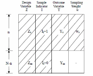
Consider a finite population of size N with two types of measurement on the population units: { ,Y Z_i _i} for i1,...,N, where Y represents a single survey outcome of interest, and Z represents the design variable used for sample selection. We consider three types of Z in this thesis: (1) size measure for probability-proportional-to-size (PPS) sampling, (2) cluster indicators for two-stage cluster sampling, and (3) stratum indicators for stratified sample design. Typically Z is known for all units of the population to the sampler, but not necessarily to the data analyst. Let I_i { ,...,I₁ I_N} denote the vector of sample indicator variables, such that I_i 1 if unit i is sampled and 0 otherwise. We use subscripts s and ns to denote the selected sample of size n and the nonsampled part of the population of size N-n, respectively. Thus both Y and Z divide into two parts:

{( ,Y Y_s _ns), (Z Z_s, _ns)}. Let w_s { ,w i_i 1,..., .}n denote the sampling weights, e.g.

1

1/ N /

i i _i i i

w   



_ Z nZ for a single-stage PPS sampling design. Figure 1.1 illustrates the data from a sample survey in the absence of missing data.

(17)

4

In survey sampling, the objective is usually to learn about some population quantity denoted by Q Y( ), e.g. population mean/quantile/total, etc.,through relating Y_s to Y_nsin some fashion. There are two general inferential frameworks to accomplish this: 1) the design-based approach (Hansen, Hurwitz & Madow, 1953; Cochran, 1977) treats the survey outcome Y as a fixed quantity, and imposes a random distribution on the sample inclusion indicator I. The statistical distribution of an estimator for Q Y( ) is thus induced by the sampling design. While the design-based framework brings in an objectivity element by minimizing the use of modeling assumptions, this objectivity is lost in the presence of nonsampling errors like nonresponse; 2) the model-based approaches, which include the frequentist modeling (Royall, 1970; Valliant et al., 2000) and the Bayesian modeling (Ericson, 1969; Basu, 1971). These regard the survey outcome Y as a random variable as well as I, and assume a model to predict Yns from Ys. Both variants assume

that Y comes from some parametric family of distributions indexed by the parameter . While the frequentist modeling treats  as fixed, and bases inferences on repeated sampling from the model, the Bayesian modeling specifies a prior distribution on  in

addition to Y. The posterior distribution of  given the observed sample ( |p Y_s), and hence the posterior predictive distribution of the nonsampled population values given the

sampled data (p Y_ns|Y_s)



p Y( _ns| , ) ( | Y p_s  Y d_s) , serves as the basis for inference about ( )

Q Y .

The Bayesian paradigm provides the most satisfying inferential approach to survey inference when it is done right. That is by incorporating complex sample design features to avoid sensitivity to model misspecification, using noninformative priors to

(18)

5

avoid subjectivity, and being frequentist calibrated, i.e. having good repeated sampling properties (Little, 2004; Little & Zheng, 2007). Bayesian finite population inference is thus proposed as a means to harmonize design- and model-based approaches for sample survey inference (Little, 2006, 2011; Gelman, 2007), and is exemplified by a variety of work in the complete data context. When design variables or the selection probabilities are known for all units in the population, Zheng and Little (2003, 2005) and Chen, Elliott and Little (2010) propose robust Bayesian predictive inference that improves efficiency over design-based estimators, using penalized splines under fairly weak model

assumptions. In situations where the sizes of the non-sampled units are unavailable, Little and Zheng (2007) and Sangeneh, Keener and Little (2011) consider a two-step procedure to assure ignorable sampling (Sugden and Smith, 1984) with a PPS sampling design. In the first step, the nonsampled sizes (Zns) are predicted by a modified Bayesian Bootstrap

(BB) procedure that adjusts for unequal probability sample selection (ws), i.e.

( _ns | _s, _s)

p Z Z w ; the nonsampled survey outcomes (Ys) are then predicted using a penalized

spline model relating Y with Z, i.e. (p Yns|Y Zs, ).

The modified BB considered by Little and Zheng (2007) is a noninformative Bayesian method closely related to an offshoot of the Bayesian approach to surveys, known as the “Pseudo-Bayesian approach” (Ghosh & Meeden, 1997; Cohen, 1997; Dong,

Elliott & Raghunathan, 2014). The modified BB is of particular interest in this thesis. Details of how our proposed methodology in this thesis builds upon and compares with these methods will be discussed in section 1.5 and in later chapters.

1.3 Standard multiple imputation as a calibrated Bayesian method to deal with item nonresponse

(19)

6

Consider the same finite population as in section 1.2, and assume item

nonresponse occurs on the outcome variable Y and a covariate X is completely observed. Let R_i { ,...,R₁ R_N} denote the response indicator variable for Y, such that R_i 1 if unit i provides a value for Y and 0 otherwise. Write R(R R_s, _ns), where R_s is observable from the sample and R_nsis unobservable for the nonsampled population. We use subscripts obs and mis to denote the responding and the non-responding units, respectively. Thus Ys

further breaks down to Ys,obs and Ys,mis, and Y (Ys obs, ,Ynobs) if we recombine Ys mis, with

ns

Y as unobserved data Y_nobs. The observed data may be thought as the outcome of two random processes: sampling and responding. We illustrate in Figure 1.2 the data from a sample survey with item nonresponse occurring on the survey outcome. Three types of population quantities are of interest in the thesis: the mean/proportion of Y, the regression coefficients of Y on X, and the quantiles of a continuous outcome Y.

Figure 1.2 The data from a sample survey with item nonresponse on the outcome variable

The Bayesian modeling paradigm deals with nonresponse naturally, since unknowns about the finite population given the observed data can be generated from a

(20)

7

predictive distribution. We thus consider multiple imputation (MI) to deal with item nonresponse which has a Bayesian justification. The basic idea of MI is to replace each missing value with a set of plausible values which can then be combined in a simple way for inference using compete-data analysis techniques. The fundamental conceptualization of MI is Bayesian, where the posterior distribution of the model parameters  of interest is obtained by averaging the completed data posterior of  over the posterior predictive distribution of the missing data (Rubin, 1987, Result 3.1):

, , , ,

( | _{s obs}, _s, , _s, ) ( | _s, _s, , _s, ) ( _{s mis}| _{s obs}, _s, , _s, ) _{s mis}

p Y X Z R I 





p( | Y X Z p Ys, s, ) ( s mis, |Ys obs, ,X Z dYs, ) s mis, , allowing the sampling and response mechanism to be ignored in the modeling.

This integration is typically accomplished using Markov Chain Monte Carlo data augmentation (Tanner & Wong, 1987). Let t index the iteration. Draws from the posterior predictive distribution of the missing data ( ( ), | , , , )

t

s mis s obs s

p Y Y X Z are obtained by iterating between draws of the model parameters conditional on the “filled in data”

( ) ( 1)

, ,

( t | _{s obs}, _{s mis}t ,, _s, )

p Y Y  X Z and imputations of the missing data conditional on the observed data and draw of the model parameter p Y( _{s mis}( )_,t |Y_{s obs}_, ,( )t ,X Z_s, ). Rubin (1987) develops simple combining rules to obtain estimates of posterior means and variances using only a finite number (M) of independent draws



(1), ,..., (, )



M s mis s mis

Y Y of the imputed data together with ,

s obs

Y , i.e. multiple “completed” datasets y_comp( )l 



(Y_{s obs}_, ,Y_{s mis}( )_,l ),l1,...,M



. He shows that inferences obtained using these combining rules have good frequentist properties for relatively small M (5-20):

(21)

8 1 ( ) 1 1 ˆ ₍ ₎ (1 ) , M l comp l Posterior Mean: Q M Q y Posterior Variance: V U M B       



[1.2]

where Q y( _comp( )l ) is the point estimate obtained from the lth completed dataset y_comp( )l ,





1 ( ) 1 ˆ var ( ) M l comp l U M Q y 





is the within imputation variance calculated as the average of variance estimates based on the M completed datasets, 1



( )



2

1 ˆ ( 1) ( ) M l comp l B M  Q Q y   



 is

the between imputation variance.

Typically this is a combined design and model set up, where an imputation model is used to predict missing data in the sample. In other words, prediction of p(Ys,mis|Ys,obs) is

model-based, and design-weighted estimators (i.e.Q y( _comp( )l ) and varˆ



Q y( _comp( )l )



) are used to estimate the finite population quantities of interest once Ys,mis are filled in by model

predictions, i.e. predictions of p(Yns|Ys) is design-based (Reiter et al., 2006; Yuan & Little

2007a).

Rubin (1987) combines nonsampled and missing data into a single framework:

,

( _nobs| _{s obs}, , , _s, ; , , ) ( , , ; ) ( | , , ; ) ( | , , , ; ) _ns

p Y Y X Z R I    



p Y X Z  p R Y X Z  p I R Y X Z  dR [1.3] where ,  and  denote the parameter that indexes the distribution of Y, I and R, respectively, and they are assumed a priori independent. He also gives conditions for proper imputation that ensure randomization validity for a calibrated Bayes in the sense of Little (2006, 2011). Rubin’s conditions include: (i) point estimation is approximately unbiased for the scientific estimand of interest Q(Y), and (ii) actual interval coverage equals the nominal interval coverage, over repeated imputation and sampling processes.

(22)

9

These in turn require ignorability assumptions of two random mechanisms--the specified sampling mechanism (I) and the posited missing data mechanism (R). The ignorability conditions (Rubin, 1976; Little, 1982) are:

 Ignorable sampling: , , , ( | , , , ; ) ( | , , , ; ) ( | , , , , ; , , ) ( | , , , ; , ) s s s obs

nobs s obs s nobs s obs s

p I R Y X Z p I R Y X Z p Y Y X Z R I p Y Y X Z R           [1.4]

 Ignorable missing data:

,

, ,

( | , , ; ) ( | , , ; )

( | , , , ; , ) ( | , , ; )

s s s obs

nobs s obs s nobs s obs

p R Y X Z p R Y X Z p Y Y X Z R p Y Y X Z         [1.5]

Thus explicit modeling for the sample indicator I and the response indicator Rsis not

necessary in equation [1.3].

Rubin (1976) and Little and Rubin (2002) formalized the concept of missing data mechanism. By their definition, ignorable missing data always implies missing at random (MAR). That is, given the observed data (Y_{s obs}_, ,X Z, ), the missingness mechanism does not depend on the unobserved data (Y_nobs). MAR is a common assumption in practice and is typically assumed for implementing MI. Other missing data mechanisms include missing completely at random (MCAR), i.e. p R Y X Z( _s| , , ; ) p R( _s| ) , and not missing at random (NMAR), i.e. the missingness also depends on the unobserved data (Y_nobs). We focus on MAR in this thesis. We do not consider MCAR which is often too ideal for real world sample surveys, or NMAR, which requires special statistical techniques (e.g. selection and pattern mixture models) beyond the scope of this thesis.

To make the MAR assumption plausible, we need a sufficiently rich imputation model that ideally includes in the covariate space { , }X Z all variables that are related to

(23)

10

the sample selection and the missingness, and are potentially predictive of the outcome variable of interest (Y). For a complex sample survey, this implies that features such as stratification and clustering as well as unequal inclusion probabilities need to be built into the imputation model via design variables (Rubin, 1996).

1.4 Fully parametric techniques to account for complex sample designs in MI Despite expert recommendations, imputers seldom account for sample designs when using available software packages to construct imputation models. They rely instead, on use of design-based estimators at the analysis stage to account for design effects. This can lead to biased point estimation and below-nominal confidence interval coverage (Reiter et al., 2006). More complex methods utilize design variables (Z) as covariates in models. In the setting where the design issue of interest lies in the

probability of selection, Elliott and Little (2000) and Elliott (2007, 2008, 2009) account for unequal probabilities of inclusion by considering weight strata and treat the stratum means as random effects (which they term “weight smoothing models”). Their ideas to

shrink the mean across weight strata are recently considered for accommodating survey weights in MI using random-effects imputation models (Carpenter et al., 2012). With stratified multistage sampling, Reiter et al. (2006) and Schenker et al. (2006) consider dummies for fixed stratum effects and fixed or random cluster effects in the imputation model. We call these MI techniques “fully parametric MI”.

In practice, however, as more covariates and design variables are included in the model, the inferential conclusions become more valid conditionally but possibly more sensitive to model misspecification (Gelman et al., 2004). This leads to “uncongenial”

(24)

11

imputation (Meng, 1994)--since oftentimes, correct parametric or nonparametric approximations of the functional forms of design variables as well as their interactions with other covariates are needed. Pfeffermann (2011) points out that, modeling the relationship between the design variables and the covariates in order to integrate out the effect of the former can be complicated. In particular, uncongeniality concerns regarding the incorporation of survey weights in the imputation model for domain estimation (Kim et al., 2006), overestimation of MI variance under the fixed cluster effects model

(Andridge, 2011), and convergence issues about random cluster effects models with high dimensional data and/or hierarchical data structure (Yucel & Raghunathan 2006; Zhao & Yucel, 2009) all limit the development of adequate software packages to apply these MI techniques.

The importance of accounting for sample designs in multiple imputation, and the limitation of fully parametric MI techniques to do this, creates an awkward

dissonance between the theory and practice of multiple imputation. This also provides a good motivation for an alternative methodology that ideally satisfies the following properties:

 Consistent with the Bayesian derivation of MI

 Easier implementation and less expensive computation

 Less prone to model misspecification

 Do not require design-based estimators for complex population quantities of

interest under complex sampling designs (e.g. domain estimation, quantile estimation, and the ratio of two medians for which there seems no readily available frequentist interval)

(25)

12

1.5 Proposed methodology to account for complex sample designs in MI This thesis develops a modified MI framework (termed “two-step MI”) to accommodate complex sample designs, which avoids the complication of modeling design variables (Z) and obviates the need for design-based analysis.

In the first step, we regard the nonsampled part of the target population as missing by design, and create synthetic populations that contain item-level missing data. Thus we

obtainp Y



_ns,X_ns,R_ns,w_ns|Y X R w_s, _s, _s, _s



, where Yns (Yns obs_, ,Yns mis_, ), wsis the design weight for sampled units. In the second step, we multiply impute the missing values in the synthetic populations using standard parametric MI techniques assuming that the data

are independent and identically distributed. Thus we obtain (p Y_mis|Y_obs,X), where

, ,

( , )

mis s mis ns mis

Y  Y Y , Y_obs (Y_{s obs}_, ,Y_{ns obs}_, ). This is equivalent to a situation where a census is conducted but not all respondents answer all the survey questions, requiring multiple imputation to be performed on the entire target population.

Note that the proposed method follows a “synthesize/reverse design-then-impute” procedure, different from the procedure of Reiter (2004) who used the parametric MI to simultaneously impute missing data and generate synthetic data in a “two-step” fashion

for disclosure risk limitation purpose. Reiter follows an “impute-then-synthesize” procedure in which modeling design variables in the imputation model remains an issue. Note also that although the proposed MI framework requires one step to deal with nonsampled data, it is an intermediate step toward our ultimate goal of treating item-level missing data.

(26)

‘Pseudo-13

Bayesian approach’, i.e. the Polya posterior of Ghosh & Meeden (1997), which is

equivalent to the finite population Bayesian bootstrap of Lo (1988). The approach ensures objectivity relative to a standard Bayesian approach by assuming a noninformative prior that is dominated by a nonparametric likelihood function. Because the sampling designs considered in this thesis all involve unequal selection probabilities, we consider the weighted version of the finite population Bayesian bootstrap (“weighted FPBB”) (Cohen, 1997; Little & Zheng, 2007; Dong et al., 2014). We also develop several adapted versions of the weighted FPBB pertinent to accommodating different sample design features.

Though built upon the modified BB in Little and Zheng (2007), we have a different implementation of it because we have a different objective in the missing data context. We create the posterior joint distribution of the nonsampled population



Y_ns,X_ns,R_ns



based on the weighted FPBB, whereas they ‘impute’ the unknown design variable Zns only. Our purpose is to reverse design effects while retaining population-level

multivariate relationships among variables in the process. As stated previously, Zns is not

imputed in our case, since we focus on model predictions of item-level missing data, and do not consider further capitalizing on Z to model the relationships of the design variable (Z) and the outcome (Y), as they do in their second step. Further, our implementation assumes no auxiliary information is available for the distribution of Z (e.g. the population mean of Z), and therefore do not adjust the weighted FPBB as they do to create synthetic populations that satisfy such a restriction.

1.6 Outline of chapters

(27)

14

We combine the method of Ghosh and Meeden (1997), who propose a Polya posterior to generate a noninformative Bayesian approach to finite population sampling, with that of Cohen (1997), who proposes a method to generate draws from Polya posteriors using data obtained from weighted sample designs in a non-clustered setting. We then modify the standard MI combining rules for inference that follow immediately from the rules developed in Raghunathan et al. (2003) for combining synthetic datasets. While the literature recognizes the importance of using weights in the analysis of complex sample survey data, methods incorporating weights in conjunction with multiple imputation to adjust for item nonresponse are underdeveloped. Imputation models that simply include weights or weight-related design variables as covariates can quickly become very

complicated. They can be susceptible to misspecification if the inclusion probabilities are related to survey variables (Y) and/or the missing data mechanism in a nonlinear fashion.

The new procedure allows the sampling mechanism (I) and missing data

mechanism (R) to be simultaneously disentangled, so that imputation can be performed assuming IID. As a result, data users need only to apply simple unweighted estimation methods to the imputed population datasets.

Our simulation assuming a PPS sampling design shows that the proposed method has good frequentist properties under MAR, which contrasts with standard approaches that are prone to model misspecification. We also apply the proposed method to estimation of means and linear regression, log-linear regression, and general location models using data from the BRFSS.

Chapter 3 extends the proposed MI framework to accommodate clustering effects as well as sample weight effects in two-stage unbalanced cluster samples. We extend the

(28)

15

approach of Chapter 2, this time combining the method of Meeden (1999), who proposes ‘a two-stage Polya posterior’ approach to a simple balanced two-stage cluster sample

with equal selection probability at both cluster and element levels, with that of Cohen (1997). Because this approach requires that both first- and second-stage weights be known, we also propose an alternative that uses a standard Bayesian bootstrap at the resampling of the clusters. We show that this method also produces draws from the posterior predictive distribution of the population that incorporate both clustering and weighting components of the sample design while requiring only the final weights that are usually supplied in public databases. Their performances are evaluated under different population models and different degrees of clustering effects. Small and large sample behaviors of alternative methods are also investigated. While the framework of fully parametric MI does not seem to provide a direct and robust technique to deal with sample weights in hierarchical models, the proposed method turns out to be an easy alternative that recovers most of the information in the data generating mechanisms. We apply the different MI techniques to the analysis of passenger vehicle injury data from the National Automotive Sampling System – Crashworthiness Data System (NASS-CDS) survey, in particular, estimates of mean “delta-v” (instantaneous deceleration velocity) and its associated injury.

Chapter 4 develops a general purpose MI approach to account for various sample design features in a highly stratified multistage sample. Our specific focus is on

evaluating the performance of the methods in comparison with existing MI techniques, with respect to several frequently encountered yet not previously addressed issues in the statistical analysis of missing data. These include: (i) accommodating stratification and

(29)

16

multi-stage sampling in the imputation process; (ii) the employment of logistic

imputation models for estimating probabilities of rare events; and (iii) the estimation of population quantiles with multiply imputed data. In the simulation study, the proposed procedures demonstrate fairly good coverage properties for nonsmooth statistics over the entire support of the distribution for a continuous variable of interest, and yield quite stable parameter estimates in the case of sparse data. We argue that the proposed methods offer a computationally feasible solution to problems that are not well handled by current MI techniques. This method is applied to accommodate missing body mass index (BMI) data in the analysis of BMI percentiles using NHANES III data.

Chapter 5 summarizes findings in the thesis and points out both the advantages and limitations of the proposed methodology. We also point to several directions of future research, including the applications of the proposed methodology to domain/small area estimation, adaptations of it to unit nonresponse and to propagation of uncertainty in unit nonresponse adjustments, and possible extensions of it to incorporate auxiliary

(30)

17

CHAPTER 2

A TWO-STEP SEMIPARAMETRIC METHOD TO ACCOMMODATE SAMPLING WEIGHTS IN MULTIPLE IMPUTATION

2.1 Introduction

Both item nonresponse and sampling weights are typical features of survey data obtained from complex sample designs. Item nonresponse occurs when some respondents do not answer all the items in a survey questionnaire. Both “don’t know” and refusal answers are considered as item nonresponse. Sampling weights arise as a correction factor to compensate for over- or under-representation of units in the target population due to unequal selection probabilities. Examples of unequal probability sampling designs include: i) disproportionate stratified sampling, where sampling units in each stratum have differential selection probabilities, and ii) probability proportional to size (PPS) sampling, in which the probability of selection for a sampling unit is proportional to a positive size measure (Z) known for all population units. For example, the Behavior Risk Factor Surveillance System (BRFSS) has both a substantial amount of missing data on income measures as well as survey weights that adjust for oversampling of adults in smaller sized households and for selection bias by poststratifying and raking to known control totals for basic demographics.

When the amount of item-level missing values is nontrivial and the data are not missing completely at random (MCAR), typical solutions for missing data like the

(31)

18

complete case analysis often lead to reduction of statistical power, and problematic inferences of the target population. Multiple imputation (MI) (Rubin, 1987, 1996) is a more principled method for addressing item-level missing data, which has a Bayesian conceptualization. The basic idea is to fill in missing data with M sets of plausible values. These values are obtained as repeated draws from the posterior predictive distribution of the missing components of the sample Y_{s mis}_, given its observed components Y_{s obs}_, , i.e.

, ,

( _{s mis}| _{s obs})

p Y Y , where ( )p  denotes the probability density function. (Typically M is small, e.g. M=3~5, but larger M (10~20) may be needed to obtain stable estimates of variance when the fraction of missing information is large.) The production of multiple “completed” datasets



(1) ( )



, , , ,

(Y_{s obs},Y_{s mis}),...,(Y_{s obs},Y_{s mis}M ) is typically done by an “imputer” who has access to the data to develop reasonable models for generating the predictive

distribution of Y_{s mis}_, , allowing the “analyst” to then analyze each of the M imputed datasets, and combine the point and variance estimates using the combining rules developed by Rubin (1987). Examples of this approach include imputation for blood alcohol concentration in the Fatal Accident Reporting System (FARS) (Heitjan & Little, 1991) and income imputation in the National Health Interview Survey (NHIS) (Schenker et al., 2006).

The implementation of multiple imputation typically assumes missing at random (MAR), that is, given the observed data, the reason for the missing data does not depend on the unobserved data. To make MAR plausible, it is important to let the imputation model condition on all variables (including sample design variables) that are either predictive of the outcome (Y) or the missing data mechanism (R). In settings where the observed data are obtained using unequal probability sampling design, however, data are

(32)

19

typically imputed using models where variables are assumed to be independent and identically distributed (IID). They are then analyzed using a design-weighted approach that accounts for the unequal selection probability. This can lead to biased point estimation and below-nominal confidence interval coverage.

A simple and seemingly straightforward way to incorporate sampling weights in MI is using fully parametric techniques. One option is to require the imputer’s model to be conditioned on a few key design variables that determine the individuals’ probabilities of inclusion, such as measure of size and stratification variables (e.g. demographics, socioeconomic status, as well as geographical characteristics, etc.). Another option is to summarize the design information by using weights as a covariate in the imputation, perhaps after log transformation or categorization in “weight strata” and modeling them

as dummy indicators. However, the modeling task may be complicated by attempts to include all interactions of weights (or weight-related design variables) with other

covariates in the model, particularly the interaction of the weights with domain indicators (Meng 1994; Kim et al. 2006; Seaman et al. 2006). Moreover, this approach typically requires the functional form of the interaction to be modeled correctly, perhaps using a spline or other non-parametric form to be robust against model misspecification (Elliott & Little 2000; Zheng & Little 2005; Breidt, Claeskens, & Opsomer, 2005). It can be a challenging task to come up with a robust imputation model that is attentive to sampling weights and sufficiently captures all relevant aspects of the distribution of Y of interest.

This chapter develops a modified MI framework to account for sampling weights from single-stage sampling designs. The primary goals are:

(33)

20

are used to generate the posterior predictive distribution of the population that includes the item-level missing data. In the second step, parametric models assuming IID are used to impute the missing values in the created populations. We consider utilizing the

weighted finite population Bayesian bootstrap (weighted FPBB) to account for sampling weights in the first step;

2) to illustrate the impact, during the imputation process, of ignoring sampling weights or unequal probabilities of selection, on the bias properties of both the MI point estimator and the MI variance estimator; and

3) to compare the performances of the proposed two-step MI and the fully

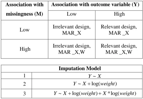
parametric MI in terms of robustness to different degrees of model misspecification. The comparison will be made under different scenarios, defined by the associations of the design variable (Z) used for determining the selection probabilities with both the outcome variable (Y) where missing data occur, and the latent variable (T) which defines the response mechanism.

The rest of this chapter is organized as follows. Section 2.2 provides a detailed overview of the proposed two-step semiparametric multiple imputation procedure. (We term it “semiparametric” because the design feature, in particular the weights, are

accommodated non-parametrically, whereas the actual imputation is conducted under a standard parametric model.) Section 2.3 discusses point estimation and inference using the MI datasets from the proposed procedure. Section 2.4 provides a simulation study in the context of a single-stage probability-proportional-to-size (PPS) sample design. We estimate population means and regression coefficients under settings where sampling weights are associated to differing degrees with both the outcome and the probability of

(34)

21

nonresponse, and where failure to account for design in the imputation procedure has differing degrees of impact. Section 2.5 applies the proposed procedure to estimate means, linear and loglinear regression models, and general location models describing marginal and joint distributions of income and health insurance accessibility. Section 2.6 discusses possible extensions to incorporate other design features beyond sampling weights, as well as extensions to deal with unit non-response weights.

2.2 A Two-Step Semiparametric MI Procedure 2.2.1 Overview and Notation

Bayesian finite population inference (Ericson 1969) has been proposed as a means to harmonize design- and model-based approaches for sample survey inference (Little 2004, 2011; Gelman 2007). Under this approach, we focus on the posterior predictive distribution of the finite population quantity of interest (e.g., population mean, population regression parameter) obtained from the posterior predictive distribution for the non-sampled elements of the population. To make matters more concrete, consider the setting where we have a scalar outcome Y, sampling weight w based on a single-stage PPS sampling design, and no missing data. Our complete data consist of the vector of sampling indicators I for the population, sampled Ysfor which I 1, the non-sampled Yns for which I 0, and similarly ws and wns. Given the sampling weights, the sampling mechanism generating I is assumed to be ignorable (p I Y w( | , )p I w( | )), and can be ignored in the modeling. Assuming a model for the outcome given the sampling weights

( | , )

p Y  w parameterized by  with prior p( ) , the posterior predictive distribution for the non-sampled elements of the population Yns is given by

(35)

22

( _ns| _s, _s) ( _ns| _s, , ) ( | _s, ) ( _ns| _s) _ns

p Y Y w 



p Y Y  w p Y w p w w d dw [2.1] Previous work has tackled estimation of this predictive distribution in a variety of manners. Zheng and Little (2003, 2005) and Chen, Elliott and Little (2010) assumed that the sampling weights were known for all subjects, so that ws w, reducing [2.1] to

( _ns| _s, ) ( _ns| _s, , ) ( | _s, )

p Y Y w 



p Y Y  w p  Y w d; these authors then obtained draws from the posterior predictive distribution under fairly weak modeling assumptions (parametric regression model for p Y( | , ) w based on penalized splines). Little and Zheng (2007) and

Zangeneh, Keener, and Little (2011) considered the situation in which weights (or

equivalently the size measure Z) are observed only for the sample (as in a public use data setting), and obtained predictive draws for p w( ns|ws) under a Dirichlet model with a

non-informative (Haldane) prior; the resulting predictive draw of the population of weights w was then used as covariates in Little and Zheng to obtain posterior predictive draws of Yns. Dong, Elliott, and Raghunathan (2014) consider a different factorization of [2.1]:

( _ns| _s, _s) ( _ns, _ns| _s, _s) ( ,_s _s) _ns

p Y Y w 



p Y w Y w p Y w dw [2.2] The parameter  is dropped because the draws of p Y w( ,_s _s) are made directly from the posterior of the empirical joint CDF of Y ws, susing a Bayesian bootstrap (BB) procedure (Rubin 1981). Draws from p Y( ns,wns|Y ws, s) are then made using a weighted finite

population Bayesian bootstrap (FPBB) procedure described in Cohen (1997).

Here we extend the approach of Dong, Elliott, and Raghunathan to accommodate missing data. We assume that, had we taken a census of the entire population, we could have observed a vector of response indicators R(R Rs, ns), where Rscorresponds to the response indicators observed in the sample, and R_nsto the response indicators associated

(36)

23

with the non-sampled elements. We then divide the sampled Y_s (Y_{s obs}_, ,Y_{s mis}_, ) into the fully-observed and missing elements, corresponding to the sampled Y values associated with Rs1 and Rs0 respectively, and similarly the non-sampled Yns(Yns obs, ,Yns mis, ) into those that would have been observed had they been sampled (Rns1), and those that

would have had missing values (Rns0). We also assume a fully-observable covariate ( s, ns)

X  X X consisting of the sampled and nonsampled elements respectively. Note that we can combine the observed from the sampled and nonsampled parts of the population to obtain the potentially “observable” Yobs (Ys obs, ,Yns obs, ), and similarly Ymis (Ys mis, ,Yns mis, ). We assume ignorable missingness, so that p R Y X w( | , , )p R Y( | obs,X w, ), allowing R to be

ignored in the model along with I. Extending [2.2] to incorporate item-level missingness (and thus the covariate X used for imputation) then yields

, , , ,

, , , , , ,

( , | , , ) ( , , | , , , ) ( , , , | , , , ) ( , , , )

ns ns s s s ns obs ns mis ns s obs s mis s s

ns obs ns mis ns ns s obs s mis s s s obs s mis s s ns

p Y X Y X w p Y Y X Y Y X w

p Y Y X w Y Y X w p Y Y X w dw

 



[2.3]

To obtain the posterior predictive distribution based on fully-observed data, we need to integrate the left side of [2.3] with respect to Y_mis (Y_{s mis}_, ,Y_{ns mis}_, ).

, , , , ,

( _{ns obs}, _ns| _{s obs}, _s, _s) ( _{ns obs}, _ns| _mis, _{s obs}, _s, _s) ( _mis| _{s obs}, _s, _s) _mis

p Y X Y X w 



p Y X Y Y X w p Y Y X w dY

To accomplish this, we reintroduce a parametric model for p Y( | , X w, ), and integrate out with respect to the posterior distribution of  :

, , ,

( _mis| _{s obs}, _s, _s) ( _mis| _{s obs}, _s, , _s) ( | _{s obs}, _s, _s)

p Y Y X w 



p Y Y X  w p Y X w d. Thus [2.3] becomes , , , , , , , , , , ( , | , , ) ( , | , , , ) ( | , , , ) ( | , , ) ( , | , , ) ( | , , , ) ( | , , ) ns obs ns s obs s s

ns obs ns mis s obs s s mis s obs s s s obs s s mis

ns obs ns s obs s s mis s obs s s s obs s s mis

p Y X Y X w p Y X Y Y X w p Y Y X w p Y X w d dY p Y X Y X w p Y Y X w p Y X w d dY        



[2.4]

(37)

24

observable) elements of the population are generated using the finite population Bayesian bootstrap.

A key result from [2.4] is that, since the unobserved elements of the population have been generated non-parametrically, we can implement the integration in [2.4] by use of a Gibbs sampler that iterates between obtaining draws of  conditional on the entire population, and draws of the missing data conditional on  and the observable elements of the population

( | , , , ) ( | , , ) ( | , , ) ( | , )

mis obs s mis obs s p Y Y X w p Y Y X p Y X w p Y X      

Since the nonparametric procedure generates draws from the joint posterior distribution of all variables for the nonsampled population, the relationships of the weights and other variables are maintained in the draws. It is thus sufficient to develop a parametric model for Y that does not involve the weights:p Y( | , X w, )p Y( | , X). This model does need to condition on weights, however, when the weights are further associated with the missing data mechanism.

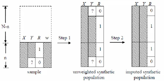
Figure 2.1 shows the creation of a single imputed synthetic population dataset under the proposed two-step MI procedure: a) shows the original sample data, b) the result from the BB-weighted FPBB procedure, and c) the result from the (model-based) imputation procedure. The shaded area represents observed data and ‘?’ represents

missing data. We discuss in detail the derivation and implementation of the proposed two-step MI procedure below.

(38)

25

a) b) c)

Figure 2.1 The procedure to create a single imputed synthetic dataset (Y: outcomes with item missing data; X: complete covariate; R: response indicator; w: sampling weight)

2.2.2 Step 1: Undo Sampling Weights through Synthetic Data Generation The Pólya’s Urn Scheme

The Polya urn distribution (Feller, 1968) is defined by construction as follows: suppose we have an urn containing a finite number n of balls of different colors. A ball is randomly drawn from the urn and another ball with the same color from outside of the urn is added back to the urn along with the originally picked one. Repeat this selection process until m balls have been selected; the resulting sample is termed a ‘Pólya sample of size m’.

The Pólya Posterior

The Polya posterior (Ghosh & Meeden, 1997) derives its name from the Polya urn distribution.It is a noninformative Bayesian procedure which can be used when little or no prior information is available.One advantage of the Polya posterior is that it has a stepwise Bayes justification (Hsuan, 1979) and leads to admissible procedures.

(39)

26

of size N. Let y_s { ,...,y₁ y_n} denote the sample, where y represents the realized value of a response variable Y. Let { ,d d₁ ₂,...,d_K} denote the set of K distinct values in the sample and { , ₁ ₂,...,_K} the vector of probabilities, such that Pr(y_i d_j| ) _j, for

1, 2,..., , 1,..., , i n j K and 1 1 K j j  



. Let n_j and ' j

n be the number of units taking value d_j in the sample and in the nonsampled part of the population, respectively, for

1, 2,..., ,

j K and



K_j_₁nj n,



K_j_₁n'j  N n. Assuming a noninformative Haldane

prior of : ~Dir(0,..., 0), 1 1 ( ) K j j p   





, together with a multinomial distribution for the counts of sample data: n₁,..,n_K |~Mult n( ; ) ,

1 1 1 1 ! ( ,..., | ) ! j j K K n n K K j j i j j j n p n n n       







, yields a Dirichlet posterior distribution of :

1 1 | ,...,n n_K ~Dir n( ,...,n_K)  , ₁ 1 1 ( | ,..., ) j K n K j j p  n n    



.

The Posterior predictive

distribution of counts in the nonsampled data thus follows a compound multinomial

distribution ' ' 1,..., K | 1,..., K ~ ( ; ) n n n n Mult Nn  : ' 1 1 1 _' _' 1 1 1 1 1 1 ' ' 0 0 1 1 1 1 1 1 1 1 1 0 0 1 1 1 ... ( ,..., | ,..., , ) ( ,..., | ) ( ) ... ( ,..., | ,..., ) ... ( ,..., | ) ( ) ... ... (1 ) j j K K K K K j K K _K K K j K n n j _j j p n n n n p n n p d d p n n n n p n n p d d                        



 



 



' 1 1 1 ₁ 1 1 1 0 0 1 1 1 1 1 1 1 1 1 1 0 0 ' 1 ... ... (1 ) ... ( ) / ( ) , ( ) / ( ) K K j K K _n _n K j K n K n j _j j K j K j j j j d d d d n n n N n        _ _                 



 





 



[2.5]

(40)

27

Ghosh and Meeden (1997) show that this posterior predictive distribution is in fact a Pólya urn distribution for the probability of seeing '

j

n balls with color d_j,

for j1, 2,...,K in some specified order. They also discuss the close relationship between the Polya posterior and the Dirichlet process priors (Ferguson, 1973) and the Bayesian bootstrap (BB) (Rubin, 1981). The Polya posterior is operationally and inferentially equivalent to the finite population Bayesian Bootstrap (FPBB) of Lo (1988),

which is just the BB adapted to finite population sampling problems.

The weighted Polya Posterior/weighted FPBB

Formula [2.5] can be generalized to the case when the sampled units bear different weights, i.e. when the realized sample is selected with unequal probabilities (Cohen, 1997). To be consistent with the specific PPS sample we are considering in this chapter, we adapt the notation as follows: denote the PPS sample as

( ,Y X w R_s _s, _s, _s) {( , Y X w R i_i _i, _i, _i), 1,..., .}n , where _i N _i _i i

w 



Z nZ for size variable Z and sample and population sizes n and N, and Y_i Y_{i obs}_, if R_i 1 and Y_i Y_{i mis}_, if Ri 0. Let

1 2

{ ,d d ,...,d_K} denote the set of K distinct vectors of ( ,Y X w R_i _i, _i, _i) in the sample and

1 2

{ , ,..., _K}

     the vector of probabilities that Pr ( ,



Y X w Ri i, i, i)dj|



j, for 1

1, 2,..., , 1,..., , and K _j 1

j

i n j K



_  . Let n_j and '

j

n be the number of units taking vector d_j in the sample and in the nonsampled part of the population, respectively, for

1, 2,..., , j K and ' 1 , 1 . K K j j j n n j n  N n



For convenience, assume that all

(41)

28

weight for the ith unit in the sample, which is normalized to sum up to N, i.e.

1 n i i w N  



.

Then w_i can be thought as the posterior expectation of the count of units in the population that have the same value as the ith unit in the sample. Again assuming a noninformative Haldane prior of  :  ~Dir(0,..., 0) together with multinomially distributed weighted counts in the data ₁

1 ( ,..., | ) j K w K j j p w w    



yields a Dirichlet posterior distribution of  : |w₁,...,w_K ~Dir w( ,...,₁ w_K),

1 1 1 ( | ,..., ) j K w K j j p  w w    



[2.6] The posterior predictive distribution of counts in the nonsampled data then follows a

compound multinomial distribution with an adjusted parameter

* * * 1 { ,..., _K}     , i.e. ' ' * 1,..., K | 1,..., K ~ ( ; ) n n w w Mult Nn  _: ' ' 1 1 1 * 1 1 * 1 * * 1 1 1 1 ' ' 0 0 1 1 1 1 1 * 1 1 * 1 * * 1 1 1 1 0 0 ' 1 ... ( ) (1 ) ... ( ,..., | ,..., ) ... ( ) (1 ) ... ( ) / ( ) j j K K j K K w n K w n j j j K j K K _K _w _K w j _j j K j K j j j j d d p n n w w d d w n w                                 





 





 



, (2Nn) / ( ) N [2.7]

In Little and Zheng (2007), *

( 1)

j C j wj

    

, for j1,..., .K , where C is a constant that satisfies

* 1

j j

 



; In this thesis, we follow the weighted Polya urn sampling suggested by Cohen (1997) and use a formula shown in equation [2.10].

The Adapted-weighted FPBB method

The adapted-weighted FPBB consists of two stages. The first stage resamples the original sample using the standard Bayesian bootstrap assuming IID, and the second

(42)

29

stage reverses/undoes the sampling weights using the weighted FPBB. This two-stage algorithm is similar in spirit to the standard parametric Bayesian method, where the first stage is equivalent to drawing values of the parameter ( ) from its posterior distribution given the counts in sampled data (n₁,...,n_K) and the second stage draws the predicted counts in the nonsampled data (n₁',...,n'_K) given the drawn parameter. Note that in Little and Zheng (2007), the first stage is replaced by drawing the parameter directly from a Dirichlet posterior distribution given by [2.6]. The method is described as follows:

 Resampling using the standard Bayesian Bootstrap (BB)

The standard Bayesian Bootstrap of Rubin (1981) assuming IID is used to

generate L replicate BB samples each of size n, i.e.



(Y_s( )l ,X_s( )l ,w( )_sl ,R_s( )l ),l1,..., .L



. This essentially generates the posterior of the empirical joint CDF (denoted by f ) of all the variables in the population given their realized values in the sample data set. Or

equivalently, the posterior distribution of the parameter vector  is drawn given the sample, i.e.













( ) ( ) 1 ( ) ( ) ( ) 1 , , , | ( , , , ) | , , , ~ ( ,..., ) for 1,..., ., where ,..., . l s s s s l s s s s K l l l K f Y X w R Y X w R Y X w R Dir n n l L        [2.8]

This stage captures the sampling variability. The uncertainty in the posterior

draws of the parameter ( )l is reflected in the varying counts of distinct units in the original sample being selected in different replicate BB samples. Let _l( )i denote the number of times unit i is selected in the lth replicate BB sample, for l1,..., .L We incorporate this source of uncertainty in computing “the lth bootstrap weight for unit i”,

(43)

30

i.e. w_i( )l w_i_l( )i , where w_i denotes the original sampling weight for unit i. Note that unequal inclusion probabilities still exist in these created BB samples. The bootstrap weights are carried forward as input weights to the next stage.

 Undo Sampling Weight using the weighted Polya posterior/weighted FPBB The weighted Polya poster

Accounting for Complex Sample Designs in Multiple Imputation Using the Finite Population Bayesian Bootstrap.