A simple and fast online power series multiplication and its analysis

A simple and fast online power series

multiplication and its analysis

∗

Romain Lebreton LIRMM UMR 5506 CNRS Université Montpellier II Montpellier, France Email:[email protected] Éric Schost

Computer Science Department Western University

London, Ontario Canada Email: [email protected]

Abstract

This paper focus ononline(orrelaxed) algorithms for the multiplication of power series over a field and their analysis. We propose a new online algorithm for the multiplication using middle and short products of polynomials as building blocks, and we give the first precise analysis of the arithmetic complexity of various online multiplications. Our algorithm is faster than Fischer and Stockmeyer’s by a constant factor; this is confirmed by our experimental results.

Keywords: Online algorithm, relaxed algorithm, multiplication of power series, arithmetic complexity

1 Introduction

Let A _{be a commutative ring with unity, and let x be an indeterminate over} A_. Given two power seriesa=P

i>0aix i_and b=P i>0bix i_{in A[[} x]], we are interested in computing the coefficients ci of the productc=a b under the following constraint: we

cannot use the coefficientsai orbi before we have computedc0,, ci−1. This condition

is useful to model situations where the inputs a, b and the output c are related by a feedback loop,i.e.where c0,, ci−1are needed in order to determineai andbi (see the

discussion below).

1 Previous work. Algorithms that satisfy such a constraint were introduced by Fischer and Stockmeyer in (Fischer and Stockmeyer, 1974); following that reference, we will call them online (the notion of an online algorithm extends beyond this question of power series multiplication, see for instance (Hennie,1966)). Still following Fischer and Stockmeyer, we will also consider half-line multiplication, where one of the arguments, sayb, is assumed to be known in advance at arbitrary precision; in other words, the only constraint for such algorithms is that we cannot use the coefficient ai before we have

computedc0,, ci−1.

∗. This work has been partly supported by the ANR grant HPAC (ANR-11-BS02-013), NSERC and

It seems that few applications of online power series multiplication were given at the time (Fischer and Stockmeyer, 1974) was written. Recently, van der Hoeven rediscov-ered Fischer and Stockmeyer’s half-line and online multiplications algorithms, which he respectively calledsemi-relaxed andrelaxed (Hoeven,1997;Hoeven,2002). In addition, as alluded to above, he showed that online multiplication is the key to computing power series solutions of large families of differential equations or of more general functional equations; this result was extended in (Berthomieu and Lebreton,2012) to further fam-ilies of linear and polynomial equations, showing the fundamental importance of online multiplication.

We complete this brief review of online multiplication by mentioning its adaptation to real numbers in (Schröder,1997) and its extension to the multiplication of p-adic integers in (Berthomieu et al.,2011).

The results of the papers (Fischer and Stockmeyer, 1974; Schröder, 1997; Hoeven, 1997;Hoeven,2002; Berthomieu et al., 2011) can be summarized by saying that online multiplication is slower than “classical” multiplication by at most a logarithmic factor. More precisely, let us denote byM_{(n)a function such that polynomials of degree at most} n−1inA_{[x]can be multiplied in}M_{(n)base ring operations. For instance, using the naive} algorithm givesM_{(n) =O(n}2₎, Karatsuba’s algorithm givesM_{(n) =O n}log2(3)_{and Fast}

Fourier Transform (FFT) techniques allow us to takeM_{(n)quasi-linear: in the presence} of roots of unity inA_{of orders 2}ℓ_{for any ℓ>0, FFT givesM(n) = 9·2}ℓ_ℓ+O(2ℓ_{) with}

ℓ=⌈log2(n)⌉(hence the behavior of a “staircase” function).

Then, the results in (Fischer and Stockmeyer,1974) and (Hoeven,1997;Hoeven,2002) show that half-line multiplication to precisionn,i.e.with input and output moduloxn_,

can be done in time H_{(n) =O} X k=0 ⌊log2(n)⌋ n 2kM(2 k₎ !

and that online multiplication to precisionn can be done in time O_{(n) =O(}H_{(n)). In} all cases, ifM_{(n)/nis increasing,}H_(n)isO(M_{(n)log(n)), since all terms in the sum are} bounded from above byM_{(n); for naive or Karatsuba’s multiplication,}H_{(n)is actually} O(M_{(n)). The algorithm introduced by van der Hoeven in (Hoeven, 2003) for half-line} multiplication improves on the one reported above by a constant factor.

2 Our contribution. In this paper, we introduce a simple and fast algorithm for online multiplication, based on the ideas from (Hoeven, 2003). We compare it to previous algorithms by giving the first precise analysis of the arithmetic complexity of the various online and half-line multiplication algorithms mentioned up to now. For this complexity measure, our algorithm is faster than Fischer and Stockmeyer’s by a constant factor; this is confirmed by our experimental results.

2.1 Polynomial multiplication algorithms. For the rest of this paper, we will con-sider the arithmetic cost of our algorithms, that is the number of basic additions and multiplications inA_{they perform. The algorithms in this paper rely on two variants of} polynomial multiplication, called middle and short products. In order to describe them, we introduce the following notation, used in all that follows: if a=P

iaix

i_{is inA[x]or}

A_{[[x]], andn, mare integers withm}>_{n, then we write}

anm=an+an+1x+

+am−1x m−n−1_,

so thatanmhas degree less than m−n.

Let a, b ∈ A_{[x] with b of degree less than n. Then, the middle product MP(a,} b, n) of a and b is defined as the part cn−12n−1 of the product c

8 a b, so that

deg (MP(a, b, n)) < n. Naively, the middle product is computed via the full mul-tiplicationc8(a bmodx

2n−1_)divxn−1_{, which is done in time2M(n) +O(n), but this} not optimal. Indeed, the middle product is closely related to thetransposed multiplica-tion(Bostan et al.,2003;Hanrot et al.,2004); precisely, it is a transposed multiplication, up to the reversal of polynomial b; we deduce using for instance a general theorem in (Bürgisser et al.,1997), or the algorithms in (Bostan et al.,2003;Hanrot et al.,2004), that the arithmetic costMP_{of the middle product MP(a, b, n)satisfies}

MP_{(n) =}M_{(n) +O(n).}

Let now a, b∈A_{[x] be both of degree less than n. The low short product, or just} short product, of a and b is denoted by SP(a, b, n)8 (a b)modx

n_{. Its variant, the}

high short product of a and b is denoted by HP(a, b, n)8 (a b) div x

n−1_{. The two} operations are closely related since HP(a, b, n) =rev2n−1(SP(revn(a),revn(b), n))where

revn(a)8x

n−1_{a(1/x)denotes the reversal of lengthnof the polynomialaof degree less} thann. Therefore, these two short products have the same arithmetic cost.

We denote bySP_{(n)the arithmetic cost of the short product at precision n, and by} CSP a constant such thatSP(n)6CSPM(n) +O(n)holds for alln∈N∗. Of course, we can always assumeCSP61, but the actual cost of the short product is hard to pin down: although the size of the output is halved, we seldomly gain a factor2 in the cost.

As always, it is easy to adapt the naive multiplication algorithm to compute only the first terms; in this case, we gain a factor two in the cost,i.e.we can takeCSP= 1/2. The paper (Mulders, 2000) published the first approach for having CSP < 1 for the cost function M_{(n) = n}log2(3), which is an approximation of the cost of Karatsuba’s multiplication, givingCSP=0.81; however, taking forM(n)theexact arithmetic cost of Karatsuba’s, the best known upper bound remainsCSP= 1 (Hanrot and Zimmermann, 2004). For an hybrid multiplication algorithm that uses the naive algorithm for small values and switches to Karatsuba’s method for larger values, the situation is better: for a threshold n0 =32, the bound SP∗_{(n) 60.57 M}∗_{(n) is proved for multiplicative}

complexity; it is beyond the scope of this paper to prove that this bound remains valid for arithmetic complexity (for the implementation of (Hanrot and Zimmermann, 2004), SP_(n)60.6M_{(n)is a realistic practical bound).}

No improvement is known for the short product based on FFT multiplication. However the FFT algorithm is designed to compute the result of the multiplication moduloxn₋₁

instead of moduloxn _{when nis a power of 2. More precisely, leta, b∈A[x] withb of}

degree less thannandc8a btheir product. Thenc0

n+cn2n−1=cmod(x

n_−1)can

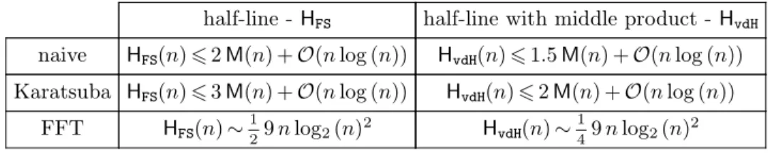
be computed within the number of arithmetic complexity of FFT multiplication in degree n/2whenn is a power of2. In any case, as will appear below, the overall contribution of short products will turn out to be negligible when we use FFT multiplication. 3 Our complexity results. Table1 gives bounds on the arithmetic complexity of half-linemultiplication algorithms depending on the algorithm we use to multiply truncated power series (naive, Karatsuba or FFT). In all the paper, we will often use the notation f(n)6g(n) +O(h(n))in our complexity statements for functions f , g, h:N_→N∗ _such

that there existsD∈R_>+_{0such that for alln∈}N_{, f(n)}6g(n) +D h(n).

The half-line multiplication algorithm which appears in (Fischer and Stockmeyer, 1974) gives the costs of the first column; we give an overview of this algorithm in Sec-tion2.1. The second column corresponds to the half-line algorithm using middle product presented in (Hoeven, 2003), which can be found in Section2.2. Table 1 sums up the results of Corollary14and Proposition18.

half-line - H_{FS half-line with middle product -}H_vdH naive H_FS(n)62M_{(n) +O(nlog(n))} H_vdH(n)6_1.5M_{(n) +O(nlog(n))} Karatsuba H_FS(n)63M_{(n) +O(n}log_(n)) H_vdH(n)62M_{(n) +O(n}log_(n))

FFT H_FS(n)∼1 29nlog2(n) 2 _H vdH(n)∼ 1 49nlog2(n) 2

Table 1. Complexity of half-line multiplication

Remark in particular that the cost of half-line algorithms using FFT polynomial mul-tiplication involves the function9nlog2(n), which is a smoothed version of the “staircase” cost function of the FFT mentioned above.

Table 2 describes online algorithms. The first column of Table 2 corresponds to the online multiplication algorithm of (Fischer and Stockmeyer, 1974; Hoeven, 1997; Berthomieu et al.,2011), which is presented in Section2.3. Our contribution, the online multiplication using middle and short products, gives the results of the second column and is presented in Section2.4. These complexity results are proved in Propositions15, 16and18.

online -O_{FS online with short and middle products -}O_LS naive O_FS(n)6M_{(n+ 1) +O(n}log_(n)) O_LS(n)6M_{(n+ 1) +O(n}log_(n)) Karatsuba O_FS(n)6_2.5M_{(n+ 1) +O(nlog(n))} O_LS(n)6 3 2CSP+ 1 _M (n+ 1) +O(nlog(n)) FFT O_{FS(n)∼9nlog2(n)}2 _O LS(n)∼ 1 29nlog2(n) 2

Table 2. Complexity of online multiplication

The factor beforeM_{(n+ 1)appearing for}O_{LSwith Karatsuba’s algorithm lies between} 1.75 for CSP=0.5 and 2.5 for CSP= 1. In practice, if we expect a behavior close to CSP=0.6 as in (Hanrot and Zimmermann,2004), we obtain a boundOLS(n)61.9M(n+

1) +O(nlog(n)).

In all cases, note that the bounds for our new algorithm O_{LS match, or compare} favorably to those forO_FS.

Remark 1. Recent progress has been made on online multiplication (Hoeven, 2007; Hoeven, 2012): these papers give an online algorithm that multiplies power series on a wide range of rings in time M_(n)log_(n)o(1), which improves on the costs given here. However, this algorithm is significantly more complex; we believe that there is still an interest in developing simpler and reasonably fast algorithms, such as the one given here.

Remark 2. It was remarked in (Hoeven, 1997; Hoeven, 2002) that Karatsuba’s multi-plication could be rewritten directly as an online algorithm, thus leading to a online algorithm with exactly the same numbers of operations. However, this algorithm is often not practical: the rewriting inducesΩ(log(n))function calls at each step, which makes it poorly suited to most practical implementations. For these reasons, we will not study this algorithm.

Remark 3. When the required precision nis known in advance, it is possible to adapt the online multiplication algorithms to this specific precision and thus lower the bounds given in Tables1and2 (seee.g.(Hoeven,2002;Hoeven,2003)).

Remark 4. We expect that our complexity results extend to online multiplication of p-adic integersZ_{p. In this case, one has to handle carries, but we believe that the resulting} extra cost should be only O(nlog(n)).

2 Description of the algorithms

In this section, we present our main algorithms for half-line and online multiplication; we postpone the detailed complexity analysis to the next section.

In all cases, we will use the following notational device. To compute a product of the forma b, either half-line or online, we will start from a “core” routine which takes as input aandb, as well as an extra inputc∈A_{[x]and a parameteri∈}N_{: the polynomialcstores} the current state of the multiplication and the integeri indicates at which step we are. Suppose thatAlgois such an algorithm, with input inA_[x]3_×Nand output inA_[x]; then, the main multiplication algorithmLoopAlgowill be the iterative process given as follows:

AlgorithmLoopAlgo

Input:a, b∈A_[x]andn∈N Output:c∈A_[x] 1. c= 0 2. forifrom 1ton a. c=Algo(a, b, c, i) 3. returnc

To state correctness, we will use the following properties(HL)and(OL), which express that LoopAlgois a half-line, respectively online, multiplication algorithm. The half-line

property reads as follows:

Property(HL).For anyn∈N_{and anya, b∈}A_{[x], the result c∈}A_{[x]of the} computa-tion LoopAlgo(a, b, n)satisfiesc=a b moduloxn. Moreover, during the computation, the

algorithm reads at most the coefficientsa0,, an−1of the input a.

Property(OL).Algorithm Algomust satisfy Property (HL)and, additionally, read at most the coefficients b0,, bn−1of the input b.

For all algorithms below, we first give a recursive version of the algorithm, which is easy to describe and applies when the target precisionnhas a special the form, such asn= 2k

orn= 2k_{−1. Then, we give the iterative form of the algorithms, obtained by “serializing”}

the recursion tree of the recursive algorithm (using iterative algorithms is necessary to fit in our framework ofLoopAlgoso that we can check properties (HL)or (OL)).

2.1 Fischer and Stockmeyer’s half-line algorithm

The first half-line multiplication algorithm was introduced in (Fischer and Stockmeyer,1974) by Fischer and Stockmeyer, and rediscovered by van der Hoeven in (Hoeven,1997;Hoeven,2002), up to a slight change in the recursion pattern.

We first give the recursive version of van der Hoeven’s variant. In its recursive form, the algorithm computesa b, with deg(a)< nand deg(b)< n−1, half-line ina,nbeing a power of two. Definea0=amodxn/2and a1=adivxn/2, as well asb0=bmodxn/2−1 andb1=bdivxn/2−1. Then, compute the following:

1. d08a0b0 (recursive half-line multiplication)

2. d08d0+a0b1x

n/2−1 _{(off-line multiplication)}

3. d08d0+a1b0x

n/2 _{(recursive half-line multiplication)} 4. d08d0+a1b1x

n−1 _{(off-line multiplication)}

One can verify the half-line constraints are maintained throughout this process. This recursive algorithm computes the full multiplicationa bat stepn= 2k_{. However, we will}

see that the property(HL)only guarantees that our product is correct modulonat other steps.

AlgorithmHalfline_FSbelow gives the iterative version of this algorithm; ais the online argument, andν2(n)denotes the 2-adic valuation of integer n.

Algorithm Halfline_FS Input: a, b, c∈A_[x]andi∈N Output: c∈A_[x] 1. forkfrom0 toν2(i) a. c=c+ai−2k ib2 k₋₁ 2 k+1₋₁xi−1 2. returnc

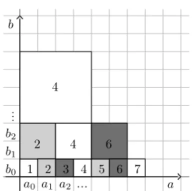
The diagram in Figure1shows the multiplications done when calling the iterative algo-rithm LoopHalfline_FS. The coefficients a0, a1, of a are placed in abscissa and the

coefficientsb0, b1, of bin ordinate. Each unit square corresponds to a product between

corresponding coefficients of a and b, i.e. the unit square whose left-bottom corner is at coordinates (i, j) stands for aibj. Each larger square corresponds to a product of

polynomials; ans×ssquare whose left-bottom corner is at coordinates(i, j)stands for aii+sbjj+s. The number inside the square indicates at which step iof LoopAlgothis

a b 1 2 3 4 5 6 7 2 4 6 4 a0 a1 a2 b0 b1 b2

Fig. 1. Fischer-Stockmeyer’s half-line multiplication

We can check on Figure 1 that for all n ∈ N_{, all the coefficients of the product}

P i=0

n−1P j=0

i

ajbi−jxi= (a·b)modxnare computed before or at stepn. We can also check

that the algorithm is half-line inasince at stepi, we use at most the coefficientsa0,,

ai−1of a, so AlgorithmHalfline_FSsatisfies Property(HL). However the operandbis off-line because, for example, the algorithm reads the coefficientsb0,, b6of bat step 4.

We will denote byH_{FS(n)the arithmetic complexity of algorithmLoopHalfline_FSwith} input precisionn,i.e.with input given moduloxn_.

Proposition 5. The following holds: H_{FS(n) =} X k=0 ⌊log2(n)⌋ jn 2k k M₍₂k_{) +O(nlog(n)).}

PROOF. We do at each step a product of polynomials of degree 0 which each costs M_{(1), hencensuch products to reach precisionn. Additionally, we do every other step,} starting from step 2, a product of polynomials of degree 1, which each costs M_{(2)for a} total of⌊n/2⌋M_{(2); generally, we do⌊n/2}k_{⌋products in degree2}k_{−1. Altogether, this}

accounts for the first term in the formula (note that the upper bound in the sum is the last value of k for which⌊n/2k_{⌋is nonzero).}

Keeping an exact count of all additions necessary to compute c is not necessary: at worst, each product with input size2k _incurs2k+1_{scalar additions to add its output to} c. If we write ℓ8⌊log2(n)⌋, the total is thus at most

X k=0 ⌊log2(n)⌋ j_n 2k k 2k+1₆X k=0 ℓ 2n, which isO(nlog(n)).

2.2 van der Hoeven’s half-line algorithm

Another half-line algorithm was introduced by van der Hoeven in (Hoeven, 2003). Whereas algorithm Halfline_FS used plain multiplication as a basic tool, this new

algorithm uses middle products. As before, this algorithm is half-line with respect to the inputa.

First, we give the recursive version; in this case, we have both deg (a) < n and deg(b)< n, for n of the form n= 2k _{−1. This time, we define a0=amodx}(n−1)/2_, a1=adivx(n+1)/2_andb0=bmodx(n−1)/2_{, so that all these polynomials have degree less} than2k−1_{−1; define as wella0}⋆_=amodx(n+1)/2_{. The algorithm does not compute the} producta b, but rathera bmodxn_{at stepsnof the formn= 2}k_{−1. It proceeds as follows:}

1. d08a0b0modx

(n−1)/2 _{(recursive half-line multiplication)} 2. d08d0+MP

a0⋆_{, b,}(n+ 1) 2

x(n−1)/2 _{(off-line middle product)} 3. d08d0+ a1b0modx

(n−1)/2

x(n+1)/2 _{(recursive half-line multiplication)} Again, one can check that the half-line constraints are maintained for the recursive calls.

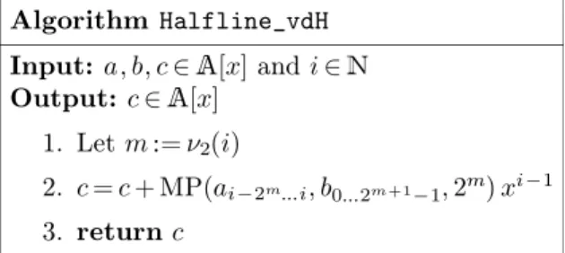
Since we compute only one middle product, whose size and cost are roughly those of one of the two multiplications done in the previous Subsection 2.1, we expect this algorithm to be faster than the previous one. To make this precise, we will analyze the iterative versionLoopHalfline_vdHof this algorithm, where subroutineHalfline_vdHlooks

as follows: Algorithm Halfline_vdH Input: a, b, c∈A_[x]andi∈N Output: c∈A_[x] 1. Letm8ν2(i) 2. c=c+MP(ai−2m i, b0 2 m+1₋₁,2m)xi−1 3. returnc

The mechanism of this algorithm is sketched in Figure2.

1 2 3 4 5 6 7 8 910 11 12 13 14 a b

One easily sees that AlgorithmHalfline_vdHsatisfies Property(HL), but the input argumentbis off-line because (for example) at step 2, the algorithm reads b0, b1, b2.

We will denote by H_{vdH(n) the arithmetic complexity of the half-line multiplication} algorithmLoopHalfLine_vdH, with target precisionn.

Proposition 6. The following holds: H_{vdH(n) =} X k=0 ⌊log2(n)⌋ n 2k+1+ 1 2 M₍₂k_{) +O(nlog(n)).}

PROOF. We claim that the cost of polynomial multiplications is given by

X k=0 ⌊log2(n)⌋ n+ 2k 2k+1 MP₍₂k_).

Indeed, as we can see on Figure2, for any integerk, we do a middle product of degree

2k_every2k+1_{th step, starting from step2}k_{. We saw before that in size2}k_{, the difference}

in cost between a middle product and a regular product is linear in2k_{; applying this to}

the above formula shows that the cost of polynomial multiplications is

X k=0 ⌊log2(n)⌋ n+ 2k 2k+1 M₍₂k_{) +O(} nlog(n)).

We must also take into account the additions of polynomials. Reasoning as in the proof of Proposition5, we see that the extra cost is O(nlog(n)).

2.3 Fischer and Stockmeyer’s online algorithm

We continue with the online multiplication algorithm due to Fischer and Stockmeyer, which is built upon their half-line algorithm. We first give the recursive version of this algorithm, foraandb of degree less thann, with nof the form2k_{−1. To computea b,}

online inaandb, definea0=amodx(n−1)/2anda1=adivx(n−1)/2, and define similarly b0andb1. Then, compute the following:

1. d08a0b0 (recursive online multiplication)

2. d08d0+a0b1x (n−1)/2 _{(half-line multiplication)} -. d08d0+a1b0x (n−1)/2 _{(half-line multiplication)} 3. d08d0+a1b1x n−1 _{(off-line multiplication)}

One can verify the online constraints are maintained throughout this process, provided the two half-line product are done “in parallel”. AlgorithmOnline_FS below gives the iterative version of this algorithm, that applies to anyn; as before, ν2(n)denotes the 2-adic valuation of integern.

Algorithm Online_FS Input: a, b, c∈A_[x]andi∈N Output: c∈A_[x] 1. forkfrom0 toν2(i+ 1) a. c=c+ai−2k ib2 k₋₁ 2 k+1₋₁xi−1 b. if(i+ 1 = 2k+1₎ returnc c. c=c+a2k₋₁ 2 k+1₋₁b_i−2k ix i−1 2. returnc

The following diagram sums up the computation made at each step by the iterative algorithmLoopOnline_FSand shows that it satisfies Property (OL).

1 2 3 4 5 6 2 3 _{3 5} 4 5 ₅ 7 8 9 10 7 9 7 6 7 8 9 7 9 10 a b

Fig. 3. Fischer and Stockmeyer’s online multiplication

We denote byO_{FS(n)the arithmetic cost induced by all operations done up to precision} n.

Proposition 7. The following holds: O_{FS(n) =} X k=0 ⌊log2(n+1)⌋−1 2 n+ 1 2k −3 M₍₂k_{) +O(nlog(n)).}

PROOF.For anyk>0, we do one product in degree2k_{−1at step2}k+1_{−1, then two such} products every2k_{th step. The total number of such products with target precisionnis}

n−(2k₋₁₎ 2k + n−(2k+1₋₁₎ 2k = 2 n+ 1 2k −3,

provided (n+ 1)/2k_{>2. This accounts for the first term in the above formula; as in}

the previous propositions, accounting for all polynomial additions induces the extra

2.4 A new online algorithm

The algorithm in the previous subsection relied on Fischer-Stockmeyer’s half-line algo-rithm to derive an online algoalgo-rithm. In this subsection, we show how using van der Hoeven’s half-line short product algorithm leads to a new online multiplication algorithm. As before, we start by giving the recursive version of the algorithm, which takes as inputaand b of degrees less thann, with this timenof the form 2k_{−2; the output is} (a b)modxn. We define nowa0=amodx(n−2)/2,a0⋆=amodxn/2anda1=adivxn/2, and similarly forb0,b0⋆andb1, and compute the following:

1. d08a0b0modx

(n−2)/2 _{(recursive online multiplication)} 2. d08d0+HP(a0

⋆

, b0⋆, n/2)x(n−2)/2 (off-line high product) 3. d08d0+ a0b1modx

n/2

xn/2 (half-line short product) -. d08d0+ a1b0modx

n/2

xn/2 (half-line short product) This gives us the following iterative algorithm, that is online with respect to inputs a andb. Algorithm Online_LS Input:a, b, c∈A_{[x] andi∈}N Output:c∈A_[x] 1. m=ν2(i+ 1) 2. if(i+ 1 = 2m₎ a. c=c+HP(a0i, b0i, i)x i−1 b. returnc 3. c=c+MP(ai−2m i, b0 2 m+1₋₁)xi−1 4. c=c+MP(bi−2m i, a0 2 m+1₋₁)xi−1 5. returnc 1 2 4 8 10 2 4 8 10 3 6 9 9 6 5 5 7 11 11 a b

Figure4sums up the computations of the iterative algorithmLoopOnline_LSand shows

that it satisfies Property (OL). Similarly to what we did in the previous sections, we denote byO_{LS(n)the cost of this algorithm with target precisionn.}

Proposition 8. The following holds: O_{LS(n) =} X k=1 ⌊log2(n+1)⌋ SP₍₂k _{− 1) + 2} X k=0 ⌊log2(n+1)⌋−1 n+ 1 2k+1 − 1 2 M₍₂k₎ ! + O(nlog(n)).

PROOF. The first term describe the short product in size2k_{−1that takes place at step} 2k _{−1. The second term comes from the fact that two middle products in size 2}k _are

done every2k+1_{steps, starting from step3·2}k_{−1, leading to a sum of terms of the form} n+ 2k+1_−(3·2k₋₁₎ 2k+1 = n+ 1 2k+1− 1 2 .

As usual, the extra additions add up to aO(nlog(n))term.

Remark 9. Even though there is no efficient short FFT multiplication algorithm, we can compute the short product of Step2efficiently. Indeed, we noticed in Section1that we can adapt the FFT multiplication to computec0n+cn2n−1wherec=a banda, bare

polynomials of length n. Since the partc0n was already computed by previous steps,

we can access tocn2n−1in half the time of a multiplication. However, we will see that

for FFT multiplication, the contribution of these short products is in any case negligible.

3 Complexity analysis

We introduce three auxiliary complexity functionsN_→N_{, defined as} M(1)_(n) 8 X k=0 ⌊log2(n)⌋ M₍₂k₎ M(2)_(n) 8 X k=0 ⌊log2(n)⌋ j n 2k k M₍₂k₎ M(3)_(n) 8 X k=0 ⌊log2(n)⌋ n 2k+1+ 1 2 M₍₂k₎ .

The cost of the previous algorithms can all be expressed using these functions.

Proposition 10. Up to a term inO(nlog(n)), H_{FS(n) =} M(2)_(n),

H_{vdH(n) =} M(3)_(n),

O_LS(n) 6 (CSP−2)M(1)(n+ 1) + 2M(3)(n+ 1).

PROOF.This is trivial forH_FSandH_vdHusing Propositions5and6. Propositions7and8 give us the formulas onO_{FS and}O_{LSby summing from0 toℓ=⌊log2(n+ 1)⌋instead of} from0 toℓ−1 and usingSP_(n)6CSPM(n) +O(n). In this section, we give bounds on these auxiliary functions. Since their behavior varies when M _{corresponds to a super-linear, resp. a quasi-linear function, we separate these} two cases and start with the case of superlinear functions.

Our objective is to give bounds that relate as closely as possible to practice. We choose not to assume thatM_{(n)/nis increasing, since this would not be satisfied for the} exact operation count of Karatsuba’s algorithm (this assumption would be satisfied if we used the upper boundM_{(n) =c n}log2(3)_{, for some suitable c, but since we want precise} estimates, we need to be more subtle).

3.1 Super-linear multiplication algorithms

In this subsection, we will make the following assumption.

Hypothesis (SL). The arithmetic cost function M _satisfies M_{(2n) =c}M_{(n) +a n+b} witha, b∈Z_{,c∈]2; +∞[ and} M_{(2n+ 1)−}M_(2n)>M₍₃₎₋M_{(2) forn}>1.

As we will see below, this framework includes both naive and Karatsuba’s algorithms, but it does not include Toom-Cook algorithms, nor the variant of Karatsuba’s algorithm that revert to the naive one for small values of n.

In the following lemmas, we use assumption(SL)to prove upper bounds on functions M(1)_(n),M(2)_(n)andM(3)_{(n). To this effect, define the constants}

a′ 8 a c−2, b ′ 8 b c−1 and e8|a ′_|+|b′_|,

as well as the functiond(λ)8M(λ) +a

′_λ+b′_{, forλinN.}

Lemma 11. Assumption (SL)implies that |M₍₂k_λ)−d(λ)ck_|6e2k_{λholds forλ∈N}∗_. PROOF.It suffices to unroll the recurrencektimes, and sum the geometric progressions:

M₍₂k_{λ) = cM(2}k−1_{λ) +a2}k−1_λ+b = ck_{M(λ) +a λ(2}k−1₊ +c k−1_{) +b(1 +} +c k−1₎ = ck_{M(λ) +}a λ(ck−2k) c−2 + b(ck₋₁₎ c−1 = ck M_{(λ) +} a λ c−2+ b c−1 −a2 k_λ c−2 − b c−1.

The conclusion follows immediately.

Remark in particular that the former lemma implies that|M₍₂k_)−d(1)ck_|=O(2k_).

Lemma 12. Let n be in N_{, with base-2 expansion given by n =} P i=0

ℓ

ni 2i, where

ℓ8⌊log2(n)⌋. Then, under assumption (SL), we have M(1)_{(n) =} c c−1M(2 ℓ_{) +O(n)} M(2)_{(n) =} c c−2 X i=0 ℓ niM(2i) +O(nlog(n)) M(3)_{(n) =} c−1 c−2 X i=0 ℓ niM(2i) +O(nlog(n)).

PROOF. In all that follows, we write for simplicity d 8 d(1) and M

(4)_{(n) =}

P i=0

ℓ

niM(2i). We start withM(1), applying the previous lemma to each summand: M (1)_(n)− c c−1M(2 ℓ₎ = X k=0 ℓ M₍₂k₎₋ c c−1M(2 ℓ₎ 6 X k=0 ℓ d ck₋ c c−1M(2 ℓ₎ +X k=0 ℓ e2k 6 c c−1d c ℓ₋ c c−1M(2 ℓ₎ + d c−1+e(2 ℓ+1₋₁₎ 6 c c−1e2 ℓ₊ d c−1+e(2 ℓ+1_−1), which amounts toO(n). Next, one has

M (2)_(n)− c c−2M (4)_(n) = X k=0 ℓ j_n 2k k M₍₂k₎₋ c c−2M (4)_(n) = X k=0 ℓ X i=k ℓ ni2i−kM(2k)− c c−2M (4)_(n) 6 X k=0 ℓ X i=k ℓ ni 2i−k d ck − c c−2 M (4)₍ n) + X k=0 ℓ X i=k ℓ ni2i−k(e2k) = X i=0 ℓ ni 2i d ( c/2)i+1₋₁ (c/2)−1 − c c−2 M (4)_(n) + O(nlog(n)) 6 (c/2) (c/2)−1 X i=0 ℓ nid ci− c c−2M (4)_(n) +O(nlog(n)) 6 O(nlog(n)). Finally, we have the inequalities

M(3)_(n)−c−1 c−2M (4)_(n) = X k=0 ℓ n 2(k+1) +nk M₍₂k₎₋c−1 c−2M (4)_(n)

6 X k=0 ℓ X i=k+1 ℓ ni 2i−(k+1) d ck − 1 c−2 M (4)_(n) + X k=0 ℓ X i=k+1 ℓ ni2i−(k+1)e2k = X i=1 ℓ ni 2i−1 d ( c/2)i₋₁ (c/2)−1 − 1 c−2 M (4)_(n) + O(nlog(n)) 6 (1/2) (c/2)−1 X i=0 ℓ nid ci− 1 c−2M (4)_(n) +O(nlog(n)) 6 O(nlog(n)).

The following inequality will allow us to control terms that appear in the estimates forM(2)_(n)andM(3)_{(n)given above. We introduce the notationC}8

d(3)−d(2)

d(1) .

Lemma 13. Let n be in N_{, with base-2 expansion given by n =} P i=0

ℓ

ni 2i, where

ℓ8⌊log2(n)⌋. Then, under assumption (SL), we have M₍₂ℓ_{) +C}X i=0 ℓ−1 niM(2i)6M(n) +O(nlog(n)). In particular, ifC>₁, we have X i=0 ℓ niM(2i)6M(n) +O(nlog(n)).

PROOF. The proof proceeds in three steps. First, we prove that the inequalityd(2n+ 1)−d(2n)>d(3)−d(2)holds for anyn>1. Indeed, we have thatd(2n+ 1)−d(2n) = M_{(2 n+ 1) −}M_{(2 n) +a}′_{, so the assumption M(2n + 1) −M(2n) >M(3)−M(2)}

establishes our claim. Next, we establish that for allk∈N_andm>1, we have M₍₂k+1_{m) +CM(2}k_)6M(2k+1_{m+ 2}k_{) +}

e′2k+1_m,

for somee′that does not depend onkorm. Indeed, Lemma11implies the inequalities M₍₂k+1_{m) +CM(2}k_{) 6 c}k_{(d(2m) +C d(1)) +e2}k_(2m+C)

ck_{d(2m+ 1) 6 M(2}k_{(2m+ 1)) +e2}k_{(2m+ 1).}

On the other hand, the inequality in the first paragraph implies thatd(2m) +C d(1)6

d(2m+ 1), and our claim follows by taking (for instance)e′=e(C+ 5)/2.

We can now prove the lemma. TakeninN_{, with base-2 coefficientsn0,}, nℓ. Applying

the above inequality withk=ℓ−1and m= 1yields M₍₂ℓ_{) +C n}

withn′= 2n. Adding the term C nℓ−2M(2ℓ−2)and applying the same inequality with k=ℓ−2 andm= 2 +nℓ−1, so that we still have2k+1m6n′, we get

M₍₂ℓ_{) +} X i=ℓ−2 ℓ−1 C niM(2i) 6 M(2ℓ+nℓ−12ℓ−1) +C nℓ−2M(2ℓ−2) +e′n′ 6 M₍₂ℓ_+n ℓ−12ℓ−1+nℓ−22ℓ−2) +e′(2n′). We can continue in this manner until we get M₍₂ℓ_{) +C}P

i=0

ℓ−1

niM(2i)6M(n) +e′ℓ n′,

which proves the lemma.

Corollary 14. Under assumption (SL) and ifC>1, one has H_FS(n)6 c

c−2M(n) +O(nlog(n)) and HvdH(n)6

c−1

c−2M(n) +O(nlog(n)) and these bound are asymptotically optimal since

H_FS(2m_)∼ c c−2M(2 m_{) and H} vdH(2m)∼ c−1 c−2M(2 m_).

PROOF.We deal withH_{FS(n)first. Using Proposition10, then Lemma12for the equality} below and Lemma13for the following inequality, we have that for alln∈N_,

H_{FS(n) =} c c−2 X i=0 ℓ niM(2i) +O(nlog(n)) 6 c c−2M(n) +O(nlog(n)).

Whenn= 2m_{, one has} H_FS(2m_{) =} c

c−2M(2

m_{) +O(nlog(n))∼} c

c−2M(2 m_).

The case ofH_{vdHis handled similarly.}

Proposition 15. Under assumption (SL)and if C>2c(c−1)

c+ 2 , one has O_FS(n)6 c+ 2

(c−2) (c−1)M(n+ 1) +O(nlog(n)) and this bound is asymptotically optimal, since

O_FS(2m_−1)∼ c+ 2

(c−2) (c−1)M(2 m_).

PROOF. Letℓ8⌊log2(n+ 1)⌋andn+ 1 = P

i=0

ℓ

ni2ibe the base-2 expansion of n+ 1.

Then, using Proposition10and Lemma12, one deduces O_{FS(n) = 2} c c−2 X i=0 ℓ niM(2i) +O(nlog(n)) ! −3 c c−1M(2 ℓ_{) +O(} n)+M₍₂ℓ₎ = 2c c−2− 3c c−1+ 1 M₍₂ℓ_{) +} 2·c c−2 X i=0 ℓ−1 niM(2i) +O(nlog(n))

= C1M₍₂ℓ_{) +C2}X i=0

ℓ−1

niM(2i) +O(nlog(n))

withC1=_(c−c_{2) (}+ 2_c−1) andC2=_c2₋·c₂. Provided that C2

C16

d(3)−d(2)

d(1) =C ,

we can then use Lemma 13 to deduce thatO_FS(n)6C1M_{(n+ 1) +O(nlog(n)). For} n+ 1 = 2m_{, all}

niare zero fori < ℓ, so one has O_FS(2m_{−1) =}

C1M₍₂m_{) +O(}

nlog(n))∼C1M₍₂m₎

.

Proposition 16. Under assumption (SL)and if C> 2 (c−1)2

c(c−2)CS P+ 2, one has

O_LS(n)6c(c−2)CSP+ 2

(c−2) (c−1) M(n+ 1) +O(nlog(n))

and these bounds are asymptotically optimal provided that SP₍₂k_−1)∼C

SPM(2k): O_LS(2m_−1)∼ m→∞c(c−2)C SP+ 2 (c−2) (c−1) M(2 m_).

PROOF. Letℓ8⌊log2(n+ 1)⌋andn+ 1 = P

i=0

ℓ

ni2ibe the base-2 expansion of n+ 1.

Using Proposition10and Lemma12, we deduce O_LS(n) 6 (CSP−2) c c−1M(2 ℓ_{)+ 2} c−1 c−2 X i=0 ℓ niM(2i) ! +O(nlog(n)) = C1′M(2ℓ) +C2′ X i=0 ℓ−1 niM(2i) +O(nlog(n)) withC1′=c(c−2)CS P+ 2 (c−2) (c−1) and C2 ′₌2 (c−1) c−2 . Provided that C2′ C1′ 6d(3)−d(2) d(1) =C ,

we can then use Lemma 13 to deduce thatO_LS(n)6C1′M_{(n+ 1) +O(n}log_(n)). For n+ 1 = 2m_{, alln}

iare zero fori < ℓ, so one has O_LS(2m_{−1) =}

C1′M₍₂m_{) +O(}

nlog(n))∼C1′M₍₂m₎

under the condition thatCSPis optimal in the senseSP(2k−1)∼CSPM(2k). Let us now verify that the naive and Karatsuba’s multiplication algorithms satisfy the

hypotheses of Corollary14and Propositions15and 16. Proposition15requires C>2c(c−1) c+ 2 = 4 ifc= 4 12/5 ifc= 3,

whereas Propositions16is verified whenever C> 2 (c−1) 2 c(c−2)/2 + 2= 3 if c= 4 16/7 if c= 3, sinceCSP>1/2.

4 Naive multiplication. The naive algorithm hasM_{(n) =n}2_{+ (n−1)}2_{= 2n}2_{−2n+ 1.} Using this expression, it is straightforward to verify that it satisfies hypothesis (SL), withM_{(2n) = 4}M_{(n) + 4n−3. Since}M_(n)∼2n2_andM(2k

λ)∼d(λ) 4k_{using Lemma11,} we getC=d(3)_d−₍₁₎d(2)=limk→∞ M(3·2k )−M(2·2k ) M(2k

) = 5. Therefore the naive multiplication satisfies the hypotheses of Corollary 14and Propositions 15 and 16. This gives us the first row of Tables1and2.

5 Karatsuba’s algorithm. Counting all operations, Karatsuba’s algorithm can be implemented usingK_{(n)operations, where}K_{(1) = 1and} K_{satisfies the following} recur-rence relation:

K_{(n) = 2}K_{(⌈n/2⌉) +}K_{(⌊n/2⌋) + 4n−4.}

The first two terms in the right-hand side require no justification, but we may say a few words about the linear term 4n−4. For instance, for n= 2m, writing a=a0+xm_a1

andb=b0+xm_{b1, we do2m additions prior to the recursive calls to computea0+a1}

and b0 + b1, 6 m − 3 additions and subtractions after the recursive call to compute

(a0+a1) (b0+b1)−a0b0−a1b1andm−1 additions to add that term to the result, for a total of8m−4 = 4n−4. The casen= 2m+ 1is similar.

In particular, we haveK_{(1) = 1,}K_{(2) = 7and}K_{(3) =23. For even inputs, this becomes} K_{(2n) = 3}K_{(n) + 8n−4, which show that the first part of our assumption is satisfied} and thata′= 8,b′=−2. Sinced(λ) =M_{(λ) +a}′_λ+b′_{, we getC=}d(3)−d(2)

d(1) =

45−13

7 =

32

7. Therefore Karatsuba’s multiplication satisfies the hypotheses of Corollary 14 and Propositions15and 16, from which we deduce the second row of Tables1 and2.

To prove the second item of(SL), we show by induction that for n>1, K_{(n+ 1)−} K_(n)>K₍₂₎₋K₍₁₎. Indeed, the case_{n= 1}is clear, and the inductive step follows from the equalities

K_{(n+ 1)−}K_{(n) =}

2 (K_{(n/2 + 1)−}K_{(n/2)) + 4 if neven} K_{((n−1)/2 + 1)−}K_{((n−1)/2) + 4 if nodd.} As claimed, we deduce that

K_{(2n+ 1)−}K_{(2n) = 2 (}K_{(n+ 1)−}K_{(n)) + 4}>2 (K₍₂₎₋K_{(1)) + 4 =}K₍₃₎₋K_(2). Remark that it is possible to save ⌊n/2⌋ − 1 redundant additions, see for instance Exercise 1.9 in (Brent and Zimmermann, 2011). This improved algorithm still satisfies

our assumptions, but our implementation does not use it. 3.2 Quasi-linear multiplication algorithms

Our previous analysis is not valid for quasi-optimal multiplication algorithms. In this section, we work under the following hypothesis.

Hypothesis(QL). There existsK∈R_{>0and (i, j)∈}N2_{such that} M₍₂k_)∼K2k_ki_log2(k)j_.

This hypothesis is verified by the fast Fourier transform algorithm which satisfiesM₍₂k_{) =} 9 · 2k _{k + O(2}k_{) under the condition that there exists enough 2}k_{th roots of unity}

(see (Gathen and Gerhard,2003)). Another suitable algorithm is the Truncated Fourier Transform because its cost coincides with the one of the FFT on powers of two (Hoeven, 2004). However, the Schönhage-Strassen multiplication algorithm does not fit in, as the ratioM₍₂k_)/(2k_{klog2(k))has no limit at infinity.}

Lemma 17. If M_{satisfies hypothesis (QL), then it verifies the following relations} M(1)_{(n) = O(}M_(n)), M(2)_{(n) ∼} 1 (i+ 1) n 2ℓM(2 ℓ_)log2( n), M(3)_{(n) ∼} 1 2 (i+ 1) n 2ℓM(2 ℓ_)log2(n).

PROOF. From hypothesis (QL), we getM(1)_(n)∼P k=0 ⌊log2(n)⌋ K2k_ki_(log2k)j_{. Because} P k=0 ℓ

K2k_ki_(log2k)j_{62 (K2}ℓ_ℓi_(log2ℓ)j_{) = 2M(n)whereℓ=⌊log2(n)⌋, we deduce our}

first point. Also, one has M(2)_{(n) =}X k=0 ℓ ⌊n/2k_⌋M(2k_{) =}X k=0 ℓ (n/2k_)M(2k_{) +O M}(1)_(n) . For the second point, notice thatM(2)_(n)−P

k=0

ℓ

(n/2k_)M(2k_{)is a big-O ofM}(1)₍ n)and so ofM_{(n)too. Conclude using the following equivalents forntends to infinity}

X k=0 ℓ (n/2k_)M(2k_{) ∼ K}X k=0 ℓ (n/2k_{) 2}k_ki_log 2 j (k) ∼ K n X k=0 ℓ ki_log 2 j (k) ! ∼ K n ℓi+1 i+ 1log2 j (ℓ) . Finally, we deal withM(3)_:

M(3)_{(n) =}X k=0 ℓ n 2k+1M(2 k_{) +O M}(1)_(n) ∼ 1 2 (i+ 1) n 2ℓM(2 ℓ_)log2(2ℓ_).

Proposition 18. Whenever M₍₂k_)∼K2k_klog2(k)j_{with j∈N, K∈R} >0, one has H_{FS(n) ∼} 1 2 n 2ℓM(2 ℓ_)log2(n), H_{vdH(n) ∼} 1 4 n 2ℓM(2 ℓ_)log2(n), O_{FS(n) ∼} n 2ℓM(2 ℓ_)log2(n), O_{LS(n) ∼} 1 2 n 2ℓM(2 ℓ_)log2(n), whereℓ=⌊log2(n)⌋.

PROOF.We use Lemma17and Proposition10forH_FS,H_vdHandO_{FS. For}O_{LS, we need to} go back to Proposition8to deduceO_{LS(n) = 2}M(3)_{(n+ 1) +O} M(1)_(n)

and our result.

TakingM₍₂ℓ_{) = 9·2}ℓ_ℓ+O(2ℓ_{), the previous proposition gives the third row of Tables1}

and 2 after a quick simplification. In particular, we remark that the cost n

2ℓ M(2

ℓ_{) is}

a smoothed version of M_{(n), especially for the “staircase” cost function of the FFT.} Indeed, the expression n

2ℓ M(2

ℓ_{) log2(2}ℓ_{) is equivalent to}

K nlog2(n)i_{log2 (log (}

n))j

under Hypothesis(QL). The equivalent simplifies further to an actualM_{(n)log2(n)for} the Truncated Fourier Transform algorithms or for quasi-linear evaluation interpolation schemes atnpoints.

4 Implementation and timings

We give timings of the different multiplication algorithms for the case of power series F_{p[[x]]with the 29-bit prime numberp=268435459. Computations were done on one core} of anIntel Core_{i7running at 3.6 GHz with 8Gb of RAM running a 64-bit}Linux_{. Our}

implementation uses the polynomial multiplication ofNTL _{6.0.0 (Shoup et al., 1990).}

The threshold between the naive and Karatsuba’s multiplications is at degree 16 and the one between Karatsuba’s and FFT multiplications at degree 600. Our middle product implementation is based on the implementation described in (Bostan et al.,2003).

In Figure5, we plot the timings in milliseconds of the multiplication of polynomials and of several online multiplication algorithms on power series depending on the precision in abscissa. The nameM_{stands for NTL’s multiplication, the name}H_{vdHstands for the} half-line multiplication using middle product of Section2.2, the nameO_{LSstands for the} online multiplication using middle (and short) product of Section2.4, and so on.

0 0.2 0.4 0.6 0.8 1 1.2 0 100 200 300 400 500 600 700 800 900 1000 Timings in milliseconds Precision O_FS H_FS O_LS H_vdH M

Fig. 5. Timings of different multiplication algorithms

Online algorithms are always slower than off-line algorithms since they have an addi-tional constraint. However, we will see that online algorithms are faster in very small precisions: this is because we compare online algorithms that compute short products a bmodxn_{at each step (and occasionally more, such as the full product forO}

FSandOLS whenn= 2ℓ_{) and an off-line algorithm that always compute the full producta b.}

We now draw the ratio of the timings of all online algorithms compared to NTL’s off-line multiplication. We give three figures depending on which off-line multiplication algorithm is used. We start with the naive algorithm used in precisions16n <16.

0.6 0.8 1 1.2 1.4 1.6 1.8 2 2.2 2.4 0 2 4 6 8 10 12 14 16 Ratio of timings Precision O_FS / M H_FS / M O_LS / M H_vdH / M

Fig. 6. Ratio of timings of different online products w.r.t. naive polynomial multipli-cation

For these small precisions, the ratio of timings do not follow our theoretical analysis. We reckon that cache effects or other low-level hardware specificities have a non-negligible effect on our timings. Still, we can notice from this figure that the variants using middle product always improve the online algorithms.

Let us turn to intermediate precisions corresponding to Karatsuba’s algorithm. NTL implements the variant of Karatsuba’s algorithm using the naive variant in small degrees for plain multiplication and we coded an odd/even decomposition for short product. Although Proposition 16 does not deal with this hybrid multiplication algorithm, we believe that the results for “pure” Karatsuba’s multiplication could apply in this case for nlarge enough and yield boundsO_FS62.5M_(n),H_FS63M_(n)andH_vdH62M_{(n), omitting} terms in O(n). Concerning our algorithm, the short product has a ratio CSP=0.6 in practice so we would expectO_LS6_1.9M_(n).

0.5 1 1.5 2 2.5 3 3.5 4 0 100 200 300 400 500 600 Ratio of timings Precision O_FS / M H_FS / M O_LS / M H_vdH / M

Fig. 7. Ratio of timings of different online products w.r.t. “hybrid” Karatsuba’s multi-plication

This plot confirms the theoretical bounds for Karatsuba’s multiplication, except on a few points forHvdH. Once again, the variants using middle product always improve online algorithms by a constant factor.

Finally for precision corresponding to FFT algorithm, the ratio grows with the preci-sion. Figure8shows the logarithmic growth of the ratio for precisionsn= 2ℓ_{. Note that}

NTL uses the 3-primes FFT algorithm on our field F_{p since it was lacking 2}ℓ_{th roots}

of unity (see (Gathen and Gerhard, 2003, Chapter 8.3)). This algorithm still matches Hypothesis(QL)in the range of degrees we consider and our analysis applies.

We can improve this analysis by plottingT_(n)/(n/2ℓ_M(2ℓ_{)log2(n)), whereTdenotes}

of the functionsH_{FS, ... that we are considering, expecting to observe constant ratios (in} theory, this ratio should tend to1for O_{FS, 1/2 for}H_FSandO_{LS, and 1/4 for}H_{vdH). This} is done in Figure9, where we observe a good agreement with theory.

In conclusion, we can see that the use of middle product always improves the perfor-mance of both the online and half-line multiplication algorithms. We save up to a factor

2 4 6 8 10 12 14 16 210 211 212 213 214 215 216 217 218 Ratio of timings Precision O_FS / M H_FS / M O_LS / M H_vdH / M

Fig. 8.Ratio of timings of online products w.r.t. FFT multiplication on precisionsN= 2ℓ

0.2 0.3 0.4 0.5 0.6 0.7 0.8 0.9 1 210 211 212 213 214 215 216 217 218

Constant in the equivalent

Precision O_FS

H_FS O_LS H_vdH

Fig. 9.Estimation of the constants in the equivalences of online product costs using FFT

Acknowledgements

We are grateful to P. Zimmermann for his thourough proofreading.

References

Berthomieu, J., Hoeven, J. v. d., Lecerf, G., 2011. Relaxed algorithms forp-adic numbers. J. Théor. Nombres Bordeaux 23 (3), 541–577.

Berthomieu, J., Lebreton, R., 2012. Relaxed p-adic Hensel lifting for algebraic systems. In: Proceedings of ISSAC’12. ACM Press, pp. 59–66.

Bostan, A., Lecerf, G., Schost, É., 2003. Tellegen’s principle into practice. In: Proceedings of ISSAC’03. ACM Press, pp. 37–44.

Brent, R., Zimmermann, P., 2011. Modern computer arithmetic. Vol. 18 of Cambridge Monographs on Applied and Computational Mathematics. Cambridge University Press, Cambridge.

Bürgisser, P., Clausen, M., Shokrollahi, M. A., 1997. Algebraic complexity theory. Vol. 315 of Grundlehren der Mathematischen Wissenschaften [Fundamental Principles of Mathematical Sciences]. Springer-Verlag, Berlin, with the collaboration of Thomas Lickteig.

Fischer, M. J., Stockmeyer, L. J., 1974. Fast on-line integer multiplication. J. Comput. System Sci. 9, 317–331.

Gathen, J. v. z., Gerhard, J., 2003. Modern Computer Algebra, 2nd Edition. Cambridge University Press, Cambridge.

Hanrot, G., Quercia, M., Zimmermann, P., 2004. The middle product algorithm. I. Appl. Algebra Engrg. Comm. Comput. 14 (6), 415–438.

Hanrot, G., Zimmermann, P., 2004. A long note on Mulders’ short product. J. Symbolic Comput. 37 (3), 391–401.

Hennie, F. C., 1966. On-line turing machine computations. Electronic Computers, IEEE Transactions on EC-15 (1), 35 –44.

Hoeven, J. v. d., 1997. Lazy multiplication of formal power series. In: ISSAC ’97. Maui, Hawaii, pp. 17–20.

Hoeven, J. v. d., 2002. Relax, but don’t be too lazy. J. Symb. Comput. 34 (6), 479–542. Hoeven, J. v. d., 2003. Relaxed multiplication using the middle product. In: Proceedings of the 2003 International Symposium on Symbolic and Algebraic Computation. ACM, New York, pp. 143–147 (electronic).

Hoeven, J. v. d., July 4–7 2004. The truncated Fourier transform and applications. In: Gutierrez, J. (Ed.), Proc. ISSAC 2004. Univ. of Cantabria, Santander, Spain, pp. 290– 296.

Hoeven, J. v. d., 2007. New algorithms for relaxed multiplication. J. Symbolic Comput. 42 (8), 792–802.

Hoeven, J. v. d., 2012. Faster relaxed multiplication. Tech. rep., HAL.

Mulders, T., 2000. On short multiplications and divisions. Appl. Algebra Engrg. Comm. Comput. 11 (1), 69–88.

Schröder, M., 1997. Fast online multiplication of real numbers. In: STACS 97 (Lübeck). Vol. 1200 of Lecture Notes in Comput. Sci. Springer, Berlin, pp. 81–92.

Shoup, V., et al., 1990. NTL: a library for doing number theory. Version 5.5.2. Available fromhttp://www.shoup.net/ntl/.