Modified maximum likelihood estimators using ranked set sampling

(1)

Contents lists available atSciVerse ScienceDirect

Journal of Computational and Applied

Mathematics

journal homepage:www.elsevier.com/locate/cam

Modified maximum likelihood estimators using ranked set sampling

Sibel Balci, Aysen D. Akkaya

∗

, B. Emre Ulgen

Statistics Department, Middle East Technical University, 06800, Ankara, Turkey

a r t i c l e i n f o

Article history: Received 14 April 2012

Received in revised form 22 August 2012 Keywords:

Order statistics

Modified maximum likelihood Ranked set sampling

a b s t r a c t

The closed-form maximum likelihood estimators (MLEs) of population mean and variance under ranked set sampling (RSS) do not exist since the likelihood equations involve nonlinear functions and have usually no explicit solutions. We derive modified maximum likelihood (MML) estimators for the population mean and variance under RSS and show that they are considerably more efficient than RSS estimators. Furthermore, we suggest two new estimators for the unknown parameters using two modified ranked set sampling methods and show that these methods make the variances of both MML and RSS estimators smaller.

In statistical parameter estimation problems, how well the parameters are estimated largely depends on the sampling algorithm used. Ranked set sampling is an innovative sampling design introduced in [1] in relation to estimating pasture yields. It has been widely used in agriculture, forestry, sociology, ecological and environmental sciences and medical studies. Ranked set sampling is a cost-efficient alternative to simple random sampling, particularly in situations where the measurements on the selected subject are difficult or expensive to obtain but ranking of the units according to the variable of interest is relatively easy and cheap [2].

LetX1

,

X2

, . . . ,

Xnbe a random sample of sizenwith probability density function (pdf)f

(

x

)

having mean

µ

and variance

σ

2_{. Ranked set sampling involves an initial ranking of}_n_{samples of size}_n_{as follows:}

Sample

1 X1(1) X1(2)

· · ·

X1(n−1) X1(n)

2 X2(1) X2(2)

· · ·

X2(n−1) X2(n)

...

n Xn(1) Xn(2)

· · ·

Xn(n−1) Xn(n).

Here,Xi(j)denotes thejth order statistic of theith random sample

(

i

=

1

,

2

, . . . ,

n

;

j

=

1

,

2

, . . . ,

n

)

. This phase is

followed by observing the first order statistic from the first sample,X1(1), the second order statistic from the second sample,

X2(2), and so on, until thenth order statistic from thenth sample,Xn(n), [3]. Thus,nobservations from then2sampling units

are measured and denoted byX1(1)

=

X[1]

,

X2(2)

=

X[2]

, . . . ,

Xn(n)

=

X[n].

McIntyre [1] proposed the following unbiased estimators for the population mean and variance:

ˆ

µ

RSS

=

n



i=1 X[i]

n with Var

(

µ

ˆ

RSS

) <

Var

(

¯

X

)

(1)

∗_{Corresponding author. Tel.: +90 312 2105329; fax: +90 312 2102959.}

E-mail address:[email protected](A.D. Akkaya).

(2)

and

ˆ

σ

2 RSS

=

n



i=1

(

X[i]

− ˆ

µ

RSS

)

2

/(

n

−

1

).

(2)

Also, Dell [4] and Dell and Clutter [5] showed that Var

(

µ

ˆ

_RSS

)

=

σ

2 n

−

n



i=1

(µ

[i]

−

µ)

2

/

n2

,

(3)

where

µ

[i]is the mean ofX[i].

Many studies about ranked set sampling have been made in the literature. McIntyre [1], in which ranked set sampling was developed, estimated pasture yields using this method. Halls and Dell [6] used it in sampling forage yields and showed that it was more efficient than random sampling. Also, Takahasi and Wakimoto [7] used this method assuming perfect ranking. Dell and Clutter [5] reviewed the ranked set sampling concept with particular consideration of errors in judgment ordering. Stokes [8] was interested in the estimation of variance. Stokes and Sager [9] studied the empirical distribution function based on ranked set samples and showed that it is an unbiased estimate of the underlying distribution function. Bohn and Wolfe [10,11] used the method to test for differences in the medians of two populations. Hettmansperger [12] computed a confidence limit on the median of a population, and Bhoj and Ahsanullah [13] obtained the estimates of the parameters of the generalized geometric distribution using a ranked set sampling procedure. Also ranked set sampling was used for estimating the slope and intercept of a straight line relation in [14], and estimating the means of several populations in an experimental setting in [15]. Density estimation using ranked set sampling data was considered in [16]. The procedures based on ranked set sample quantiles were tackled in [17]. Zheng and Al-Saleh [18] considered an alternative version of a maximum likelihood estimator (MLE) using RSS for general parameters, which has the same expression as the MLE using a simple random sample (SRS), except that the SRS in the MLE is replaced by the RSS.

We consider estimation of the population mean and variance under ranked set sampling by using the modified maximum likelihood method. The closed-form maximum likelihood estimators of these parameters under RSS do not exist since the likelihood equations involve nonlinear functions and are very difficult to solve even iteratively [19,20]. The modified maximum likelihood (MML) estimation method, originated in [21] and developed in [22], handles this problem. The MML estimators are (i) explicit functions of sample observations and are therefore easy to compute, (ii) considerably more efficient (unbiased and smaller variance) than the least squares estimators (LSEs) for all sample sizesn, particularly for largen, (iii) asymptotically fully efficient (unbiased and having minimum variances) under very general regularity conditions [23,24] and almost fully efficient for small samples, i.e., they have no or negligible bias and their variances are almost equal to the minimum variance bound, and (iv) robust to plausible deviations from the assumed distributions and to mild data anomalies (e.g. outliers) [25].

We derive MML estimators and compare them with competitors based on RSS. The efficiency properties of these estimators are investigated. Furthermore, we propose two new estimators for the population mean and variance using two modified ranked set sampling methods and show that these methods make the variances of both MML and RSS estimators smaller.

2. Modified maximum likelihood estimation

LetX[1]

,

X[2]

, . . . ,

X[n]be the ranked set sample from a location–scale distribution

(

1

/σ )

f

((

x

−

µ)/σ)

where

µ

and

σ

are location and scale parameters, respectively. Since the ranked set sample involves one order statistic from each of then

independent samples,X[i]

(

i

=

1

,

2

, . . . ,

n

)

are independent but not identically distributed. Moreover, marginallyX[i]and

X₍i)(ith order statistic in a sample of sizen) have the same distribution with pdf given by [26]

f

(

x[i]

)

=

n

!

(

i

−

1

)

!

(

n

−

i

)

!

σ



F



x[i]

−

µ

σ



i−1



1

−

F



x[i]

−

µ

σ



n−i f



x[i]

−

µ

σ



.

(4)

The likelihood function according to the ranked set sample is

L

∝

1

σ

n n



i=1



F

(

z[i]

)



i−1



1

−

F

(

z[i]

)



n−i f

(

z[i]

)

;

z[i]

=

x[i]

−

µ

σ

.

(5)

Here,F

(

x

)

is the cumulative distribution function of random variableX.

Suppose that the random variableXhas a normal distribution with mean

µ

and variance

σ

2_{. The likelihood equations}

for estimating

µ

and

σ

are given by

∂

lnL

∂µ

= −

1

σ

n



i=1

(

i

−

1

)

g1

(

z[i]

)

+

1

σ

n



i=1

(

n

−

i

)

g2

(

z[i]

)

−

1

σ

n



i=1 f′

(

_z [i]

)

f

(

z[i]

)

=

0 (6)

(3)

and

∂

lnL

∂σ

= −

1

σ

n



i=1

(

i

−

1

)

g1

(

z[i]

)

z[i]

+

1

σ

n



i=1

(

n

−

i

)

g2

(

z[i]

)

z[i]

−

1

σ

n



i=1 f′

(

_z [i]

)

f

(

z[i]

)

z[i]

−

n

σ

=

0

,

(7) where g1

(

z[i]

)

=

f

(

z[i]

)

F

(

z[i]

)

,

g2

(

z[i]

)

=

f

(

z[i]

)

1

−

F

(

z[i]

)

,

F

(

z[i]

)

=



z[i] −∞f

(

z[i]

)

dz[i]

,

f

(

z[i]

)

=

(

2

π)

−1/2exp

(

−

z[2i]

/

2

)

andf ′

(.)

is the derivative off

(.)

.

The likelihood equations(6)–(7)are expressions in terms of nonlinear functions,g1

(

z[i]

)

andg2

(

z[i]

)

, and have no explicit

solutions. Solving them by iteration is problematic [27,19]. The modified maximum likelihood estimation method overcomes these difficulties.

The method is implemented in three steps.

(i) The first step is to express the likelihood equations in terms of the ordered (in ascending order of magnitude) variates

z₍i)

=

((

y(i)

−

µ)/σ )

;

y(i)is theith order statistic obtained by ordering the ranked set sample,X[1]

,

X[2]

, . . . ,

X[n]. This is

accomplished by replacingz[i]byz(i)in(6)–(7).

(ii) The second step is to linearize the functionsg1

(

z(i))andg2

(

z(i))as

g1

(

z(i))

∼

=

α

1i

−

β

1iz(i) (8)

and

g2

(

z(i))

∼

=

α

2i

+

β

2iz(i). (9)

Here, the coefficients

α

1i

, α

2i

, β

1iand

β

2iare obtained by using the first two terms of the Taylor series expansions ofg1

(

z(i))

andg2

(

z(i))aroundt(i)

=

E

(

z(i)):

α

1i

=

f

(

t₍i)) F

(

t₍i))

+

t₍i)β1i

,

β

1i

=

t₍i)f

(

t(i))F

(

t(i))

+

f2

(

t(i)) F2

(

_t (i)) (10) and

α

2i

=

f

(

t₍i)) 1

−

F

(

t₍i))

−

t₍i)β2i

,

β

2i

=

f2

(

t₍i))

−

t(i)f

(

t(i))(1

−

F

(

t(i)))

(

1

−

F

(

t₍i)))2

.

(11) Although tables oft₍i)are available, it suffices to use their approximate values obtained from the equation



t(i)

−∞

f

(

z

)

dz

=

i

n

+

1

,

1

≤

i

≤

n

.

(12)

The modified likelihood equations denoted by

∂

lnL∗

/∂µ

=

_{0 and}

∂

_ln_L∗

/∂σ

=

_{0 are obtained by incorporating}₍₈₎_–₍₉₎_in

the likelihood equations:

∂

lnL∗

∂µ

= −

1

σ

n



i=1

(

i

−

1

)(α

1i

−

β

1iz(i))

+

1

σ

n



i=1

(

n

−

i

)(α

2i

+

β

2iz(i))

+

1

σ

n



i=1 z₍i)

=

0 (13) and

∂

lnL∗

∂σ

= −

1

σ

n



i=1

(

i

−

1

)(α

1i

−

β

1iz(i))z(i)

+

1

σ

n



i=1

(

n

−

i

)(α

2i

+

β

2iz(i))z(i)

+

1

σ

n



i=1 z₍2_i₎

−

n

σ

=

0

.

(14)

The solutions of the modified likelihood equations are the following MML estimators:

ˆ

µ

MML

=

1 m n



i=1

β

iy(i) and

σ

ˆ

MML

=

−

B

+

√

B2

+

₄_nC 2

√

n

(

n

−

1

)

,

(15) where

β

i

=

(

i

−

1

)β

1i

+

(

n

−

i

)β

2i

+

1

,

m

=

n



i=1

β

i

,

B

=

n



i=1

[

(

i

−

1

)α

1i

−

(

n

−

i

)α

2i

]

(

y(i)

−

K

),

(4)

Table 1 Means ofσˆMMLandσˆRSS. n E(σˆMML) E(σˆRSS) 5 0.9448 0.9224 6 0.9691 0.9398 7 0.9857 0.9534 8 0.9997 0.9675 9 1.0069 0.9722 10 1.0121 0.9752 Table 2

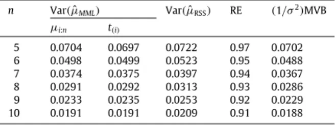
Exact variances ofµˆRSSandµˆMML, the REs ofµˆRSSand MVBs ofµˆMML:

σ=1. n Var(µˆMML) Var(µˆRSS) RE (1/σ2)MVB µi:n t(i) 5 0.0704 0.0697 0.0722 0.97 0.0702 6 0.0498 0.0499 0.0523 0.95 0.0488 7 0.0374 0.0375 0.0397 0.94 0.0367 8 0.0291 0.0292 0.0313 0.93 0.0286 9 0.0233 0.0235 0.0253 0.92 0.0229 10 0.0191 0.0191 0.0209 0.91 0.0188 C

=

n



i=1

[

(

i

−

1

)β

1i

+

(

n

−

i

)β

2i

+

1

]

(

y(i)

−

K

)

2

,

K

=

n



i=1

[

(

i

−

1

)β

1i

+

(

n

−

i

)β

2i

+

1

]

y(i) n



i=1

[

(

i

−

1

)β

1i

+

(

n

−

i

)β

2i

+

1

]

.

3. Properties of the MML and RSS estimators via simulation study

3.1. Unbiasedness

In this study, random samples have been generated from a standard normal distribution. MML and RSS estimators of the mean are unbiased estimators of

µ

because of the symmetry. The means of MML and RSS estimators of

σ

were simulated, and the simulations revealed that the bias in estimation of

σ

was negligible even for smalln. The results are given inTable 1;

σ

is taken to be equal to 1 without loss of generality.

It is seen fromTable 1that the means of MML and RSS estimators are very close to 1, which is the population variance, meaning that these estimators are unbiased.

3.2. Efficiency

The exact variances of

µ

ˆ

_RSSand

µ

ˆ

_MML, the relative efficiency (RE) values of

µ

ˆ

_RSS, RE

=

100

((

variance of

µ

ˆ

_MML

)/(

variance of

µ

ˆ

_RSS

))

and the Cramer–Rao minimum variance bound (MVB) values for

µ

ˆ

_MMLare given inTable 2. Note that Var

(

µ

ˆ

_MML

)

=

1

m2



n

i=1

β

i2

σ

i,i:n

,

Var

(

µ

ˆ

RSS

)

=

_n12



n

i=1

σ

i,i:n;

σ

i,j:n

=

Cov

(

z(i),z(j)), µi:n

=

E

(

z(i)) and

z₍i)

=

(

y(i)

−

µ)/σ

. The values of

µ

i:nand

σ

i,j:nare given in [28]. Here,

µ

i:nandt(i)are used alternatively for the calculation of

β

iin Var



ˆ

µ

MML



.

Table 2shows that Var



µ

ˆ

_MML



is smaller than Var



µ

ˆ

_RSS



and Var



µ

ˆ

_MML



is very close to the MVB, although sample sizes are small. Given inTable 3are the simulated variances of MML and RSS estimators of

σ

.

It is seen that the variance of

σ

ˆ

_MMLis smaller than that of

σ

ˆ

_RSS; the MML estimator of

σ

is more efficient. 4. MML and RSS estimators using two new sampling techniques

In this study, two new estimators for the population mean and variance using modified ranked set sampling methods (i) choosing both diagonal elements and (ii) choosing extremes of the samples have been developed in addition to MML estimators.

(5)

Table 3

Variances ofσˆMMLandσˆRSSestimators and REs ofσˆRSS.

n nVar ˆ σMML  nVar ˆ σRSS  RE 5 0.3423 0.3748 0.91 6 0.3227 0.3498 0.92 7 0.2993 0.3224 0.93 8 0.2875 0.3138 0.92 9 0.2673 0.2905 0.92 10 0.2497 0.2715 0.92

4.1. Ranked set sampling by choosing both diagonal elements

(

RSS

(

B

))

In this method,nsamples of sizenare taken, and each sample is ranked in itself as in ranked set sampling design: Sample

1 X1(1) X1(2)

· · ·

X1(n−1) X1(n)

2 X2(1) X2(2)

· · ·

X2(n−1) X2(n)

...

n Xn(1) Xn(2)

· · ·

Xn(n−1) Xn(n).

Here, both diagonal elements are chosen as a sample, i.e., the first and thenth order statistics are taken from the first sample:

X1(1)andX1(n); the second and the

(

n

−

1

)

th order statistics are taken from the second sample:X2(2)andX2(n−1); and so

on. Finally, thenth and the first order statistics are taken from thenthsample:Xn(1)andXn(n). The log-likelihood function

calculated for theith random sample is the joint pdf ofzi(i)

=

xi(i)−µ σ andzi(n−i+1)

=

xi(n−i+1)−µ σ : ln

(

Li

)

=

const

+

lnf

(

zi(i))

+

(

i

−

1

)

ln



F

(

zi(i))



+

(

n

−

2i

)

ln



F

(

zi(n−i+1))

−

F

(

zi(i))



+

lnf

(

zi(n−i+1))

+

(

i

−

1

)

ln



1

−

F

(

zi(n−i+1))



−

2 ln

σ .

(16)

The likelihood equation for estimating

µ

(location parameter) is

∂

lnLi

∂µ

= −

1

σ

f′

(

_z i(i)) f

(

zi(i))

−

(

i

−

1

)

σ

f

(

zi(i)) F

(

zi(i))

+

(

n

−

2i

)

σ

f

(

zi(i)) F

(

zi(n−i+1))

−

F

(

zi(i))







(1)

−

(

n

−

2i

)

σ

f

(

zi(n−i+1)) F

(

zi(n−i+1))

−

F

(

zi(i))

−

1

σ

f′

(

_z i(n−i+1)) f

(

zi(n−i+1))

+

(

i

−

1

)

σ

f

(

zi(n−i+1)) 1

−

F

(

zi(n−i+1))







(2)

=

0

.

(17)

Linearization of the parts(1)and(2)in Eq.(17)give (see Appendix 2A, [20,19])

∂

lnLi

∂µ

∼

=

∂

lnL∗_i

∂µ

=



α

i,i

+

β

i,izi(i)



+



α

_i_,_n−i+1

+

β

i,n−i+1zi(n−i+1)



=

0

.

(18)

Because of symmetry of(1)and(2),

α

i,n−i+1

= −

α

i,iand

β

i,n−i+1

=

β

i,i, in which caseE

(

∂ lnL∗

i

∂µ

)

=

0 as it should. Thus, the MML estimator of the population mean by choosing both diagonal elements of theith sample is

ˆ

µ

i

=

β

i,ixi(i)

+

β

i,ix(n−i+1) 2

β

i,i

=

xi(i)

+

xi(n−i+1) 2

.

(19)

For illustration, if we taken

=

5, we have the following. Sample 1:

µ

ˆ

₁

=

x1(1)+x1(5) 2 with Var

(

µ

ˆ

1

)

=

Var(x1(1))+Cov(x1(1)+x1(5)) 2

=

w

1

σ

2_. Sample 2:

µ

ˆ

₂

=

(

µ

ˆ

2

)

=

Var(x2(2))+Cov(x2(2)+x2(4)) 2

=

w

2

σ

2_.

Sample 3:

µ

ˆ

₃

=

x3(3)with Var

(

µ

ˆ

3

)

=

Var

(

x3(3))

=

w

3

σ

2.

Sample 4:

µ

ˆ

₄

=

(

µ

ˆ

4

)

=

Var(x4(4))+Cov(x4(4)+x4(2)) 2

=

w

4

σ

2

, w

4

=

w

2. Sample 5:

µ

ˆ

₅

=

(

µ

ˆ

5

)

=

Var(x5(5))+Cov(x5(5)+x5(1)) 2

=

w

5

σ

2

, w

5

=

w

1.

Each

µ

ˆ

_iis independent and unbiased. The MML estimator (unbiased and MVB) of the population mean obtained by using the RSS

(

B

)

method is

ˆ

µ(

B)

=

5



i=1



µ

ˆ

i

w

i

 

5



i=1



1

w

i



(20)

(6)

with E

(

µ(

ˆ

_B))

=

µ

and Var

(

µ(

ˆ

_B))

=

σ

2



5



i=1

(

1

/w

i

),

where

w

i

=

σi,i:n +_σi,n−i+1:n 2 and

σ

i,n−i+1:n

=

Cov

(

zi(i),zi(n−i+1)).

The RSS estimator of the population mean by using the RSS

(

B

)

method is given as follows:

ˆ

µ

RSS(B)

=











1

(

2n

−

1

)

[

(

x1(1)

+

x1(5))

+

(

x2(2)

+

x2(n−1))

+ · · ·

+

x₍n+1)/2((n+1)/2)

+ · · · +

(

xn(n)

+

xn(1))

]

ifnis odd

.

1 2n

[

(

x1(1)

+

x1(5))

+

(

x2(2)

+

x2(n−1))

+ · · ·

+

(

xn−1(n−1)

+

xn−1(2))

+

(

xn(n)

+

xn(1))

]

ifnis even

.

(21)

The estimators

σ

ˆ

_iare

ˆ

σ

1

=

x1(5)

−

x1(1)

2

µ

5:n

and Var

(

σ

ˆ

₁

)

=

Var

(

x1(1))

−

Cov

(

x1(1),x1(5)) 2

µ

2₅:n

=

v

₁

σ

2

, µ

2₅_:_n

=

µ

2₁_:_n

.

ˆ

σ

2

,

σ

ˆ

4and

σ

ˆ

5can be found similarly, and

σ

ˆ

3is equal to zero.

The unbiased and MVB estimator of

σ

and its variance obtained by using the RSS

(

B

)

method are

ˆ

σ(

B)

=

5



i=1



σ

ˆ

i

v

i

 

5



i=1



1

v

i



and Var

(

σ

ˆ

_B

)

=

σ

2



5



i=1

(

1

/v

i

),

(22) where

v

i

=

σi,i:n −σi,n−i+1:n µ2 n−i+1:n and

µ

i:n

=

E

(

zi(i)).

Note that the MML estimator of

σ

can be found by using a different procedure and thus it is not given here.

4.2. Ranked set sampling by choosing extremes of the samples

(

RSS

(

E

))

Here,nsamples of sizenare taken and each sample is ranked in itself as in ranked set sampling design. Then the smallest and largest order statistics from each sample are observed. This procedure can be described in a table as follows:

Sample

1 X1(1) X1(2)

· · ·

X1(n−1) X1(n)

2 X2(1) X2(2)

· · ·

X2(n−1) X2(n)

...

n X_n₍₁₎ Xn(2)

· · ·

Xn(n−1) Xn(n).

SinceXi(1)andXi(n)

(

i

=

1

,

2

, . . . ,

n

)

are used as the random sample, the likelihood function is the product of the joint pdf

ofXi(1)andXi(n): L

∝



1

σ



2n n



i=1 f

(

zi(1))



F

(

zi(n))

−

F

(

zi(1))



n−2 f

(

zi(n)), (23) where zi(j)

=

xi(j)

−

µ

σ

(

i

=

1

,

2

, . . . ,

n

;

j

=

1

,

n

).

The likelihood equations for estimating

µ

and

σ

(location and scale parameters) are

∂

lnL

∂µ

=

1

σ

n



i=1



zi(1)

+

zi(n)



+

(

n

−

2

)

σ

n



i=1



g

(

zi(1))

−

g

(

zi(n))



=

0 (24) and

∂

lnL

∂σ

= −

2n

σ

+

1

σ

n



i=1



z_i2₍₁₎

+

z2_i₍_n₎



+

(

n

−

2

)

σ

n



i=1



z_i₍₁₎g

(

z_i₍₁))

−

z_i₍_n₎g

(

z_i₍_n))



=

0

,

(25) where g

(

zi(j))

=

f

(

zi(j))

(

F

(

zi(n))

−

F

(

zi(1)))

(

i

=

1

,

2

, . . . ,

n

;

j

=

1

,

n

).

(7)

Akkaya and Tiku [29] showed thatF

(

zi(n))

−

F

(

zi(1))tends to its expected value quickly; that is, P

=

F

(

t2

)

−

F

(

t1

)

=

n

−

1 n

+

1

;

F

(

t1

)

=

1 n

+

1 and F

(

t2

)

=

1

−

1 n

+

1

=

n n

+

1

;

t₁

(

t₂

= −

t₁

)

is the solution of



t1 −∞ 1

√

2

π

e −z2/2_dz

=

1 n

+

1

.

The linearizedg

(

zi(1))andg

(

zi(n))are

g

(

z_i₍₁))

∼

=

α

₁

+

β

₁z_i₍₁₎ and g

(

z_i₍_n))

∼

=

α

₂

−

β

₂z_i₍_n). (26) Here,

α

1

=

α

2

=

α

and

β

1

=

β

2

=

β,

where

α

=

f

(

0

)

P and

β

=

f

(

t

)

−

f

(

0

)

tP

, (

t

=

t1

)

;

f

(

0

)

=

1 2

π

;

f

(

t

)

=

1

√

2

π

e −t2_/₂

.

The solutions of the modified likelihood equations are the following MML estimators obtained by using the RSS

(

E

)

method:

ˆ

µ(

E)

=

1 n n



i=1

ˆ

µ

i

,

µ

ˆ

i

=

xi(1)

+

xi(n) 2

(

i

=

1

,

2

, . . . ,

n

)

(27) and

ˆ

σ(

E)

=

−

B

+

√

B2

+

₈_nC 4n

.

(28)

Note that

µ(

ˆ

_E₎

= ˆ

µ

_RSS₍_E₎

=

µ

∗_and

Var

(

µ(

ˆ

_E))

=

1 n2 n



i=1 1 2



Var

(

xi(1))

+

Cov

(

xi(1),xi(n))



σ

2

,

₍₂₉₎

where

µ

ˆ

_RSS₍_E₎is the RSS estimator of

µ

and

µ

∗_{is the best linear unbiased estimator (BLUE) of}

µ

_{. However,}

σ(

ˆ

E)is different

from the BLUE of

σ(σ

∗

)

_.

The BLUE of the vector

θ

of parameters restricts estimates to be linear:

θ

∗

=

WX. SinceE

(

Xi(j))

=

µ

+

σ µ

j:n

(

i

=

1

,

2

, . . . ,

n

;

j

=

1

,

n

)

under the RSS

(

E

)

method, it can be formulated as a linear model:

X

=

W

θ

+

e

,

(30) where X

=







X1(1) X1(n) X2(1) X2(n)

...

Xn(1) Xn(n)







(2n)×1

,

W

=







1

−

µ

_n:n 1

µ

n:n 1

−

µ

_n:n 1

µ

n:n

...

1

−

µ

_n:n 1

µ

n:n







(2n)×2

,

θ

∗

=



µ

∗

σ

∗



and e

=







e1 e2

...

e2n







.

Here, the errorseiare not independently distributed. In fact, their variance–covariance matrix is

V

=







σ

n,n:n

−

σ

1,n:n 0 0

· · ·

0 0

−

σ

₁_,_n:n

σ

n,n:n 0 0

· · ·

0 0 0 0

σ

n,n:n

−

σ

1,n:n

· · ·

0 0 0 0

−

σ

₁_,_n:n

σ

n,n:n

· · ·

0 0

...

0 0 0 0

· · ·

σ

_n_,_n:n

−

σ

1,n:n 0 0 0 0

· · ·

−

σ

₁_,_n:n

σ

n,n:n







(2n)×(2n)

.

(31)

To obtain the BLUE of

µ

and

σ

, we minimize the generalized error variance [30]

(8)

Table 4

Variances ofµˆRSS,µˆMML,µˆRSS(B),µˆ₍B),µˆRSS(E),µˆ₍E)andµ∗

.

n Var(µˆRSS) Var(µˆMML) Var(µˆRSS(B)) Var(µˆ(B)) Var(µˆRSS(E))=Var(µˆ(E))=Var(µ∗)

5 0.0722 0.0704 0.0521 0.0505 0.0522 6 0.0523 0.0498 0.0358 0.0355 0.0394 7 0.0397 0.0374 0.0278 0.0269 0.0312 8 0.0313 0.0291 0.0211 0.0207 0.0256 9 0.0253 0.0233 0.0174 0.0167 0.0216 10 0.0209 0.0191 0.0139 0.0136 0.0186 Table 5

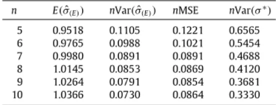
Means, variances and MSEs ofσˆ₍E)and the variances ofσ∗

. n E(σˆ₍E)) nVar(σˆ₍E)) nMSE nVar(σ∗₎

5 0.9518 0.1105 0.1221 0.6565 6 0.9765 0.0988 0.1021 0.5454 7 0.9980 0.0891 0.0891 0.4688 8 1.0145 0.0853 0.0869 0.4120 9 1.0264 0.0791 0.0854 0.3681 10 1.0366 0.0730 0.0864 0.3330

This gives the BLUE

θ

∗:

θ

∗

=



µ

∗

σ

∗



=

(

W′V−1W

)

−1W′V−1X

.

(33)

The right-hand side yields two linear functions,

µ

∗

=

1 2n n



i=1

(

Xi(1)

+

Xi(n)) and

σ

∗

=

1 n n



i=1

σ

∗ i

;

σ

∗ i

=

xi(n)

−

xi(1) 2

µ

n:n

with Var

(σ

_i∗

)

=

Var

(

xi(n))

−

Cov

(

xi(n),xi(1)) 2

µ

n:n

σ

2

.

₍₃₄₎

5. Comparison of RSS and MML methods

Table 4gives the exact variances of the RSS and MML estimators of population mean obtained by the RSS, RSS

(

B

)

and RSS

(

E

)

methods. The variances of BLUE obtained by using the RSS

(

E

)

method for the population mean are also given in the same table.Table 4indicates the following. (i) The MML estimator of

µ

is more efficient than the RSS one. Furthermore, the RSS estimator is inadmissible with squared error loss since both the RSS and the MML estimators are unbiased but the RSS estimator has bigger variance. (ii) The MML estimators are more efficient than the RSS estimators under the RSS

(

B

)

and RSS

(

E

)

methods. (iii) The MML and RSS estimators obtained by using the RSS

(

B

)

method are more efficient than the MML and RSS estimators obtained by using the RSS

(

E

)

method. (iv) The MML estimator obtained by using the RSS

(

B

)

method is the most efficient estimator.

In addition,Table 5gives simulation results for the mean, variance and mean square error (MSE) of the MML estimator for the population variance obtained by using the RSS

(

E

)

method. The variances of the BLUE of the population variance are also given inTable 5.

Table 5shows that the MSE for the MML estimator of population variance obtained by using the RSS

(

E

)

method is very small and that the variance of this estimator is also smaller than the variance of the BLUE.

Conclusion

Using the method of modified maximum likelihood under ranked set sampling, we obtained more efficient estimators for the population mean and variance for a normal distribution. We proposed two new estimators for the mean and variance of population using two modified ranked set sampling methods and showed that these methods make the variances of both MML and RSS estimators smaller and provide more efficient estimators. Estimators for the population mean and variance are also obtained for a long-tailed symmetric (LTS) distribution. The results are similar to those of a normal distribution, but are not given here for conciseness.

(9)

Acknowledgment

Some parts of this research work represented in this manuscript are supported by project no: BAP-08-11-DPT2002K120510, METU, Ankara, 2005.

References

[1] G.A. McIntyre, A method for unbiased selective sampling, using ranked sets, Aust. J. Agric. Res. 3 (1952) 385–390.

[2] P. Yu, Nonparametric estimation in ranked set sampling with concomitant variables, in: Combinatorics and Related Areas and the Eighth International Conference of Forum for Interdisciplinary Mathematics, 2001.

[3] N.A. Mode, L.L. Conquest, D.A. Marker, Ranked set sampling for ecological research: accounting for the total costs of sampling, Environmetrics 10 (1999) 179–194.

[4] T.R. Dell, The theory of some applications of ranked set sampling, Ph.D. Thesis, University of Georgia, Athens, GA, 1969. [5] T.R. Dell, J.L. Clutter, Ranked set sampling theory with order statistics background, Biometrics 28 (1972) 545–553. [6] L.S. Halls, T.R. Dell, Trial of ranked set sampling for forage yields, For. Sci. 12 (1) (1966) 22–26.

[7] K. Takahasi, K. Wakimoto, On unbiased estimates of the population mean based on the sample stratified by means of ordering, Ann. Inst. Statist. Math. 20 (1968) 1–31.

[8] S.L. Stokes, Estimation of variance using judgement ordered ranked-set samples, Biometrics 36 (1980) 35–42.

[9] S.L. Stokes, T. Sager, Characterization of a ranked set sample with application to estimating distribution functions, J. Amer. Statist. Assoc. 83 (402) (1988) 374–381.

[10] L.L. Bohn, D.A. Wolfe, Nonparametric two-sample procedures for ranked-set samples data, J. Amer. Statist. Assoc. 87 (1992) 552–561.

[11] L.L. Bohn, D.A. Wolfe, The effect of imperfect judgment rankings on properties of procedures based on the ranked-set samples analog of the Mann–Whitney–Wilcoxon statistic, J. Amer. Statist. Assoc. 89 (1994) 168–176.

[12] T.P. Hettmansperger, The ranked-set sampling sign test, J. Nonparametr. Stat. 4 (1995) 263–270.

[13] D.S. Bhoj, M. Ahsanullah, Estimation of parameters of the generalized geometric distribution using ranked set sampling, Biometrics 52 (1996) 685–694. [14] H.A. Muttlak, Parameters estimation in a simple linear regression using rank set sampling, Biom. J. 37 (1995) 799–810.

[15] H.A. Muttlak, Estimation of parameters for one-way layout with rank set sampling, Biom. J. 38 (1996) 507–515. [16] Z. Chen, Density estimation using ranked-set sampling data, Environ. Ecol. Stat. 6 (1999) 135–146.

[17] Z. Chen, On ranked-set sample quantiles and their applications, J. Statist. Plann. Inference 83 (2000) 125–135.

[18] G. Zheng, M.F. Al-Saleh, Modified maximum likelihood estimators based on ranked set samples, Ann. Inst. Statist. Math. 54 (3) (2002) 641–658. [19] D.C. Vaughan, The generalized secant hyperbolic distribution and its properties, Commun. Stat.—Theory Methods 31 (2002) 219–238. [20] M.L. Tiku, A.D. Akkaya, Robust Estimation and Hypothesis Testing, New Age International Publishers (P), New Delhi, 2004.

[21] M.L. Tiku, Estimating the mean and standard deviation from a censored normal sample, Biometrika 54 (1967) 155–165.

[22] M.L. Tiku, R.P. Suresh, A new method of estimation for location and scale parameters, J. Statist. Plann. Inference 30 (1992) 281–292.

[23] G.K. Bhattacharyya, The asymptotics of maximum likelihood and related estimators based on type II censored data, J. Amer. Statist. Assoc. 80 (1985) 398–404.

[24] D.C. Vaughan, M.L. Tiku, Estimation and hypothesis testing for a non-normal bivariate distribution with applications, Math. Comput. Modell. 32 (2000) 53–67.

[25] M.L. Tiku, W.Y. Tan, N. Balakrishnan, Robust Inference, Marcel Dekker, New York, 1986. [26] H.A. David, Order Statistics, second ed., John Wiley, New York, 1981.

[27] S. Puthenpura, N.K. Sinha, Modified maximum likelihood method for the robust estimation of system parameters from very noisy data, Automatica 22 (1986) 231–235.

[28] E.S. Pearson, H.O. Hartley, Biometrika Tables for Statisticians, Vol. II, Cambridge University Press, Cambridge, 1972.

[29] A.D. Akkaya, M.L. Tiku, Robust estimation and hypothesis testing under short-tailedness and inliers, TEST 14 (1) (2005) 129–150. [30] E.H. Lloyd, Least squares estimators of location and scale parameters using order statistics, Biometrika 39 (1952) 88–95.

Journal of Computational and Applied Mathematics 238 (2013) 171–179

SciVerse ScienceDirect