The operational matrices of Bernstein polynomials for solving the parabolic equation subject to specification of the mass

(1)

Contents lists available at

ScienceDirect

Journal of Computational and Applied

Mathematics

journal homepage:

www.elsevier.com/locate/cam

The operational matrices of Bernstein polynomials for solving the

parabolic equation subject to specification of the mass

S.A. Yousefi

a

, M. Behroozifar

b

, Mehdi Dehghan

c

,

∗

a_{Department of Mathematics, Shahid Beheshti University, G.C., Tehran, Iran} b_{Faculty of Basic Sciences, Babol University of Technology, Babol, Mazandaran, Iran}

c_{Department of Applied Mathematics, Faculty of Mathematics and Computer Sciences, Amirkabir University of Technology, No. 424 Hafez Avenue, Tehran, Iran}

a r t i c l e

i n f o

Article history:

Received 19 November 2009

Received in revised form 17 March 2011

Keywords:

One-dimensional parabolic equation Nonlocal boundary conditions Bernstein basis

Operational matrices Specification of mass Integral condition

a b s t r a c t

Some physical problems in science and engineering are modelled by the parabolic partial

differential equations with nonlocal boundary specifications. In this paper, a numerical

method which employs the Bernstein polynomials basis is implemented to give the

approximate solution of a parabolic partial differential equation with boundary integral

conditions. The properties of Bernstein polynomials, and the operational matrices for

integration, differentiation and the product are introduced and are utilized to reduce the

solution of the given parabolic partial differential equation to the solution of algebraic

equations. Illustrative examples are included to demonstrate the validity and applicability

of the new technique.

©

1. Introduction

Parabolic partial differential equations with nonlocal boundary conditions feature in the mathematical modelling of

many phenomena. Therefore, recently much attention has been paid in the literature to the development, analysis and

implementation of accurate methods [

1–4

] for the numerical solution of time-dependent partial differential equations with

nonlocal boundary conditions. In this paper we consider the following one-dimensional time-dependent diffusion equation:

∂

u

∂

t

=

∂

2

u

∂

x

2

+

Q

(

x

,

t

),

0

<

x

<

1

,

0

<

t

≤

T

,

(1)

with the initial condition

u

(

x

,

0

)

=

f

(

x

),

0

<

x

<

1

,

(2)

and the nonlocal boundary conditions

u

(

0

,

t

)

=

∫

1 0

ρ(

x

)

u

(

x

,

t

)

d

x

,

0

<

t

≤

T

,

(3)

u

(

1

,

t

)

=

∫

1 0

ψ(

x

)

u

(

x

,

t

)

d

x

,

0

<

t

≤

T

,

(4)

∗

_{Corresponding author. Fax: +98 21 66497930.}

E-mail addresses:[email protected](S.A. Yousefi),[email protected](M. Behroozifar),[email protected],[email protected] (M. Dehghan).

(2)

where

Q

,

f

, ρ

and

ψ

are known functions, while the function

u

is to be determined (for convenience the function notation

A

(

t

)

=

u

(

0

,

t

)

and

B

(

t

)

=

u

(

1

,

t

)

is used). The existence, uniqueness and continuous dependence on data of the solution of

this nonlocal boundary value problem and some other similar problems have been studied in [

5–7

]. The interested reader

can also see [

8–15

]. We also refer the reader to [

3

,

4

,

1

] for more numerical works and the theoretical discussion and some

applications.

In recent years the development of computational techniques for solving the nonlocal boundary value problems has been

an important research topic in many areas of applied science and engineering. There are several authors who have used

the well-known finite difference methods [

16

], Galerkin technique, finite element methods, spectral techniques, boundary

element procedures, and so on (see [

3

,

4

,

1

,

17–20

] and the references therein) for the solution of some kinds of nonlocal

boundary value problems. Very recently the authors of [

21

] developed a method based on the radial basis functions method

[

22

]. The authors of [

23

] presented a method based on the Galerkin technique. A more extensive list of references and a

survey on the progress made on the nonlocal boundary value problems are given in [

3

]. More works can be found in [

24

,

17

,

25–34

]. Some theoretical works and applications and numerical methods can be seen in [

35–41

]. The subject of the current

paper is the one-dimensional parabolic equation with an integral condition; however we refer the interested reader to [

42

,

43

] for the solution of the one-dimensional wave equation subject to an integral condition [

42

].

This paper is divided to the following sections. The properties of Bernstein polynomials are presented in Section

2

. The

numerical schemes for the solution of

(1)–(4)

are also described in Section

3

. The results of numerical experiments are given

in Section

4

. Section

5

consists of a brief conclusion.

2. The properties of Bernstein polynomials

The Bernstein polynomials of the

m

th degree are defined on the interval

[

a

,

b

]

as [

44

]

B

i,m

(

x

)

=



m

i



(

x

−

a

)

i

(

b

−

x

)

m−i

(

b

−

a

)

m

,

0

≤

i

≤

m

,

where



m

i



=

m

!

i

!

(

m

−

i

)

!

.

These Bernstein polynomials form a basis on

[

a

,

b

]

. There are

m

+

1

m

th-degree polynomials. For convenience, we set

B

i,m

(

x

)

=

0 if

i

<

0 or

i

>

m

. A recursive definition can also be used to generate the Bernstein polynomials over

[

a

,

b

]

such that the

i

th

m

th-degree Bernstein polynomials can be written as

B

i,m

(

x

)

=

(

b

−

x

)

b

−

a

B

i,m−1

(

x

)

+

x

−

a

b

−

a

B

i−1,m−1

(

x

).

It can easily be shown that each Bernstein polynomial is positive and the sum of all the Bernstein polynomials is unity for

all real

x

∈ [

a

,

b

]

, i.e.,

∑

m

i=0

B

i,m

(

x

)

=

1

.

It is easy to show that any given polynomial of degree

m

can be expanded in terms

of these basis functions.

2.1. The approximation of functions

Suppose that

H

=

L

2

[

t

0

,

t

f

]

where

t

0

,

t

f

∈

R

, let

{

B

0,m

,

B

1,m

, . . . ,

B

m,m

} ⊂

H

be the set of Bernstein polynomials of

m

th

degree, and suppose that

Y

=

Span

{

B

0,m

,

B

1,m

, . . . ,

B

m,m

}

,

and let

f

be an arbitrary element in

H

. Since

Y

is a finite dimensional vector space,

f

has a unique best approximation from

Y

, say

y

0

∈

Y

, that is

∃

y

0

∈

Y

; ∀

y

∈

Y

‖

f

−

y

0

‖

2

≤ ‖

f

−

y

‖

2

,

where

‖

f

‖

₂

=

√

⟨

f

,

f

⟩

.

Since

y

0

∈

Y

, there exist unique coefficients

c

0

,

c

1

, . . . ,

c

m

such that

f

≃

y

0

=

m

−

i=0

c

i

B

i,m

=

c

T

φ,

where

φ

T

= [

B

0,m

,

B

1,m

, . . . ,

B

m,m

]

and

c

T

= [

c

0

,

c

1

, . . . ,

c

m

]

, and

c

T

can be obtained from

c

T

⟨

φ, φ

⟩ = ⟨

f

, φ

⟩

,

where

⟨

f

, φ

⟩ =

∫

tf t0

f

(

x

)φ(

x

)

T

d

x

= [⟨

f

,

B

0,m

⟩

,

⟨

f

,

B

1,m

⟩

, . . . ,

⟨

f

,

B

m,m

⟩]

,

(3)

and

⟨

φ, φ

⟩

is an

(

m

+

1

)

×

(

m

+

1

)

matrix which is said to be the dual matrix of

φ

, and is denoted by

Q

, and will be introduced

in the following. Therefore

Q

= ⟨

φ, φ

⟩ =

∫

tf t0

φ(

x

)φ(

x

)

T

d

x

,

and then

c

T

=

∫

tf t0

f

(

x

)φ(

x

)

T

d

x



Q

−1

.

(5)

Theorem 1.

Suppose that H is a Hilbert space and Y a closed subspace of H such that dim

Y

<

∞

and

{

y

1

,

y

2

,

· · ·

,

y

n

}

is any

basis for Y . Let x be an arbitrary element in H and y

0

be the unique best approximation to x from Y . Then

‖

x

−

y

0

‖

22

=

G

(

x

,

y

1

,

y

2

, . . . ,

y

n

)

G

(

y

1

,

y

2

, . . . ,

y

n

)

,

where

G

(

x

,

y

1

,

y

2

, . . . ,

y

n

)

=



⟨

x

,

x

⟩

⟨

x

,

y

1

⟩

· · ·

⟨

x

,

y

n

⟩

⟨

y

1

,

x

⟩

⟨

y

1

,

y

1

⟩

· · ·

⟨

y

1

,

y

n

⟩

...

⟨

y

n

,

x

⟩

⟨

y

n

,

y

1

⟩

· · ·

⟨

y

n

,

y

n

⟩



.

Proof.

See [

45

].

We define the inner product in

L

2

[

t

0

,

t

f

]

by

⟨

f

,

g

⟩ =



tf

t0

f

(t)

g

(t)

d

t

and the subspace

Y

=

Span

{

B

0,m

,

B

1,m

, . . . ,

B

m,m

}

, so

the absolute error presented in

Theorem 1

can be written as

‖

x

−

y

0

‖ =

det





tf t0

ψ

(t)

ψ

T (t)

d

t



det





tf t0

φ

(t)

φ

T (t)

d

t



,

where

φ

T

= [

B

0,m

,

B

1,m

, . . . ,

B

m,m

]

and

ψ

T

= [

x

,

B

0,m

,

B

1,m

, . . . ,

B

m,m

]

. The exact value of the approximation error is

presented by the above theorem, but in the following lemma we present an upper bound for estimating the error.

Lemma 2.

Suppose that the function g

: [

t

0

,

t

f

] →

R

is m

+

1

times continuously differentiable, g

∈

C

m+1

[

t

0

,

t

f

]

,

and

Y

=

Span

{

B

0,m

,

B

1,m

, . . . ,

B

m,m

}

. If c

T

φ

is the best approximation to g from Y then the mean error bound is presented as follows:

‖

g

−

c

T

φ

‖

₂

≤

M

(

t

f

−

t

0

)

2m+3 2

(

m

+

1

)

!

√

2

m

+

3

,

where M

=

max

x∈[t0,tf]

|

g

(m+1)

(

x

)

|

.

Proof.

We consider the Taylor polynomial

y

1

(

x

)

=

g

(

t

0

)

+

g

′

(

t

0

)(

x

−

t

0

)

+ · · · +

g

(m)

(

t

0

)

(x

−t0)m

m!

for which we know that

|

g

(

x

)

−

y

1

(

x

)

| ≤ |

g

(m+1)

(η)

|

(

x

−

t

0

)

m+1

(

m

+

1

)

!

,

(6)

where

η

∈

(

t

0

,

t

f

)

. Since

c

T

φ

is the best approximation to

g

from

Y

, and

y

1

∈

Y

, using

(6)

we have

‖

g

−

c

T

φ

‖

2₂

≤ ‖

g

−

y

1

‖

22

=

∫

tf t0

|

g

(

x

)

−

y

1

(

x

)

|

2

d

x

≤

∫

tf t0

[

g

(m+1)

(η)

(

x

−

t

0

)

m+1

(

m

+

1

)

!

]

2

d

x

≤

M

2

(

m

+

1

)

!

2

∫

tf t0

(

x

−

t

0

)

2m+2

d

x

=

M

2

(

t

f

−

t

0

)

2m+3

[

(

m

+

1

)

!

2

]

(

2

m

+

3

)

,

and by taking the square roots we have the above bound.

Now, we want to show this approximation converges to

f

only with the continuity condition of

f

when

m

→ ∞

.

Definition.

We define the modulus of continuity

ω(

f

, δ)

of a general function

f

on

[

t

0

,

t

f

]

by

ω(

f

, δ)

=

sup

x,y∈[t₀,tf]

|x−y|≤δ

(4)

Lemma 3.

f

(

x

)

is uniformly continuous on

[

t

0

,

t

f

]

if and only if

lim

δ→0

ω(

f

, δ)

=

0

.

Proof.

See [

46

].

Theorem 2.

If f

(

x

)

be bounded on

[

0

,

1

]

then

‖

f

−

p

(

f

,

m

)

‖

∞

≤

3

2

ω



f

,

√

1

m



,

where p

(

f

,

m

)

=

∑

m k=0

f

(

k

m

)

B

k,m

and

‖

f

‖

∞

=

sup

{|

f

(

x

)

| :

x

∈

domain of f

}

; also if f satisfies a Lipschitz condition of order

α

on

[

0

,

1

]

then

‖

f

−

p

(

f

,

m

)

‖

∞

≤

3

2

km

−α₂

,

where k is the Lipschitz constant.

Proof.

See [

46

].

Lemma 4.

If f

(

x

)

is bounded on

[

0

,

1

]

and Y

=

Span

{

B

0,m

,

B

1,m

, . . . ,

B

m,m

}

then

‖

f

−

c

T

φ

‖

₂

≤

3

2

ω



f

,

√

1

m



,

where c

T

φ

is the best approximation to f from Y .

Proof.

Since

c

T

φ

is the best approximation to

f

from

Y

and

p

(

f

,

m

)

∈

Y

, using

‖

f

‖

2

≤ ‖

f

‖

∞

we have

‖

f

−

c

T

φ

‖

₂

≤ ‖

f

−

p

(

t

,

f

)φ

‖

₂

≤ ‖

f

−

p

(

t

,

f

)φ

‖

∞

≤

3

2

ω



f

,

√

1

m



.

Note that if

f

is defined on

[

t

0

,

t

f

]

, we can transfer

[

t

0

,

t

f

]

to

[

0

,

1

]

and if

f

is uniformly continuous on

[

0

,

1

]

, by using

Lemmas 3

and

4

, we have lim

m→∞

ω(

f

,

√1_m

)

=

0.

2.2. The operational matrices of the Bernstein polynomials

The operational matrices for the integration

P

m

, differentiation

D

m

, dual

Q

m

and product

C

ˆ

m

are respectively given by

∫

x 0

φ

m

(

t

)

d

t

≃

P

m

φ

m

(

x

),

d

x

φ

m

(

x

)

≃

D

m

φ

m

(

x

),

Q

m

=

∫

b a

φ

m

(

x

)φ

mT

(

x

)

d

x

,

c

T

φ

m

(

x

)φ

m

(

x

)

T

≃

φ

m

(

x

)

T



C

m

.

The details of the obtaining of these matrices are given in [

47

].

3. Solution of the problem

In this section we want to convert the main problem to an equivalent integro-differential equation which includes

conditions

(1)–(4)

using a technique which can be generalized to equations in higher dimensions. From Eq.

(1)

we can

write

u

xx

(

x

,

t

)

=

u

t

(

x

,

t

)

−

Q

(

x

,

t

),

so

u

x

(

x

,

t

)

=

u

x

(

0

,

t

)

+

∫

x 0

u

xx

(

s

,

t

)

d

s

=

u

x

(

0

,

t

)

+

∫

x 0

[

u

t

(

s

,

t

)

−

Q

(

s

,

t

)

]

d

s

,

and then

u

(

x

,

t

)

=

A

(

t

)

+

∫

x 0

u

x

(

s

,

t

)

d

s

.

(5)

Therefore

u

(

x

,

t

)

=

A

(

t

)

+

xu

x

(

0

,

t

)

+

∫

x 0

∫

s 0

[

u

t

(

s

,

t

)

−

Q

(

s

,

t

)

]

d

s

d

s

.

(7)

From

(4)

and

(7)

we obtain

B

(

t

)

=

u

(

1

,

t

)

=

A

(

t

)

+

u

x

(

0

,

t

)

+

∫

1 0

∫

s 0

[

u

t

(

s

,

t

)

−

Q

(

s

,

t

)

]

d

s

d

s

,

so

u

x

(

0

,

t

)

=

B

(

t

)

−

(

A

(

t

)

+

∫

1 0

∫

s 0

[

u

t

(

s

,

t

)

−

Q

(

s

,

t

)

]

d

s

d

s

).

(8)

Replacing

(8)

in

(7)

yields

u

(

x

,

t

)

=

(

1

−

x

)

A

(

t

)

+

xB

(

t

)

−

x

∫

1 0

∫

s 0

[

u

t

(

s

,

t

)

−

Q

(

s

,

t

)

]

d

s

d

s

+

∫

x 0

∫

s 0

[

u

t

(

s

,

t

)

−

Q

(

s

,

t

)

]

d

s

d

s

.

(9)

For applying

(2)

we differentiate both sides of

(9)

with respect to

t

:

∂

u

(

x

,

t

)

∂

t

=

∂

t

[

(

1

−

x

)

A

(

t

)

+

xB

(

t

)

−

x

∫

1 0

∫

s 0

[

u

t

(

s

,

t

)

−

Q

(

s

,

t

)

]

d

s

d

s

+

∫

x 0

∫

s 0

[

u

t

(

s

,

t

)

−

Q

(

s

,

t

)

]

d

s

d

s

]

,

(10)

and then integrating both sides of

(10)

with respect to

t

gives

u

(

x

,

t

)

−

u

(

x

,

0

)

=

∫

t 0

∂

t

[

(

1

−

x

)

A

(

t

)

+

xB

(

t

)

−

x

∫

1 0

∫

s 0

[

u

t

(

s

,

t

)

−

Q

(

s

,

t

)

]

d

s

d

s

+

∫

x 0

∫

s 0

[

u

t

(

s

,

t

)

−

Q

(

s

,

t

)

]

d

s

d

s

]

d

t

,

and therefore we can write

u

(

x

,

t

)

=

f

(

x

)

+

∫

t 0

∂

t

[

(

1

−

x

)

A

(

t

)

+

xB

(

t

)

−

x

∫

1 0

∫

s 0

[

u

t

(

s

,

t

)

−

Q

(

s

,

t

)

]

d

s

d

s

+

∫

x 0

∫

s 0

[

u

t

(

s

,

t

)

−

Q

(

s

,

t

)

]

d

s

d

s

]

d

t

.

(11)

Now, we approximate the functions that satisfy

(11)

using the Bernstein polynomials given by

(5)

:

u

(

x

,

t

)

=

φ

T

(

x

)

C

φ(

t

),

f

(

x

)

=

φ

T

(

x

)

F

φ(

t

),

Q

(

x

,

t

)

=

φ

T

(

x

)

K

φ(

t

),

(12)

ρ(

x

)

=

ρ

T

φ(

x

),

ψ(

x

)

=

ψ

T

φ(

x

),

1

−

x

=

φ(

x

)

T

e

1

,

x

=

φ(

x

)

T

e

2

,

where

C

,

F

, and

K

are

(

m

+

1

)

×

(

m

+

1

)

matrices and

ρ, ψ,

e

1

and

e

2

are

(

m

+

1

)

×

1 matrices; also

C

is the only unknown

matrix and the rest of the matrices are known. Using

(12)

we have

A

(

t

)

=

u

(

0

,

t

)

=

∫

1 0

ρ(

x

)

u

(

x

,

t

)

=

∫

1 0

ρ

T

φ(

x

)φ

T

(

x

)

C

φ(

t

)

d

x

=

ρ

T

∫

1 0

φ(

x

)φ

T

(

x

)

d

x



C

φ(

t

)

=

ρ

T

Q

m

C

φ(

t

),

(13)

B

(

t

)

=

u

(

1

,

t

)

=

∫

1 0

ψ(

x

)

u

(

x

,

t

)

=

∫

1 0

ψ

T

φ(

x

)φ

T

(

x

)

C

φ(

t

)

d

x

=

ψ

T

∫

1 0

φ(

x

)φ

T

(

x

)

d

x



C

φ(

t

)

=

ψ

T

Q

m

C

φ(

t

).

(14)

(6)

Substituting

(12)–(14)

in

(11)

and using the operational matrix of integration

P

m

, the operational matrix of differentiation

D

m

and the dual matrix

Q

m

yields

φ

T

(

x

)

C

φ(

t

)

=

φ

T

(

x

)

F

φ(

t

)

+

∫

t 0

∂

t

[

φ

T

(

x

)

[

e

1

ρ

T

Q

m

C

+

e

2

ψ

T

Q

m

C

−

e

2

φ

T

(

1

)(

P

mT

)

2

(

CD

m

−

K

)

+

(

P

mT

)

2

(

CD

m

−

K

)

]

φ(

t

)

]

d

t

=

φ

T

(

x

)

F

φ(

t

)

+

∫

t 0

∂

t

[

φ

T

(

x

)

Y

φ(

t

)

]

d

t

,

where

Y

=

e

1

ρ

T

Q

m

C

+

e

2

ψ

T

Q

m

C

−

e

2

φ

T

(

1

)(

P

mT

)

2

(

CD

m

−

K

)

+

(

P

mT

)

2

(

CD

m

−

K

).

Using the operational matrices we have

φ

T

(

x

)

C

φ

T

(

t

)

=

φ

T

(

x

)

[

F

+

YD

m

P

m

]

φ(

t

),

and so the following set of algebraic equations is obtained:

C

=

F

+

YD

m

P

m

.

3.1. The extension to higher dimensional problems

This technique can be easily generalized to solve the two-dimensional heat equation with nonlocal boundary conditions.

Consider the two-dimensional time-dependent diffusion equation [

48–51

]

u

t

=

u

xx

+

u

yy

,

with initial condition given by

u

(

x

,

y

,

0

)

=

f

1

(

x

,

y

),

and the nonlocal boundary specifications [

48

]

u

(

0

,

y

,

t

)

=

∫

1 0

∫

1 0

κ(

0

,

y

, η, γ )

u

(η, γ ,

t

)

d

η

d

γ

=

f

2

(

y

,

t

),

u

(

1

,

y

,

t

)

=

∫

1 0

∫

1 0

κ(

1

,

y

, η, γ )

u

(η, γ ,

t

)

d

η

d

γ

=

f

3

(

y

,

t

),

u

(

x

,

0

,

t

)

=

∫

1 0

∫

1 0

κ(

x

,

0

, η, γ )

u

(η, γ ,

t

)

d

η

d

γ

=

f

4

(

x

,

t

),

u

(

x

,

1

,

t

)

=

∫

1 0

∫

1 0

κ(

x

,

1

, η, γ )

u

(η, γ ,

t

)

d

η

d

γ

=

f

5

(

x

,

t

).

This problem can be converted to an integro-differential equation using the presented technique as

u

(

x

,

y

,

t

)

=

f

1

(

x

,

y

)

+

∫

t 0

∂

t

u

2

(

x

,

y

,

k

)

d

k

,

where

u

2

(

x

,

y

,

t

)

=

f

4

(

x

,

t

)

+

y



f

5

(

x

,

t

)

−

f

4

(

x

,

t

)

−

∫

1 0

∫

n 0

∂

2

∂

y

2

[

u

3

(

x

,

m

,

t

)

]

d

m

d

n



+

∫

y 0

∫

n 0

∂

2

∂

y

2

[

u

3

(

x

,

m

,

t

)

]

d

m

d

n

,

u

3

(

x

,

y

,

t

)

=

f

2

(

y

,

t

)

+

x



f

3

(

y

,

t

)

−

f

2

(

y

,

t

)

−

∫

1 0

∫

r 0

∂

2

∂

x

2

[

u

4

(

s

,

y

,

t

)

]

d

s

d

r



+

∫

x 0

∫

r 0

∂

2

∂

x

2

[

u

4

(

s

,

y

,

t

)

]

d

s

d

r

,

∂

2

∂

x

2

[

u

4

(

x

,

y

,

t

)

] =

∂

t

[

u

(

x

,

y

,

t

)

] −

∂

2

∂

y

2

[

u

(

s

,

y

,

t

)

]

.

For the two-dimensional parabolic equation with nonlocal and Neumann boundary conditions, the interested reader can

see [

19

,

20

].

(7)

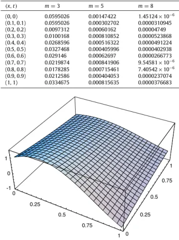
Table 1 Absolute error ofu

(

x

,

t

)

.

(

x

,

t

)

m

=

3 m

=

5 m

=

8 (0, 0) 0.0595026 0.00147422 1

.

45124

×

10−6 (0.1, 0.1) 0.0595026 0.000302702 0.0000310945 (0.2, 0.2) 0.0097312 0.00060162 0.00004749 (0.3, 0.3) 0.0100168 0.000810852 0.0000523868 (0.4, 0.4) 0.0268596 0.000516322 0.0000491224 (0.5, 0.5) 0.0327468 0.000405996 0.0000402938 (0.6, 0.6) 0.029146 0.00062697 0.0000266773 (0.7, 0.7) 0.0219874 0.000841906 9

.

54581

×

10−6 (0.8, 0.8) 0.0178285 0.000715461 7

.

40542

×

10−6 (0.9, 0.9) 0.0212586 0.000404053 0.0000237074 (1, 1) 0.0334675 0.000815635 0.0000376683

Fig. 1. Estimated and exact solutions ofu

(

x

,

t

)

.

4. Illustrative examples

To demonstrate the applications of the new method described in the current paper and its performance, the results

obtained for several examples [

3

,

4

,

1

,

17

,

18

] are presented in this section.

Example 1.

Consider Eqs.

(1)–(4)

with

ρ(

x

)

=

2 sin

(π

x

),

ψ(

x

)

= −

2 cos

(π

x

),

f

(

x

)

=

sin

(π

x

)

+

cos

(π

x

),

Q

(

x

,

t

)

=

(π

2

−

1

)

e

−t

(

sin

(π

x

)

+

cos

(π

x

)),

which has the exact solution

u

(

x

,

t

)

=

e

−t

(

sin

(π

x

)

+

cos

(π

x

)).

We plot the estimated and exact solutions in

Fig. 1

and present the absolute error

u

(

x

,

t

)

for some points in

Table 1

.

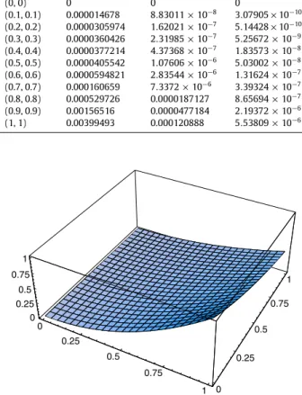
Example 2.

Consider Eqs.

(1)–(4)

with

ρ(

x

)

=

0

,

ψ(

x

)

=

3

,

f

(

x

)

=

x

2

,

Q

(

x

,

t

)

= −

(

2

+

x

2

)

e

−t

,

(8)

(

x

,

t

)

.

(

x

,

t

)

m

=

3 m

=

5 m

=

7 (0, 0) 0 0 0 (0.1, 0.1) 0.000014678 8

.

83011

×

10−8 ₃

.

₀₇₉₀₅

×

₁₀−10 (0.2, 0.2) 0.0000305974 1

.

62021

×

10−7 ₅

.

₁₄₄₂₈

×

₁₀−10 (0.3, 0.3) 0.0000360426 2

.

31985

×

10−7 ₅

.

₂₅₆₇₂

×

₁₀−9 (0.4, 0.4) 0.0000377214 4

.

37368

×

10−7 ₁

.

₈₃₅₇₃

×

₁₀−8 (0.5, 0.5) 0.0000405542 1

.

07606

×

10−6 ₅

.

₀₃₀₀₂

×

₁₀−8 (0.6, 0.6) 0.0000594821 2

.

83544

×

10−6 ₁

.

₃₁₆₂₄

×

₁₀−7 (0.7, 0.7) 0.000160659 7

.

3372

×

10−6 ₃

.

₃₉₃₂₄

×

₁₀−7 (0.8, 0.8) 0.000529726 0.0000187127 8

.

65694

×

10−7 (0.9, 0.9) 0.00156516 0.0000477184 2

.

19372

×

10−6 (1, 1) 0.00399493 0.000120888 5

.

53809

×

10−6

(

x

,

t

)

.

We plot the estimated and exact solutions in

Fig. 2

and present the absolute error

u

(

x

,

t

)

for some points in

Table 2

.

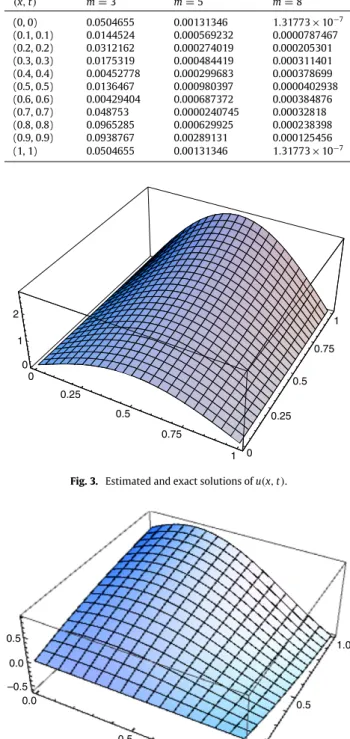
Example 3.

Consider the main partial differential equation such that

ρ(

x

)

=

0

,

ψ(

x

)

=

0

,

f

(

x

)

=

sin

(π

x

),

Q

(

x

,

t

)

=

(π

2

+

1

)

e

t

sin

(π

x

),

u

(

x

,

t

)

=

e

t

sin

(π

x

).

Fig. 3

u

(

x

,

t

)

for some points in

Table 3

.

Example 4.

Consider Eqs.

(1)–(4)

with [

30

]

ρ(

x

)

=

2 cos

(π

x

),

ψ(

x

)

= −

sin

(π

x

),

f

(

x

)

=

0

,

Q

(

x

,

t

)

=

(

sin

(π

x

)

+

cos

(π

x

))(

1

+

e

−t

+

π

2

(

1

−

e

−t

)),

having the exact solution

u

(

x

,

t

)

=

(

sin

(π

x

)

+

cos

(π

x

))(

1

−

e

−t

).

Fig. 4

u

(

x

,

t

)

with

m

=

8 and the absolute error

(9)

(

x

,

t

)

.

(

x

,

t

)

m

=

3 m

=

5 m

=

8 (0, 0) 0.0504655 0.00131346 1

.

31773

×

10−7 (0.1, 0.1) 0.0144524 0.000569232 0.0000787467 (0.2, 0.2) 0.0312162 0.000274019 0.000205301 (0.3, 0.3) 0.0175319 0.000484419 0.000311401 (0.4, 0.4) 0.00452778 0.000299683 0.000378699 (0.5, 0.5) 0.0136467 0.000980397 0.0000402938 (0.6, 0.6) 0.00429404 0.000687372 0.000384876 (0.7, 0.7) 0.048753 0.0000240745 0.00032818 (0.8, 0.8) 0.0965285 0.000629925 0.000238398 (0.9, 0.9) 0.0938767 0.00289131 0.000125456 (1, 1) 0.0504655 0.00131346 1

.

31773

×

10−7

(

x

,

t

)

.

(

x

,

t

)

.

Example 5.

Consider the parabolic partial differential equation [

52

] such that

ρ(

x

)

=

ψ(

x

)

= −

δ,

f

(

x

)

=

x

(

x

−

1

)

+

δ

6

(

1

+

δ)

,

(10)

Table 4

Absolute error ofu

(

x

,

t

)

.

(

x

,

t

)

Presented method withm

=

8 Method [30] (0.2, 0.1) 0.0000286444 6

.

6929

×

10−5 (0.5, 0.25) 0.0000300034 1

.

61436

×

10−4 (0.9, 0.45) 0.0000204942 2

.

37638

×

10−4 (0.1, 0.2) 0.0000354157 8

.

887543

×

10−5 (0.25, 0.25) 0.0000421702 1

.

44744

×

10−4 (0.45, 0.9) 0.0000377174 4

.

60293

×

10−5 (0.2, 0.2) 0.0000392584 1

.

00066

×

10−4 (0.4, 0.4) 0.0000405778 1

.

77034

×

10−4 (0.6, 0.6) 0.0000209623 1

.

77352

×

10−4 (0.8, 0.8) 6

.

67387

×

10−6 ₁

.

₀₀₂₄₇

×

₁₀−4 (0.9, 0.9) 0.0000205537 6

.

02934

×

10−4

(

x

,

t

)

.

Q

(

x

,

t

)

= −

e

−t

[

x

(

x

−

1

)

+

2

+

δ

6

(

1

+

δ)

]

,

which has the exact solution

u

(

x

,

t

)

=

e

−t

[

x

(

x

−

1

)

+

δ

6

(

1

+

δ)

]

, δ

=

0

.

0144

,

0

≤

x

≤

1

,

0

≤

t

≤

3

.

We first transfer 0

≤

t

≤

3 to

[

0

,

1

]

, so the equation is converted to

ρ(

x

)

=

ψ(

x

)

= −

δ,

f

(

x

)

=

x

(

x

−

1

)

+

δ

6

(

1

+

δ)

,

Q

(

x

,

t

)

= −

e

−3t

[

2

+

3



x

(

x

−

1

)

+

δ

6

(

1

+

δ)

]

,

with the exact solution

u

(

x

,

t

)

=

e

−3t

[

x

(

x

−

1

)

+

δ

6

(

1

+

δ)

]

, δ

=

0

.

0144

,

0

≤

x

≤

1

,

0

≤

t

≤

1

.

We plot the estimated and exact solutions of

u

(

x

,

t

)

in

Fig. 5

and present the absolute error for some points in

Table 5

.

5. Conclusion

In this paper the operational matrices for integration, differentiation, the product and the dual of Bernstein polynomials

basis are utilized to reduce solving the parabolic differential equation with nonlocal boundary conditions to the solution of

algebraic equations. The new method presented in the current paper can readily be extended to other appropriate parabolic

partial differential equations. The technique is general, easy to implement, and yields very accurate results. The numerical

(11)

Table 5

Absolute error ofu

(

x

,

t

)

.

(

x

,

t

)

Presented method withm

=

8

(0, 0) 3

.

4386

×

10−11 (0.1, 0.1) 0.0000171854 (0.2, 0.2) 0.0000454002 (0.3, 0.3) 0.0000690248 (0.4, 0.4) 0.0000840029 (0.5, 0.5) 0.0000894203 (0.6, 0.6) 0.0000853707 (0.7, 0.7) 0.0000725889 (0.8, 0.8) 0.0000525127 (0.9, 0.9) 0.0000272053 (1, 1) 8

.

20626

×

10−7

tests obtained by using the method developed in this article show that the new method produces acceptable results. Also

the presented upper bound of the error suggests convergence to the exact solution when

m

→ ∞

. It is worth noting

that the new technique developed in the current paper can be extended to solve similar problems in higher dimensions

[

48–51

,

19

].

Acknowledgments

The authors are very grateful to both reviewers for carefully reading the paper and for their comments and suggestions

which have led to improvement of the paper. Also we would like to thank the principal editor Professor Taketomo Mitsui

for managing the review process for this paper.

Appendix

Here, we describe how the smallness of the integral kernel in the nonlocal boundary condition affects the numerical

method. Therefore, we express some points as follows:

Definition 1.

Let

A

= [

a

i,j

]

(m+1)×(m+1)

and

B

= [

b

i,j

]

(m+1)×(m+1)

; we say that

A

≤

B

if only if

a

i,j

≤

b

i,j

for

i

,

j

=

1

,

2

, . . . ,

m

+

1.

Definition 2.

Function

G

(

x

,

t

)

∈

L

2

[

₀

,

1

]

is called small whenever



1 0



1 0

(

G

(

x

,

t

))

2

d

x

d

t

<

1

.

Proposition 1.

Let

φ

T

= [

B

0,m

,

B

1,m

, . . . ,

B

m,m

]

; then



1 0

φ(

t

)

T

d

t

=

1

m+1

[

1

,

1

, . . . ,

1

]

.

Also let Q be the operational matrix of

the dual; then the summation of elements of any column and any row of Q

−1

is m

+

1

.

Proof.

See [

47

].

It is clear that if function

G

(

x

,

t

)

is small then

G

(

x

,

t

)

is bounded, i.e.

∃

k

; ∀

(

x

,

t

)

∈ [

0

,

1

] × [

0

,

1

]

|

G

(

x

,

t

)

|

<

k

,

so the coefficient matrix

G

¯

= [ ¯

G

i,j

]

(m+1)×(m+1)

in the approximation

G

(

x

,

t

)

≃

φ(

x

)

T

G

¯

φ(

t

)

has bounded elements because

−

k

<

G

(

x

,

t

) <

k

H⇒ −

k

< φ(

x

)

T

G

¯

φ(

t

) <

k

⇒

−

k

φ(

x

)φ(

t

)

T

< φ(

x

)φ(

x

)

T

G

¯

φ(

t

)φ(

t

)

T

<

k

φ(

x

)φ(

t

)

T

⇒

−

k

∫

1 0

∫

1 0

φ(

x

)φ(

t

)

T

d

x

d

t

<

∫

1 0

∫

1 0

(φ(

x

)φ(

x

)

T

G

¯

φ(

t

)φ(

t

)

T

)

d

x

d

t

<

∫

1 0

∫

1 0

k

φ(

x

)φ(

t

)

T

d

x

d

t

.

Using

Proposition 1

we obtain

−

k

(

m

+

1

)

2

1

<

Q

¯

GQ

<

k

(

m

+

1

)

2

1

,

in which

1

is an

(

m

+

1

)

×

(

m

+

1

)

matrix whose elements are all 1. By multiplying both sides of this inequality by

Q

−1

and

employing

Proposition 1

we obtain

−

k1

<

G

¯

<

k1

,

so

−

k

<

G

¯

i,j

<

k

for

i

,

j

=

1

,

2

, . . . ,

m

+

1.

In this paper, we finally obtain a system of nonlinear algebraic equations. If the integral kernels are small then the

elements of the coefficient matrix of their approximations will be bounded, so the existing coefficient matrices in the system

of algebraic equations shrink and can be effectively solved, and thus the accuracy of the method increases.

(12)

References

[1] M. Dehghan, Efficient techniques for the second-order parabolic equation subject to nonlocal specifications, Appl. Num. Math. 25 (2005) 39–62. [2] S. Wang, Y. Lin, A numerical method for the diffusion equation with nonlocal boundary specifications, Int. J. Eng. Sci. 28 (1990) 543–546.

[3] M. Dehghan, A computational study of the one-dimensional parabolic equation subject to nonclassical boundary specifications, Numer. Methods Partial. Diff. Eqs. 22 (2006) 220–257.

[4] M. Dehghan, The one-dimensional heat equation subject to a boundary integral specification, Chaos Solitons Fractals 32 (2007) 661–675. [5] A. Bouziani, On a class of parabolic equations with a nonlocal boundary condition, Acad. Roy. Belg. Bull. Cl. Sci. 10 (1999) 61–77.

[6] A. Bouziani, Strong solution for a mixed problem with nonlocal condition for a certain pluriparabolic equations, Hiroshima Math. J. 27 (1997) 373–390. [7] J.R. Cannon, H.M. Yin, On a class of non-classical parabolic problems, J. Differential Equations 79 (1989) 266–288.

[8] A. Ashyralyev, A. Yurtsever, On a nonlocal boundary value problem for semilinear hyperbolic–parabolic equations, Nonlinear Anal. TMA 47 (2001) 3585–3592.

[9] J.R. Cannon, The One-Dimensional Heat Equation, in: Encyclopedia of Mathematics and its Applications, vol. 23, Addison-Wesley Publishing, Reading, MA, 1984.

[10] Y.S. Choi, K.Y. Chan, A parabolic equation with nonlocal boundary condition arising from electrochemistry, Nonlinear Anal. TMA 18 (1992) 317–331. [11] W.A. Day, Parabolic equations and thermodynamics, Quart. Appl. Math. 50 (1992) 523–533.

[12] W.A. Day, A decreasing property of solutions of a parabolic equation with applications to thermoelasticity and other theories, Quart. Appl. Math. 41 (1983) 468–475.

[13] W.A. Day, Heat Conduction within Linear Thermoelasticity, Springer, New York, 1985.

[14] A. Friedman, Monotonic decay of solutions of parabolic equation with nonlocal boundary conditions, Quart. Appl. Math. XLIX (1986) 468–475. [15] S. Mesloub, On a singular two dimensional nonlinear evolution equation with nonlocal conditions, Nonlinear Anal. TMA 68 (2008) 2594–2607. [16] M. Dehghan, Finite difference procedures for solving a problem arising in modeling and design of certain optoelectronic devices, Math. Comput.

Simulat. 71 (2006) 16–30.

[17] M. Dehghan, Numerical solution of a parabolic equation with non-local boundary specifications, Appl. Math. Comput. 145 (2003) 185–194. [18] M. Dehghan, Numerical solution of a parabolic equation subject to specification of energy, Appl. Math. Comput. 149 (2004) 31–45.

[19] M. Dehghan, Second-order schemes for a boundary value problem with Neumann’s boundary conditions, J. Comput. Appl. Math. 138 (2002) 173–184. [20] M. Dehghan, Numerical solution of a non-local boundary value problem with Neumann’s boundary conditions, Communications in Numerical Methods

in Engineering 19 (2003) 1–12.

[21] M. Tatari, M. Dehghan, On the solution of the non-local parabolic partial differential equations via radial basis functions, Appl. Math. Modelling 33 (2009) 1729–1738.

[22] M. Dehghan, A. Shokri, A numerical method for solution of the two-dimensional sine-Gordon equation using the radial basis functions, Math. Comput. Simulat. 79 (2008) 700–715.

[23] A. Bouziani, N. Merazga, S. Benamira, Galerkin method applied to a parabolic evolution problem with nonlocal boundary conditions, Nonlinear Analysis: TMA 69 (2008) 1515–1524.

[24] W.T. Ang, A method of solution for the one-dimensional heat equation subject to nonlocal conditions, SEA Bull. Math. 26 (2002) 197–203. [25] M. Dehghan, M. Ramezani, Composite spectral method for solution of the diffusion equation with specification of energy, Numer. Methods Partial

Diff. Eqs. 24 (2008) 950–959.

[26] A. Golbabai, M. Javidi, A numerical solution for non-classical parabolic problem based on Chebyshev spectral collocation method, Appl. Math. Comput. 190 (2007) 179–185.

[27] A.B. Gumel, On the numerical solution of the diffusion equation subject to the specification of mass, J. Aust. Math. Soc. Ser. B 40 (1999) 475–483. [28] Y. Liu, Numerical solution of the heat equation with nonlocal boundary conditions, J. Comput. Appl. Math. 110 (1999) 115–127.

[29] J. Martin-Vaquero, Two-level fourth-order explicit schemes for diffusion equations subject to boundary integral specifications, Chaos Solitons Fractals 42 (2009) 2364–2372.

[30] L. Mu, H. Du, The solution of a parabolic differential equation with non-local boundary conditions in the reproducing kernel space, Appl. Math. Comput. 202 (2008) 708–714.

[31] J. Qin, The new alternating direction implicit difference methods for solving three-dimensional parabolic equations, Appl. Math. Modelling 34 (2010) 890–897.

[32] A. Saadatmandi, M. Razzaghi, A Tau method approximation for the diffusion equation with nonlocal boundary conditions, Int. J. Comput. Math. 81 (2004) 1427–1432.

[33] Z.Z. Sun, A second-order accurate finite difference scheme for a class of nonlocal parabolic equations with natural boundary conditions, J. Comput. Appl. Math. 76 (1996) 137–146.

[34] Y. Zhou, M. Cui, Yingzhen Lin, Numerical algorithm for parabolic problems with non-classical conditions, J. Comput. Appl. Math. 30 (2009) 770–780. [35] M.I.M. Copetti, A one-dimensional thermoelastic problem with unilateral constraint, Math. Comput. Simul. 59 (2002) 361–376.

[36] J.H. Cushman, On diffusion in fractal porous media, Water Resour. Res. 27 (1991) 643–644.

[37] G. Dagan, The significance of heterogeneity of evolving scales to transport in porous formations, Water Resour. Res. 30 (1994) 3327–3336. [38] G. Ekolin, Finite difference methods for a nonlocal value problem for the heat equation, BIT 31 (1991) 245–255.

[39] J. Marti’n-Vaquero, J. Vigo-Aguiar, On the numerical solution of the heat conduction equations subject to nonlocal conditions, Appl. Numer. Math. 59 (2009) 2507–2514.

[40] C.V. Pao, Reaction diffusion equations with nonlocal boundary and nonlocal initial conditions, J. Math. Anal. Appl. 195 (1995) 702–718. [41] C.V. Pao, Numerical methods for nonlinear integro-parabolic equations of Fredholm type, Comput. Math. Appl. 41 (2001) 857–877.

[42] M. Dehghan, On the solution of an initial–boundary value problem that combines Neumann and integral condition for the wave equation, Numerical Methods for Partial Differential Equations 21 (2005) 24–40.

[43] F. Shakeri, M. Dehghan, The method of lines for solution of the one-dimensional wave equation subject to an integral conservation condition, Comput. Math. Appl. 56 (2008) 2175–2188.

[44] M.I. Bhatti, P. Bracken, Solutions of differential equations in a Bernstein polynomial basis, J. Comput. Appl. Math. 205 (2007) 272–280. [45] E. Kreyszig, Introductory Functional Analysis with Applications, John Wiley and sons. Inc., 1978.

[46] T.J. Rivlin, An Introduction to the Approximation of Functions, Dover Publications, 1981.

[47] S.A. Yousefi, M. Behroozifar, Operational matrices of Bernstein polynomials and their applications, Int. J. Syst. Sci 41 (2010) 709–716.

[48] M. Dehghan, M. Shamsi, Numerical solution of two-dimensional parabolic equation subject to nonstandard boundary specifications using the pseudospectral Legendre method, Numer. Methods Partial. Diff. Eqs. 22 (2006) 1255–1266.

[49] M. Dehghan, Fully explicit finite difference methods for two-dimensional diffusion with an integral condition, Nonlinear Analysis, Theory, Methods and Applications 48 (2002) 637–650.

[50] M. Dehghan, A new AD1 technique for two-dimensional parabolic equation with an integral condition, Comput. Math. Appl. 43 (2002) 1477–1488. [51] M. Dehghan, Numerical solution of the three-dimensional parabolic equation with an integral condition, Numerical Methods for Partial Differential

Equations 18 (2002) 193–202.

Journal of Computational and Applied Mathematics 235 (2011) 5272–5283

ScienceDirect