Effective and Efficient Optimization
Methods for Kernel Based Classification
Problems
byAditya Tayal
A thesis
presented to the University of Waterloo
in fulfilment of the
thesis requirement for the degree of
Doctor of Philosophy
in
Computer Science
Waterloo, Ontario, Canada, 2014
©Aditya Tayal 2014
Declaration
I hereby declare that I am the sole author of this thesis. This is a true copy of the thesis, including any required final revisions, as accepted by my examiners.
I understand that my thesis may be made electronically available to the public.
Aditya Tayal 2014
Abstract
Kernel methods are a popular choice in solving a number of problems in statistical machine learning. In this thesis, we propose new methods for two important kernel based classifica-tion problems: 1) learning from highly unbalanced large-scale datasets and 2) selecting a relevant subset of input features for a given kernel specification.
The first problem is known as the rare class problem, which is characterized by a highly skewed or unbalanced class distribution. Unbalanced datasets can introduce significant bias in standard classification methods. In addition, due to the increase of data in recent years, large datasets with millions of observations have become commonplace. We propose an approach to address both the problem of bias and computational complexity in rare class problems by optimizing area under the receiver operating characteristic curve and by using a rare class only kernel representation, respectively. We justify the proposed approach theo-retically and computationally. Theotheo-retically, we establish an upper bound on the difference between selecting a hypothesis from a reproducing kernel Hilbert space and a hypothesis space which can be represented using a subset of kernel functions. This bound shows that for a fixed number of kernel functions, it is optimal to first include functions corresponding to rare class samples. We also discuss the connection of a subset kernel representation with the Nyström method for a general class of regularized loss minimization methods. Com-putationally, we illustrate that the rare class representation produces statistically equivalent test error results on highly unbalanced datasets compared to using the full kernel repre-sentation, but with significantly better time and space complexity. Finally, we extend the method to rare class ordinal ranking, and apply it to a recent public competition problem in health informatics.
The second problem studied in the thesis is known as the feature selection problem in literature. Embedding feature selection in kernel classification leads to a non-convex optimization problem. We specify a primal formulation and solve the problem using a second-order trust region algorithm. To improve efficiency, we use the two-block
Gauss-Seidel method, breaking the problem into a convex support vector machine subproblem and a non-convex feature selection subproblem. We reduce possibility of saddle point convergence and improve solution quality by sharing an explicit functional margin variable between block iterates. We illustrate how our algorithm improves upon state-of-the-art methods.
Acknowlegements
I would like to thank my supervisors Professor Yuying Li and Professor Thomas Coleman for allowing me explore the field of machine learning and optimization. I have benefitted tremendously in both research and life skills during the course of my PhD years.
I thank my committee members, Stephen Wright (external), Mu Zhu, Peter Forsyth and Justin Wan, for taking the time to review the thesis and give me valuable comments. I would also like to thank fellow mates in the Scientific Computing lab, Kai Ma, Ken Chan, Eddie Cheung, Nick Nian, Haofan Zhang, Parsiad Azimzadeh and Swathi Amarala, for engaging and memorable discussions.
Contents
Contents vi List of Figures ix List of Tables x 1 Introduction 1 1.1 Contributions . . . 3 1.2 Outline . . . 5 2 Background 7 2.1 Support Vector Classification . . . 72.1.1 Linearly Separable Data . . . 7
2.1.2 Inseparable Data . . . 9
2.1.3 Dual Formulation . . . 10
2.2 Kernel Induced Feature Spaces . . . 11
2.2.1 Characterization . . . 14
2.2.2 Reproducing Kernel Hilbert Space (RKHS) . . . 15
2.3 Representer Theorem and Training in the Primal . . . 16
3 RankRC: Large-scale Nonlinear Rare Class Ranking 19 3.1 Introduction . . . 19
3.2 ROC Curve . . . 21
3.3 RankSVM . . . 24
3.4 RankRC: Ranking with Rare Class Representation . . . 26
3.5 Optimization Algorithm and Complexity . . . 29
Contents
3.5.2 Unconstrained Optimization . . . 30
3.6 Summary . . . 34
4 Theoretical Properties of RankRC 35 4.1 Comparison of RankRC with RankSVM . . . 36
4.1.1 Projected Mapping Equivalence . . . 36
4.1.2 Projected Mapping Bound . . . 41
4.2 Relation to Nyström Approximation . . . 46
4.2.1 Nyström Method Equivalence . . . 46
4.2.2 Nyström Approximation Bound for SVM . . . 48
4.2.3 Comparison to Kernel Perturbation Bounds . . . 50
4.3 Summary . . . 53
5 RankRC: Computational Results 55 5.1 Methods and Experiment Setup . . . 55
5.2 Simulated Data . . . 57
5.3 Real Datasets . . . 58
5.4 Intrusion Detection . . . 61
5.5 Summary . . . 67
6 Multi-Level Rare Class Kernel Ranking 68 6.1 Predicting Days in Hospital . . . 68
6.2 Ordinal Regression with Multi-Level RankRC . . . 69
6.3 Comparison of Results . . . 71
6.4 Summary . . . 73
7 Feature Selection 74 7.1 Introduction . . . 74
7.2 Feature Selection in Nonlinear SVMs . . . 77
7.2.1 Relation to GMKL . . . 79
7.3 Solving the Full-Space Feature Selection Problem . . . 80
7.3.1 Trust Region Algorithm . . . 81
7.4 Explicit Margin Sharing . . . 82
7.4.1 Simple AO . . . 82
Contents
7.4.3 Explicit (Functional) Margin AO-II . . . 89
7.5 Experiments . . . 91
7.5.1 Comparison to GMKL . . . 91
7.5.2 Feature Ranking Comparison . . . 97
7.6 Summary . . . 101
8 Conclusion 102 8.1 Future Work . . . 103
List of Figures
2.1 Example of linear discriminants separating two classes inR2 . . . 8
2.2 Convex loss functions and the smoothed hinge loss . . . 17
3.1 ROC analysis . . . 23
3.2 Example class conditional distributions for a rare class dataset . . . 28
4.1 Comparison of bounds for RankRC . . . 52
5.1 Example of simulated unbalanced dataset . . . 57
5.2 Comparison of ranking loss objective function . . . 60
5.3 Comparison of results for intrusion detection problem . . . 66
6.1 Output distribution for Heritage health provider problem . . . 69
6.2 Comparison of results for Heritage health provider problem . . . 72
7.1 2D example of NDCC simulated data . . . 92
7.2 Samples from FEI faces dataset . . . 94
7.3 Relevant features identifies for the FEI faces dataset . . . 95
7.4 Feature ranking results for NDCC . . . 98
7.5 Feature ranking results for FEI faces . . . 98
7.6 Feature ranking results for Sonar . . . 99
7.7 Feature ranking results for Ion . . . 99
7.8 Feature ranking results for S.A. Heart . . . 99
7.9 Feature ranking results for Musk . . . 99
7.10 Feature ranking results for Wdbc . . . 100
7.11 Feature ranking results for Aust. credit . . . 100
List of Tables
2.1 Examples of kernels . . . 13
3.1 Binary classification confusion matrix. . . 22
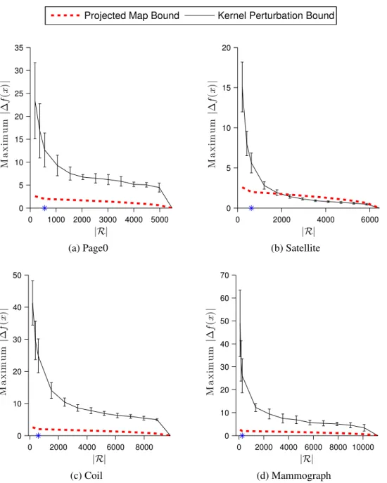
4.1 List of datasets used in bound comparison . . . 51
5.1 Comparison of test AUC results for simulated datasets . . . 59
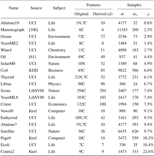
5.2 List of real unbalanced datasets . . . 62
5.3 Comparison of test AUC results for real datasets . . . 63
5.4 Comparison of number of support vectors for real datasets . . . 64
5.5 Intrusion detection output types . . . 65
7.1 Comparison of AO solution for feature selection . . . 84
7.2 NDCC dataset feature selection results . . . 93
7.3 Test results for FEI faces dataset . . . 94
Chapter 1
Introduction
Kernel methods are a popular choice in solving a number of problems in statistical ma-chine learning. The key benefit of kernel methods is separation of the training algorithm from data representation, encoded via a positive semi-definite kernel. Kernels allow us to estimate complex or nonlinear functions in a hypothesis space by implicitly estimating a linear model in a (usually high-dimensional) mapped space, known as the feature space. A kernel computes the dot product of two points in this feature space. Therefore, we can esti-mate linear models in the feature space without explicitly working in the high-dimensional space, as long as we can formulate the estimation process entirely in terms of dot products or kernel evaluations.
The model estimation process or learning algorithm can be decoupled from the specifics of the application area [35]. Domain knowledge or data structure for a particular application can be incorporated by choosing an appropriate kernel specification. For example, state-of-the-art vision classification systems often employ vocabulary-based representations, which can be effectively expressed via histogram kernels [5], or syntax based kernels can be defined over abstract structures, such as strings, trees or graphs [e.g. see 47, and references therein]. Thus a kernel can be used to capture salient features to represent the data space of a learning problem.
The learning algorithm is usually formulated as an optimization problem. Since the kernel is positive semi-definite, this often leads to a convex optimization problem—which has a unique minimum if it exists, and where any local minimum is also a global minimum. Thus the learning algorithm does not involve heuristic choices, such as learning rates or ini-tial points. Moreover, the same optimization algorithm can be used to solve problems with different kernel specifications. In this respect, kernel methods can be considered modular.
The theory of kernels is quite old, dating back to 1909 with Mercer [68]. The interpre-tation of kernels as dot products in a feature space was introduced into machine learning in 1964 by Aizerman et al. [7] on the method of potential functions. However, its possibilities were not fully understood until relatively recently by the introduction of the support vector machine by Boser et al. [15] in 1992.
By working implicitly in a high-dimensional feature space, kernels increase the risk of overfitting and ill-posedness of learning problems. That is, since the number of parameters is large compared to the number of training samples, a solution is likely to fit the training samples well, but have poor generalization performance on new unseen data. The statistical learning theory proposed by Vapnik and Chervonenkis [97] addresses this issue. In the context of a binary classification problem, they show that generalization error depends on the capacity of the hypothesis space, rather than the dimension of the problem, and that the capacity of linear discriminants can be controlled by maximizing the margin of the hyperplane with respect to training samples. Therefore kernels can safely be used to learn complex patterns with good generalization performance. The support vector machine (SVM) method employs this insight to learn a linear discriminant that maximizes margin while minimizing empirical error. Indeed, the success of SVMs in practical problems, backed by theoretical foundation, quickly led to its wide-spread popularity and revitalized interest in kernel methods.1
SVM model learning is formulated as a convex quadratic optimization problem with linear constraints. Traditionally, in the primal formulation, the problem is stated in terms of the parameters or weights of a linear discriminant function. The Lagrange dual formulation leads to a problem (and solution) that can be expressed entirely in terms of dot products, which can be replaced by kernel evaluations. This traditional perspective has led to the common misconception that in order to solve kernel SVMs one must resort to solving the dual optimization problem. However, recently Chapelle [25] shows that kernel SVMs can be solved using a primal formulation just as effectively.
In this thesis, we investigate two challenges associated with kernel based classification and illustrate how a primal approach can lead to effective and efficient solutions. The two problems are briefly described below. Background and relevant literature for each problem is reviewed in detail in Chapters 3 and 7, respectively, where they are introduced.
1Since Vapnik and Chervonenkis’ result, other generalization results based on Bayesian statistics,
com-pression schemes and stability analysis have also been posited to explain the performance of support vector machines and other kernel methods.
1.1 Contributions
1. Large-Scale Rare Class Learning:Rare class problems are characterized by highly unbalanced class distributions. Unbalanced datasets introduce significant bias in standard classification methods. Also, due to the increase of data in recent years, large datasets with millions of observations have become commonplace. We propose a primal solution to address both the problem of bias and computational complexity in rare class problems by optimizing area under the receiver operating characteristic curve and by using a rare class only kernel representation, respectively. We justify the approach theoretically and experimentally.
2. Feature Selection: Feature selection refers to the process of selecting an optimal subset of input features to improve generalization error and model interpretability, by discarding irrelevant or redundant inputs. We develop an embedded feature selec-tion method for kernel support vector machines based on a primal formulaselec-tion. We propose an effective and efficient solution to solve the resulting non-convex prob-lem using second-order optimization techniques and illustrate how our approach im-proves upon state-of-the-art methods.
1.1
Contributions
The contributions with respect to large-scale rare class learning are summarized below. 1. We propose to maximize area under curve (AUC) of the receiver operator
character-istic instead of minimizing empirical error in the support vector machine formulation for unbalanced problems. We argue that the AUC is a more appropriate empirical loss function for rare class problem than classification error. This results in a regular-ized biclass ranking problem, which is a special case of RankSVM [54]. RankSVM has generally been used in the context of ranking (e.g web page ranking) with linear models. Its application to nonlinear rare class learning has not been highlighted in previous literature.
2. To solve the dual optimization problem for kernel RankSVM requires O(m6) time and O(m4) space, where m is the number of data samples. Chapelle and Keerthi [26] show a primal approach can be used to solve RankSVM in O(m3) time and O(m2) space. We propose a modification to kernel RankSVM, that takes specific advantage of the unbalanced class distirbution, to achieveO(mm ) time andO(mm )
1.1 Contributions
space, wherem+ is the number of rare class examples. The idea is inspired by Zhu et al. [114], in which the posterior probability density is estimated with an adaptive bandwidth kernel density estimator over rare class samples and locally adjusted by the density of the background class. Using similar assumptions, we show the optimal solution can be approximately expressed as a linear combination of rare class kernel functions. In contrast to Zhu et al. [114], we use a regularized loss minimization approach to minimize a ranking loss objective while restricting the solution to a linear combination of rare class kernel evaluations. Additionally, in our method, the kernel does not need to be kernel density estimator, but can represent an arbitrary Mercer kernel. We call this method RankRC, since it enforces a Rare Class solution.
3. We view kernel RankRC as an approximation to kernel RankSVM, and mathemat-ically investigate the quality of approximation. Specifmathemat-ically, we establish an upper bound on the difference between the optimal hypotheses of RankSVM and RankRC. This bound is established by observing that any L2-regularized loss minimization problem, with a hypothesis restricted to an arbitrary subset of points, is equivalent to theL2-regularized loss minimization problem with a hypothesis instantiated by the full data set but using the orthogonal projection of the original feature mapping. 4. We show that the upper bound suggests that, under the assumption that a hypothesis
is instantiated by any subset of data points of a fixed cardinality, it is optimal to choose data points from the rare class first. Hence, this bound provides additional theoretical justification for RankRC.
5. We demonstrate that the Nyström kernel approximation method is equivalent to solv-ing a kernel regularized loss problem instantiated by a subset of data points corre-sponding to the selected columns. Consequently, theoretical bounds for Nyström kernel approximation methods can be established based on perturbation analysis of the orthogonal projection in the feature mapping. We demonstrate that this approach provides tighter bounds in comparison to established bounds based on the pertur-bation of the kernel matrix [32], which can be arbitrarily large depending on the condition number of the kernel approximation matrix.
6. We empirically compare RankRC to other methods on several datasets and illustrate predictive and computational advantages.
1.2 Outline
7. We extend the biclass RankRC formulation to multi-level ranking and apply it to a recent competition problem sponsored by the Heritage Health Provider Competition. The problem illustrates how RankRC can be used for ordinal regression where one ordinal level contains the vast majority of examples. We compare performance of RankRC with other methods and demonstrate computational and predictive advan-tages.
The contributions listed above also appear in Tayal et al. [90] and Tayal et al. [91]. The contributions with respect to feature selection are summarized below:
1. We invoke the Representer Theorem to formulate a primal embedded feature selec-tion SVM problem and use a smoothed hinge loss funcselec-tion to obtain a simpler bound constrained problem. We solve the resulting non-convex problem using a generalized trust-region algorithm for bound constrained minimization.
2. To improve efficiency we propose a two-block alternating optimization scheme, in which we iteratively solve (a) the standard SVM problem and (b) a smaller non-convex feature selection problem. Importantly, we propose a novel alternate opti-mization method by sharing a single perspective variable. We establish mathe-matical conditions under which this perspective variable sharing AO method avoids saddle points. For SVM feature selection, the perspective variable explicitly rep-resents the margin. We provide computational evidence to illustrate that this helps avoid suboptimal local solutions. Moreover, by focussing on maximizing margin in the feature selection problem—a critical quantity for generalization error—we are able to further improve solution quality.
3. We compare our methods to generalized multiple kernel learning and other leading nonlinear feature selectors, and show that our approach improves results.
The contributions to the feature selection problem also appear in Tayal et al. [92].
1.2
Outline
1.2 Outline
Chapter 3 introduces the RankRC model, Chapter 4 presents analytical results for RankRC, Chapter 5 shows the empirical results, and Chapter 6 extends the RankRC to multi-class ranking. Chapter 7 develops the primal feature selection method for kernel support vector machines. We conclude in Chapter 8 with summary remarks and potential extensions.
Chapter 2
Background
In this chapter, we briefly review support vector machines (SVMs), kernel induced feature spaces, and the primal optimization method for kernel SVM based on the Representer theo-rem. The chapter largely draws from material in Cristianini and Shawe-Taylor [35], Hastie et al. [52], Schölkopf et al. [82], Schölkopf and Smola [83], Vapnik [97].
2.1
Support Vector Classification
Support vector machines learn a linear discriminant rule (hyperplane) that separates two classes of data instances. This is known as the binary classification problem. Consider a set ofmtraining examples,D={(x1,y1),(x2,y2), ...,(xm,ym)}, wherexi∈ X ⊆Rdare data instances andyi∈ {+1,−1}are corresponding class labels (without loss of generality). We
seek a linear discriminant rule, f(x) =wTx+b, such that the class label of an observation
xis given byyˆi= sign(f(x)). In other words, we find a hyperplane ind-dimensional space,
wTx+b= 0, that separates the space into two half spaces, each corresponding to one of the
class labels.
2.1.1
Linearly Separable Data
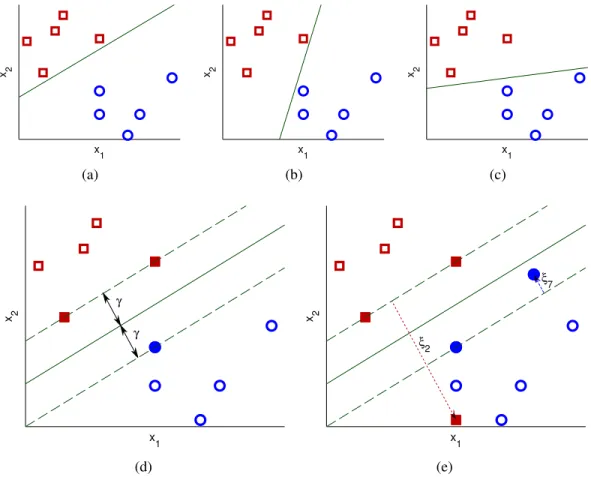
If the data is linearly separable, then there are an infinite number of linear discriminants that can separate the two classes (e.g see Figure 2.1a-c). According to the statistical learning theory of Vapnik [97], the optimal linear discriminant is the one that maximizes geometric margin between the two classes (Figure 2.1d), since it minimizes a bound on generalization error irrespective of the dimensionality of the space. Mathematically, this can be stated as a
2.1 Support Vector Classification x1 x 2 (a) x1 x 2 (b) x1 x2 (c) γ γ x1 x 2 (d) ξ 2 ξ 7 x1 x 2 (e)
Figure 2.1: Example dataset in (x1,x2)∈R2 space consisting of two classes with (red) squares representing one class and (blue) circles representing the other class. (a)-(c) In the separable case, there are many (infinite) linear discriminants which can separate the two classes perfectly. Three such discriminants are shown. (d) According to generalization bounds, the optimal linear discriminant is the one that maximizes the geometric margin,γ, between the two classes. (e) For inseparable or noisy datasets, we allow points to cross the margin, e.g.x2andx7, and penalize the violations,ξ2andξ7. In (d) and (e), support vectors
are shown as filled in circles.
convex optimization problem. Note, the hyperplane associated with (w,b) does not change upon rescaling to (λw,λb), for λ∈R+. The scaling affects the margin as measured by the function output as opposed to the geometric margin. The absolute value of function output at the closest point is called the functional margin. We can optimize the geometric margin by fixing the functional margin to 1 and minimizing the norm of the weight vector.
2.1 Support Vector Classification
Specifically, setting functional margin to 1 implies,
wTx++b= 1
wTx−+b=−1
wherex+ andx−are the closest points on the positive and negative sides of the hyperplane defined by (w,b). The geometric margin,γ, is then given by
γ= 1 2 wTx++b ∥w∥2 − wTx−+b ∥w∥2 = 1 2∥w∥2 (wTx++b)−(wTx−+b) = 1 ∥w∥2
Thus maximizing margin is equivalent to minimizing the norm of the weight vector. The convex optimization problem that solves for the maximum margin discriminant is,
min w,b 1 2∥w∥ 2 2 subject to yi wTxi+b ≥1, i= 1, ...,m,
where the constraint enforces a functional margin of 1 on both sides of the hyperplane.
2.1.2
Inseparable Data
Real data is often noisy and there may in general be no linear discriminant that can separate the data (see Figure 2.1e). To handle this case SVM uses penalized slack variables, ξi,i= 1, ...,m, which allow margin constraints to be violated:
min w,b,ξ 1 2∥w∥ 2 2+C m X i=1 ξi subject to yi wTxi+b≥1−ξi, i= 1, ...,m ξi≥0, i= 1, ...,m. (2.1)
Here,Cis a penalty parameter which balances the tradeoff between margin and violations. In practice, it is usually determined by cross-validation.
2.1 Support Vector Classification
2.1.3
Dual Formulation
We can transform Problem (2.1) into its corresponding Lagrange dual problem. Since the optimization problem is a convex quadratic programming problem, there is no duality gap. Therefore, an optimal solution of the primal problem is given by the dual problem. The dual formulations provides additional insight into the SVM problem. Also, it leads directly to a kernel approach to solve the problem in an implied feature space.
The Lagrangian for Problem (2.1) is L(w,b,ξ,α,r) = 1 2w Tw +C m X i=1 ξi− m X i=1 αi yi(wTxi+b)−1+xi − m X i=1 riξi,
withαi≥0 andri≥0 for dual feasibility. Stationarity implies,
∂L ∂w =w− m X i=1 yiαixi=0, ∂L ∂ξi =C−αi−r−i= 0, ∂L ∂b = m X i=1 yiαi= 0. Substituting these relations into the Lagrangian, we obtain the following dual objective function: L(w,b,ξ,α,r) = m X i=1 αi− 1 2 m X i,j=1 yiyjαiαjxTixj.
The constraint C−αi−ri= 0 together with ri ≥0 implies αi ≤C. Therefore, the dual optimization problem, which maximizesLor equivalently minimizes−L, is given by,
min α 1 2 m X i,j=1 yiyjαiαjxTi xj− m X i=1 αi subject to m X i=1 yiαi= 0 0≤αi≤C, i= 1, ...,m, (2.2)
where the constraints enforce stationarity conditions and dual feasibility. The Karush-Kuhn-Tucker (KKT) complementarity conditions provide useful information about the
2.2 Kernel Induced Feature Spaces
structure of the solution. These conditions state that a solution, (w∗,b∗,ξ∗,α∗) must satisfy,
α∗i yi(w∗Txi+b∗)−1+ξi∗ = 0, i= 1, ...,m ξi∗ α∗i −C= 0, i= 1, ...,m.
This implies a non-zero slack variable,ξi∗̸= 0, can only occur whenα∗i =C. These points are the margin violations, as their functional margin is less than 1, and their geometric margin is less than 1/∥w∥2. Points where 0<α∗i <Cimply,ξi∗= 0, andyi(w∗Txi+b∗) = 1. These points lie at the margin, with a geometric distance of 1/∥w∥2 from the hyperplane.
Points corresponding toα∗i = 0 lie beyond the margin in the correct half-space. From the first stationary condition, we havew=Pm
i=1yiαixi. Thus, the optimal hypoth-esis can be expressed in the dual representation as,
f(x) =w∗Tx+b=
m
X
i=1
yiα∗ixTi x+b∗. (2.3) The value ofb∗can be determined by solvingyif(xi) = 1 for anyiwith 0<α∗i <C, due to the complementarity conditions. Points corresponding to non-zero values ofα∗i are called support vectors, since in the expression (2.3) only these points are involved. Note, slight perturbations of points that are not support vectors will not affect the solution.
2.2
Kernel Induced Feature Spaces
So far we have considered linear hypothesis functions only. Real-world applications often require more expressive hypothesis spaces. That is, the target hypothesis function cannot be expressed as a simple linear combination of the input variables, but may require abstract features of the data to be exploited. For example, consider Newton’s law of gravitation as the target function, f(m1,m2,r) =Gm1m2/r2, in terms of massesm1,m2and distance,r. A
linear hypothesis in terms ofm1,m2,rcannot represent f, but a change of space obtained by mapping input features, (m1,m2,r)7→(x,y,z) = (lnm1,lnm2,lnr), gives the representation
g(x,y,z) = lnf(m1,m2,r) = lnC+lnm1,+lnm2−2 lnr=c+x+y−2z, which can be learned
using a linear function.
Kernels allow us to implicitly work in a high-dimensional derived feature space. The larger the set of mapped features, the more likely, the function to be learned can be
repre-2.2 Kernel Induced Feature Spaces
sented. Traditionally, a large number of derived features is known to degrade generalization performance, an effect popularly known as the curse of dimensionality. However, SVMs can avoid such degradation since generalization performance depends on the geometric margin of separation, and not the dimensionality of the feature space per se. Moreover, a large number of derived features would pose computational challenges, but since ker-nels bypass the need to compute the explicit feature map, high dimensional feature spaces (with even infinite dimensions) can be used, which otherwise would be computationally intractable.
Definition 1. Afeature map is a vector function,φ:X ⊆Rd→ F ⊆ Rd
′
, which maps the input spaceX to a derived feature space,F, i.e.
x= (x1, ...,xd)7→φ(x) = (φ1(x), ...,φd′(x)), whereF={φ(x)|x∈ X }.
A feature map is used to transform the data to a new space, in which a linear function is learned. The hypothesis space is f(x) =wTφ(x)+b, which can be a non-linear function
of the input featuresx.
Definition 2. Akernelis a function, k:X × X →R, such that for allu,v∈ X, k(u,v) =φ(u)Tφ(v),
whereφ:X → F is a feature map.
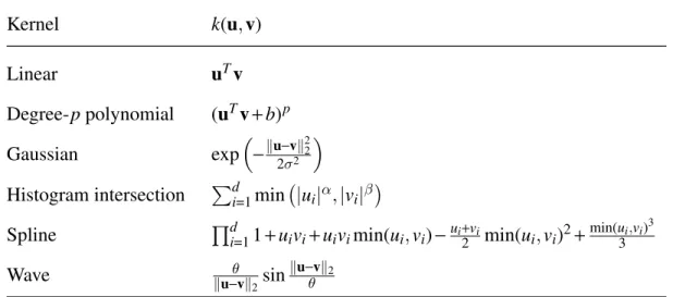
A kernel corresponds to the dot product in a derived feature space. In many cases, the dot product can be computed more efficiently using a simple function than by directly computing the dot product after explicitly forming the feature vectors. A few examples of common kernels are shown in Table 2.1.
Note, in the dual SVM problem (2.2) and the solution (2.3) all occurrences of data instances occur in a dot product. Therefore, we can replace these dot products with the kernel to implicitly compute the dot product in a derived feature space. This is known as
2.2 Kernel Induced Feature Spaces Kernel k(u,v) Linear uTv Degree-ppolynomial (uTv+b)p Gaussian exp −∥u−v∥ 2 2 2σ2 Histogram intersection Pd i=1min |ui|α,|vi|β Spline Qd
i=11+uivi+uivimin(ui,vi)−ui+2vimin(ui,vi)2+min(ui,vi)
3 3 Wave ∥uθ −v∥2sin ∥u−v∥2 θ
Table 2.1: Examples of kernels,k:Rd×Rd→
R. The Gaussian kernel is a popular non-linear kernel, often used as a default in absence of expert knowledge about the data. It corresponds to an infinite dimensional feature space and is in the class of universal kernels, i.e. it can approximate an arbitrary continuous target function uniformly, thereby minimiz-ing both estimation and approximation errors [70].
the “kernel trick”. The resulting problem is, min α 1 2 m X i,j=1 yiyjαiαjk(xi,xj)− m X i=1 αi subject to m X i=1 yiαi= 0 0≤αi≤C, i= 1, ...,m, (2.4)
with the solution,
f(x) = m
X
i=1
yiα∗ik(xi,x)+b∗. (2.5) The benefit of a kernel is that we do not need to know the underlying feature map in order to compute the dot product. A kernel is usually defined directly as a function, hence implicitly defining the feature space. This way we avoid the feature space not only in the computation of the dot product, but also in the design of the learning machine. The kernel can be viewed as a similarity measure between two points in the input space, X.
2.2 Kernel Induced Feature Spaces
Consequently, defining a kernel for an input space can be more natural than designing a complex feature space.
2.2.1
Characterization
Mercer’s condition [68] characterizes what constitutes a valid kernel according to Defini-tion 2. That is, Mercer’s theorem gives necessary and sufficient condiDefini-tions for a continuous symmetric functionkto admit an inner product representation in some feature space. We will not go into details of the analysis but simply quote the theorem below. In this thesis, we use the term kernel to refer to functions satisfying Mercer’s condition, though in the literature these are sometimes qualified as Mercer kernels.
Theorem 1. (Mercer) If k is a continuous kernel of a positive definite integral operator on L2(X), whereX is some compact space and L2(X)denotes the space of square-integrable functions, that is,
Z
X ×X
k(u,v)f(x)f(v)dxdv≥0,
for all f ∈L2(X), then it can be expanded as k(u,v) =
∞ X
i=1
λiφi(u)φi(v),
using eigenfunctionsφi∈L2(X)and eigenvaluesλi≥0.
In the dual SVM problem (2.4) we see the only information used is kernel evaluations on pairwise data in the training set. This can be stored in am×mmatrix, referred to as the kernel matrix.
Definition 3. Given a kernel k and inputs X ={x1, ...,xm} ∈ Xm, the m×m matrix K= [k(xi,xj)]mi,j=1 ,
is called thekernel matrix(orGram matrix) of the kernel k for the finite set X .
The conditions for Mercer’s theorem are equivalent to requiring that for any finite subset ofX, the corresponding kernel matrix is positive semi-definite [e.g. see 35] . This provides an alternative characterization of a kernel that is often more useful in practice.
2.2 Kernel Induced Feature Spaces
Proposition 2. Let X be a non-empty set with k:X × X →R a symmetric function on X. Then k is a Mercer kernel if and only if the kernel matrix K= [k(xi,xj)]mi,j=1is positive semi-definite (has non-negative eigenvalues) for all m∈N,xi∈ X,i= 1, ...,m.
2.2.2
Reproducing Kernel Hilbert Space (RKHS)
The feature map, φ, can also be defined as a map from X into the space of functions mappingX intoR, denoted asRX,
φ:X →RX , x7→φ k(·,x).
Here φ(x)(·) =k(·,x) represents the function that assigns the value k(x′,x) for any given pointx′∈ X.1 Following [83], we constructively build the Hilbert space of functions. This is done by defining a vector space of functions by taking linear combinations of the form
f(·) = m X i=1 aik(·,xi), g(·) = m′ X j=1 bjk(·,x′j), (2.6) wherem,m′∈N,a1, ...,am,b1, ...,bm′ ∈Randx1, ...,xm,x′1, ...,x′
m′ ∈ X are arbitrary. A dot product between f andgcan be defined as
⟨f,g⟩= m X i=1 m′ X j=1 aibjk(xi,x′j), (2.7)
which can be verified as a well-defined dot product on the vector space of functions given by (2.6). It can be verified that the dot product of f with the functionk(·,x) recovers f(x), i.e. ⟨f,k(·,x)⟩= f(x), which is known as the reproducing property of the kernel k. The space of functions (2.6) can be completed in the norm corresponding to the dot product (2.7) to obtain a Hilbert spaceH, called a reproducing kernel Hilbert space (RKHS). Thus, 1Note, viewingφ(x) as a function is compatible with the feature map perspective given in Definition
1, since a vector can represent coefficients of a function in a given feature space. For example, con-sider the feature mapφ:R27→R3 defined byx= [x1,x2]T 7→φ(x) = [x1,x2,x1x2]T, with kernelk(u,v) =
[u1,u2,u1u2][v1,v1,v1,v2]T. We can define a function of the features as f(x) =ax1+bx2+cx1x2, where
f :X =R2→R, and define an equivalent representation for f(·) = [a,b,c]T with f(x) = f(·)Tφ(x). The notation f(·) or simply f refers to the function itself, in the abstract, which may have multiple equivalent representations. Thus, whileφ(x) can be defined as a mapping fromR2toR3, it can also be seen to define the parameters of a function that mapsR2toR.
2.3 Representer Theorem and Training in the Primal
one can define a RKHS as a Hilbert spaceHof functions on a setX with the property that, for allx∈ X and f ∈ H, the point evaluations f 7→ f(x) are continuous linear functionals and all points f(x) are well defined. The Moore-Aronszajn theorem [8] states that for every Mercer kernel,k, there exists a unique RKHS and vice versa.
2.3
Representer Theorem and Training in the Primal
It is often presumed that to solve SVM with a kernel, we must solve the dual optimization problem (2.4). However, the primal SVM problem also admits the use of a kernel represen-tation. More generally, a large class of kernel problems can be written in the primal form using the Representer Theorem [82], without resorting to the dual optimization problem.
Theorem 3. (Representer Theorem) The solution to the following regularized loss mini-mization problem, min e f∈H h∈span{ψp} L(f(x1), ...,f(xm))+Ω(∥ef∥H), (2.8)
where f := ef+h,His a RKHS associated with kernel k, i.e.
H= ( e f ∈RX|ef(·) = ∞ X i=1 βik(·,zi),βi∈R,zi∈ X,∥ef∥H<∞ ) ,
{ψp}Mp=1is a set of M real-valued functions onX, with the property that the m×M matrix [ψp(xi)]ip has rank M, L:Rm→R∪ {∞}is an arbitrary cost function, andΩis a strictly monotonically increasing function on[0,∞], with∥fe∥2H=⟨ef,ef⟩defined by(2.7), admits a
representation of the form
f(·) = m X i=1 βik(·,xi)+ M X p=1 bpψp(·),
with unique coefficients bp∈R, for all p= 1, ...,M.
Note the hypothesis space in (2.8) also allowsMparametric basis functions on the input space, i.e.{ψp}Mp=1. This is useful, for example to include an offset term, as seen in SVM solution (2.5), i.e. settingM= 1 andψ1(x) = 1 for allx, impliesh∈R, which represents a scalar offset to ef.
2.3 Representer Theorem and Training in the Primal
The SVM problem (2.4) is a special case of (2.8), since it can be expressed in a primal exact-penalty form as:
min e f∈H b∈R C m X i=1 ℓh(yif(xi))+ 1 2∥ef∥ 2 H, (2.9)
where f(x) = ef(x)+b andℓh(z) = max(0,1−z) measures margin violations and is known
as the hinge loss function.2 From the Representer theorem we know the solution of (2.9) has the form f(x) =Pm
i=1βik(x,xi)+b, which also matches form (2.5) obtained using a
dual optimization argument. Finally, we can substitute this form in (2.9) to obtain a primal optimization problem in terms of the unknown model variables (β,b)∈Rm×
R.
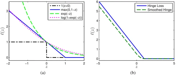
Apart from the hinge loss, other loss functions can also be used for classification pur-poses, for example see Figure 2.2a. According to the Representer Theorem, regardless of the loss function, the solution can be expressed in the form f(x) =Pm
i=1βik(x,xi)+b. Note, the loss functions are all convex approximations of the 0-1 loss function. The hinge-loss is robust to outliers and does not penalize correctly classified points, resulting in a sparse solution. Since the hinge-loss is non-differentiable, it can pose computational difficulties
2Consider replacing f(x)≡wTx+bin (2.1), and eliminatingξ
i’s by incorporating the constraint directly into the objective as a loss function.
−2 −1 0 1 2 0 1 2 3 z ℓ ( z ) 1(z<0) max(0,1−z) exp(−z) log(1+exp(−z)) (a) −5 0 5 0 1 2 3 4 5 6 z ℓ ( z ) Hinge Loss Smoothed Hinge (b)
Figure 2.2: (a) Shows different loss functions that are a convex approximation of 0-1 loss for classification problems. (b) The smoothed hinge is a differentiable approximation of the hinge loss. Here the smoothed hinge is shown withϵ= 0.5
2.3 Representer Theorem and Training in the Primal
in solving (2.9) using standard unconstrained optimization algorithms. Chapelle [25] pro-poses to use a differentiable approximation to the hinge loss (see Figure 2.2b),
ℓϵ(z) = (1−ϵ)−z ifz<1−2ϵ 1 4ϵ(1−z)2 if 1−2ϵ≤z<1 0 ifz≥1,
in place ofℓh, in (2.9) and uses Newton’s method to solve the resulting optimization prob-lem. Note, we can opt to use a twice-differentiable smoothed function as well, however in practice, this is not necessary since the overall objective is sufficiently smooth. From a classification perspective, the smoothed hinge loss function is margin-maximizing [79] and Bayes-risk consistent [72], and offers similar benefits as the hinge loss.
Chapter 3
RankRC: Large-scale Nonlinear Rare
Class Ranking
In this chapter, we introduce a new kernel based learning method for rare class problems called RankRC. Rare class problems are characterized by a highly unbalanced class distri-bution. In these situations, standard classification algorithms lead to biased models, since they focus on overall classification accuracy. In addition, many real-world rare class appli-cations involve large datasets, which are prohibitive for kernel methods.
RankRC addresses both the problem of bias and computational complexity for rare class problems by optimizing area under the receiver operating characteristic curve and by using a rare class only kernel representation, respectively. This chapter motivates and develops the problem formulation and optimization algorithm for RankRC.
3.1
Introduction
In many classification problems samples from one class are extremely rare (the minority class), while the number of samples belonging to the other class are plenty (the majority class). This situation is known as the rare class problem. It is also referred to as an unbal-anced or skewed class distribution problem. Rare class problems naturally arise in several application domains, for example, fraud detection, customer churn, intrusion detection, fault detection, credit default, insurance risk and medical diagnosis.
Standard classification methods perform poorly when dealing with unbalanced data, e.g. support vector machines (SVM) [55, 78, 107], decision trees [11, 29, 55, 102], neural
3.1 Introduction
networks [55], Bayesian networks [39], and nearest neighbor methods [11, 109]. Most classification algorithms are driven by accuracy (i.e. minimizing error). Since minority examples constitute a small proportion of the data, they have little impact on accuracy or total error. Thus majority examples overshadow the minority class, resulting in models that are heavily biased in recognizing the majority class. Implicitly, errors from different classes are assumed to have the same costs, which is usually not true. In most problems, incorrect classification of the rare class is more expensive, for instance, diagnosing a malignant tumor as benign has more severe consequences than the contrary case.
Solutions to the class imbalance problem have been proposed at both the data and algo-rithm level. At the data level, various resampling techniques are used to balance class dis-tribution, including random under-sampling of majority class instances [62], over-sampling minority class instances with new synthetic data generation [28], and focused resampling, in which samples are chosen based on additional criteria [109]. Although sampling ap-proaches have achieved success in some applications, they are known to have drawbacks, for instance under-sampling can eliminate useful information, while over-sampling can re-sult in overfitting. At the algorithm level, solutions are proposed by adjusting the algorithm itself. This usually involves adjusting the costs of the classes to counter the class imbalance [24, 65, 96] or adjusting the decision threshold [58]. However, true error costs are often unknown and using an inaccurate cost model can lead to additional bias.
We focus on nonlinear kernel based classification methods expressed as a regularized loss minimization problem. In recent years, we have also seen a rapid increase of data, resulting in many large scale rare class problems. For example, detecting unauthorized use of a credit card from millions of transactions. Processing large datasets can be prohibitive for many nonlinear kernel algorithms, which scale quadratically to cubically in the number of examples and may require quadratic space as well.
To address the challenges associated with rare class problems and large scale learning we propose the following:
1. Instead of maximizing accuracy (minimizing error), we optimize area under curve (AUC) of the receiver operator characteristic. The AUC overcomes inadequacies of accuracy for unbalanced problems and provides a skew independent measure. It is often used as the evaluation metric for unbalanced problems and therefore it is appropriate to directly optimize it in the training process. This results in a regularized biclass ranking problem, which is a special case of RankSVM with two ordinal levels [54].
3.2 ROC Curve
2. To solve a kernel RankSVM problem in the dual, as originally proposed in [54], requiresO(m6) time andO(m4) space, wheremis the number of data samples. Re-cently, Chapelle and Keerthi [26] proposed a primal approach to solve RankSVM, which results in O(m3) time and O(m2) space for nonlinear kernels. We propose a modification to kernel RankSVM, that takes specific advantage of the unbalanced nature of the problem, to achieveO(mm+) time andO(mm+) space, where m+ is the
number of rare class examples. The idea is inspired by Zhu et al. [114], in which the posterior probability density is estimated with an adaptive bandwidth kernel density estimator over rare class samples and locally adjusted by the density of the back-ground class. Using similar assumptions, we show the solution can be approximately expressed as a linear combination of rare class kernel functions. In contrast to Zhu et al. [114], we use a regularized loss minimization approach to minimize a ranking loss objective, but restrict the solution to a linear combination of rare class kernel evaluations. In our method, the kernel does not need to be kernel density estimator, but can represent an arbitrary Mercer kernel. We call this method RankRC, since it enforces a Rare Class solution.
In this chapter, we motivate RankRC assuming certain properties of the class distribu-tion and kernel choice. In Chapter 4 we analyze RankRC under general settings, and show that RankRC is optimal with respect to RankSVM for unbalanced datasets with a fixed cardinality of kernel functions.
The rest of the chapter is organized as follows. Sections 3.2 and 3.3 review the AUC measure and RankSVM. Section 3.4 develops the RankRC problem and presents justifica-tion for the rare class representajustifica-tion. Secjustifica-tion 3.5 outlines the optimizajustifica-tion algorithm used to solve RankRC.
3.2
ROC Curve
Evaluation metrics play an important role in learning algorithms. They provide ways to assess performance as well as guide modeling. For classification problems, error rate is the most commonly used metric. Consider the binary classification problem. Let D = {(x1,y1),(x2,y2), ...,(xm,ym)} be a set of m training examples, where xi∈ X ⊆ Rd, yi∈ {+1,−1}. Denote f(x) as the inductive hypothesis obtained by training on example setD.
3.2 ROC Curve
The empirical error rate is defined as,
ErrorRate= 1 m m X i=1 I[f(xi)̸=yi], (3.1) where I[p] denotes the indicator function and is equal to 1 if p is true, 0 if p is false. However, for highly unbalanced datasets, error rate is not appropriate since it can be biased toward the majority class [53, 66, 77, 86]. In this paper, we follow convention and set the minority class as positive and the majority class as negative. Consider a dataset that has 1 percent positive cases and 99 percent negative ones. A naive solution which assigns every example to be positive will obtain only 1 percent error rate. Indeed, classifiers that always predict the majority class can obtain lower error rates than those that predict both classes equally well. But clearly these are not useful hypotheses.
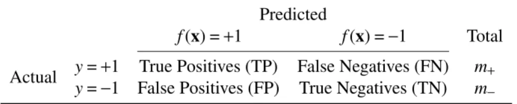
Classification performance can be represented by a confusion matrix as in Table 3.1, withm+ denoting the number of minority examples andm− the number of majority ones. The proportion of the two rows reflects class distribution and any performance measure that uses values from both rows will be sensitive to class skew.
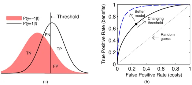
The Receiver Operating Characteristic (ROC) can be used to obtain a skew independent measure [19, 69, 77]. Most classifiers intrinsically output a numerical score and a predicted label is obtained by thresholding the score. For example, a threshold of zero leads to taking the sign of the numerical output as the label. Each threshold value generates a confusion matrix with different quantities of false positives and negatives (see Figure 3.1a). The ROC graph is obtained by plotting the true positive rate (number of true positives divided bym+) against the false positive rate (number of false positives divided by m−) as the threshold level is varied (see Figure 3.1b). It depicts the trade-off between benefits (true positive) and costs (false positives) for different choices of the threshold. Thus it does not depend on a priori knowledge of the costs associated with misclassification. A ROC curve that
Predicted
f(x) =+1 f(x) =−1 Total
Actual y=+1 True Positives (TP) False Negatives (FN) m+
y=−1 False Positives (FP) True Negatives (TN) m−
Table 3.1: Confusion matrix representing the results of a model for a binary classification problem.
3.2 ROC Curve TN FN TP FP ← Threshold P(y=−1|f) P(y=1|f) (a) 0 0.2 0.4 0.6 0.8 1 0 0.2 0.4 0.6 0.8 1
True Positive Rate (benefits)
False Positive Rate (costs) Better model Random guess Changing threshold (b)
Figure 3.1: ROC analysis. (a) Different quantities of True Positives (TP), False Positives (FP), False Negatives (FN) and True Negatives (TN) are obtained as the threshold value of a model is adjusted. (b) The ROC curve plots true positive rate against false positive rate for different threshold values. The dashed (blue) ROC curve dominates the solid (black) ROC curve. The dotted (gray) ROC curve has an AUC of 0.5, indicating a model with no discriminative value.
dominates another provides a better solution at any cost point.
To facilitate comparison, it is convenient to characterize ROC curves using a single measure. The area under a ROC curve (AUC) can be used for this purpose. It is the average performance of the model across all threshold levels and corresponds to the Wilcoxon rank statistic [51]. AUC represents the probability that the score generated by a classifier places a positive class sample above a negative class sample when the positive sample is randomly drawn from the positive class and the negative sample is randomly drawn from the negative class [37]. The AUC can be computed by forming the ROC curve and using the trapezoid rule to calculate the area under the curve. Also, given the intrinsic output of a hypothesis,
f(x), we can directly compute the AUC by counting pairwise correct rankings [37]:
AUC= 1 m+m− X {i:yi=+1} X {j:yj=−1} If(xi)≥ f(xj) . (3.2)
Incorporating the AUC in the modeling process leads to a biclass ranking problem, as discussed in the following section.
3.3 RankSVM
3.3
RankSVM
The modeling process can usually be expressed as an optimization problem involving a loss function and a penalty on complexity (e.g. regularization term). For most classification problems, since the performance measure is error rate, it is natural to consider minimizing the empirical error rate (3.1) as the loss function. In practice,I[·] is often replaced with a convex approximation such as the hinge loss, logistic loss or exponential loss [10]. Specif-ically, using the hinge loss, ℓh(z) = max(0,1−z), with ℓ2-regularization leads to the well
known support vector machine (SVM) formulation [15, 97], min w∈Rd 1 m m X i=1 ℓh yiwTxi +λ 2∥w∥ 2 2, (3.3)
whereλ∈R+is a penalty parameter that controls model complexity. Here, the hypothesis,
f(x) =wTx, is assumed linear in the input spaceX. Since SVMs try to minimize error rate, they can lead to ineffective class boundaries when dealing with highly skewed datasets, with resulting solutions biased toward the majority concept [107]. The literature contains several approaches to remedy this problem. Most prevalent are sampling methods and cost-sensitive learning. However, these approaches implicitly or explicitly fix the relative costs of misclassification. When the true costs are unknown, this can lead to suboptimal solutions.
Instead of minimizing error rate, we consider optimizing AUC as a natural way to deal with imbalance. Indeed, if we measure performance using AUC, it is preferable to optimize this quantity directly during the training process. In the AUC formula given in (3.2), we replaceI[·] with the hinge loss to obtain a convex ranking loss function. Thus we solve the following regularized loss minimization problem:
min w∈Rd 1 m+m− X {i:yi=+1} X {j:yj=−1} ℓh wTxi−wTxj +λ 2∥w∥ 2 2. (3.4)
Problem (3.4) is a special case of RankSVM proposed by Herbrich et al. [54] with two ordinal levels. Like SVM, RankSVM leads to a dual problem which can be expressed in terms of dot-products between input vectors. This allows us to obtain a non-linear function through the kernel trick [15], which consists of using a kernel function,k:X × X →R, that corresponds to a feature map,φ:X → F ⊆Rd′, such that∀u,v∈ X,k(u,v) =φ(u)Tφ(v). Here,kdirectly computes the inner product of two vectors in a potentially high-dimensional
3.3 RankSVM
feature space F, without the need to explicitly form the mapping. Consequently, we can replace all occurrences of the dot-product with kin the dual and work implicitly in space F.
However, since there is a Lagrange multiplier for each constraint associated with the hinge loss, the dual formulation leads to a problem inm+m−=O(m2) variables. Assuming
the optimization procedure has cubic complexity in the number of variables and quadratic space requirements, the complexity of the dual method becomes O(m6) time and O(m4) space, which is unreasonably large for even medium sized datasets.
As noted by Chapelle [25], Chapelle and Keerthi [26], we can also solve the primal problem in the implicit feature space due to the Representer Theorem [59, 82]. This the-orem states that the solution of any regularized loss minimization problem in F can be expressed as a linear combination of kernel functions evaluated at the training samples, k(xi,·),i= 1, ...,m. In the feature spaceF, problem (3.4) corresponds to solving
min w∈Rd′ 1 m+m− X {i:yi=+1} X {j:yj=−1} ℓh wTφ(xi)−wTφ(xj) +λ 2∥w∥ 2 2, (3.5)
where we have replacedxwithφ(x) and the hypothesis f(x) =wTφ(x), is a nonlinear func-tion of the input spaceX. Problem (3.5) cannot be solved directly, since the dimensional-ity,d′, of the feature space is usually very high (potentially infinite). Using the Representer Theorem, the solution of (3.5) in spaceF can be written as:
f(x) = m X i=1 βik(xi,x) = m X i=1 βiφ(xi)Tφ(x), orw= m X i=1 βiφ(xi). (3.6) By substituting (3.6) in (3.5) we can express the primal problem in terms ofβ:
min β∈Rm 1 m+m− X {i:yi=+1} X {j:yj=−1} ℓh m X r=1 βrk(xr,xi)− m X r=1 βrk(xr,xj) ! +λ 2 m X i,j=1 βiβjk(xi,xj),
3.4 RankRC: Ranking with Rare Class Representation or more simply, min β∈Rm 1 m+m− X {i:yi=+1} X {j:yj=−1} ℓh Ki
·
β−Kj·
β +λ 2β TK β, (3.7)whereK∈Rm×mis the kernel matrix,K
i j=k(xi,xj), andKi
·
denotes theith row ofK. To be able to solve (3.7) using unconstrained optimization methods such as gradient descent, we require the objective to be differentiable. We replace the hinge loss,ℓh, with anϵ-smoothed differentiable approximation,ℓϵ, defined as,ℓϵ(z) = (1−ϵ)−z ifz<1−2ϵ 1 4ϵ(1−z)2 if 1−2ϵ≤z<1 0 ifz≥1,
which transitions from linear cost to zero cost using a quadratic segment (see Figure 2.2b) and provides similar benefits as the hinge loss. Thus we can solve (3.7) using standard un-constrained optimization techniques. Since there aremvariables, Newton’s method would, for example, takeO(m3) operations to converge.
RankSVM is popular in the information retrieval community, where linear models are the norm [e.g. see 56]. For a linear model, withd-dimension input vectors, the complexity of RankSVM can be reduced toO(md+mlogm) [26]. However, many rare class problems
require a nonlinear function to achieve optimal results. Solving a nonlinear RankSVM requiresO(m3) time and O(m2) space [26], which is not practical for mid- to large-sized datasets. We believe this complexity is, in part, the reason why nonlinear RankSVMs are not commonly used to solve rare class problems.
In the next section we propose a modification to nonlinear RankSVMs that takes spe-cific advantage of unbalanced datasets to achieve O(mm+) time andO(mm+) space, while
not sacrificing predictive performance.
3.4
RankRC: Ranking with Rare Class Representation
To make RankSVM computationally feasible for large scale unbalanced problems, we pro-pose to enforce a rare class representation for the decision surface. Specifically, we propro-pose
3.4 RankRC: Ranking with Rare Class Representation
to restrict the solution to the form
f(x) = X
{i:yi=+1}
βik(xi,x), (3.8)
so it consists only of kernel function realizations of the minority class. We call this RankRC to indicate a Rare Class representation, instead of a support vector representation.
We present motivation for RankRC by assuming specific properties of the class condi-tional distributions and kernel function. Zhu et al. [114] make use of similar assumptions, however, in their method they attempt to directly estimate the likelihood ratio. In contrast, we are using a regularized loss minimization approach.
Recall that the optimal ranking function for a classification problem is the posterior probability,P(y= 1|x), since it minimizes the Bayes risk for arbitrary costs. From Bayes’ Theorem, we have
P(y= 1|x) = P(y= 1)P(x|y= 1)
P(y= 1)P(x|y= 1)+P(y=−1)P(x|y=−1). (3.9)
In addition, any monotonic transformation of (3.9) also yields equivalent ranking capability. Dividing the numerator and denominator of (3.9) by P(y=−1)P(x|y=−1), we note that
P(y= 1|x) is a monotonic transformation of the likelihood ratio, denoted as f(x) = P(x|y= 1)
P(x|y=−1) , (3.10)
which is the ranking function we are interested in obtaining.
Using kernel density estimation (also called the Parzen window estimate), the condi-tional densityP(x|y= 1) can be approximated using
P(x|y= 1) = 1 m+
X
{i:yi=+1}
aik(x,xi;σ) , (3.11)
where k(x,xi;σ) represents a kernel density function—typically a continuous unimodal function of xwith a peak at xiand a width localization parameter σ>0.1 The constants 1The kernel density function is not the same as a Mercer kernel described in Chapter 2. The kernel
density function used in the Parzen window estimate is a symmetric but not necessarily positive function that integrates to one. Mercer’s kernel described in Chapter 2 is associated with a unique Hilbert space of functions called its reproducing kernel Hilbert space (RKHS). It is more general in the sense that it can be
3.4 RankRC: Ranking with Rare Class Representation
x
P(x|y=−1)
P(x|y=1)
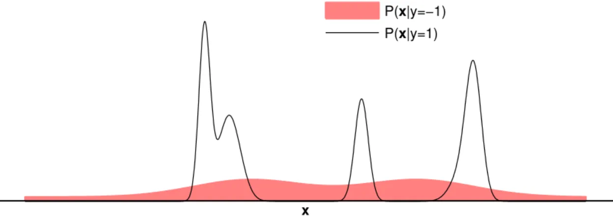
Figure 3.2: Example class conditional distributions for a rare class dataset showing that P(x|y= 1) is concentrated with bounded support, whileP(x|y=−1) is relatively constant in
the local regions around the positive class.
aiare used to normalize the density function and allow for a more general mixture model. For example, if we define
k(x,xi;σ) = exp
||
xi−x||2
σ2
as the Gaussian kernel, then (3.11) is equivalent to a mixture of m+ identical spherical normals centered at the rare class examples. This mixture model encompasses a large range of possible distributions to represent them+rare examples provided.
In rare class problems, most examples are from the majority class (y=−1) and only
a small number are from the rare class (y= 1). It is reasonable to assume the minority class examples are concentrated in local regions with bounded support, while the majority class acts as background noise. Therefore, in a neighborhood around the minority class examples, the conditional density functionP(x|y=−1) can be assumed to be relatively flat
in comparison toP(x|y= 1), see Figure 3.2 for instance. AssumeP(x|y=−1)≈cifor each minority examplei in the neighborhood ofxi.2 Together with (3.11), the likelihood ratio (3.10) can be written as
must be positive semi-definite (PSD). Ignoring normalization constants, well known examples of kernels that are both kernel density functions and Mercer kernels are the Gaussian kernel, multivariate Student kernel and the Laplacian kernel.
3.5 Optimization Algorithm and Complexity
f(x)≈ X
{i:yi=+1}
aik(xi,x)
ci , (3.12)
which only uses kernel functions at rare class points. The form (3.12) is equivalent to the rare class representation (3.8). In contrast to (3.6), this form takes specific advantage of the conditional density structure often found in rare class problems.
The rare class form (3.8) implies that
w= X
{i:yi=+1}
βiφ(xi). (3.13)
By substituting (3.13) in the regularized ranking loss problem (3.4), we obtain the following RankRC problem inm+ variables,
min β∈Rm+ 1 m+m− X {i:yi=+1} X {j:yj=−1} ℓh Ki+β−Kj+β +λ 2β TK ++β. (3.14)
Here,Ki+denotesith row ofKwith column entries corresponding to the positive class, and K++∈Rm+×m+is the square submatrix ofKcorresponding to positive class entries.
Although we motivated the rare class kernel formulation assuming certain properties of the class conditional distribution and kernel functions, we may still expect the rare class representation to perform adequately under more general settings. In Chapter 4 we shall analyze RankRC in a general setting, and show that for an unbalanced dataset, the rare class representation is optimal with respect to RankSVM when a fixed number of kernel functions are used. In the next section, we discuss the optimization method and algorithm complexity.
3.5
Optimization Algorithm and Complexity
As discussed earlier, we can replace the hinge loss, ℓh, with theϵ-smoothed differentiable approximation,ℓϵto obtain a differentiable objective function:
3.5 Optimization Algorithm and Complexity min β∈Rm+ 1 m+m− X {i:yi=+1} X {j:yj=−1} ℓϵ Ki+β−Kj+β +λ 2β TK ++β. (3.15)
To solve (3.15) we can use several approaches, which are discussed below.
3.5.1
Linearization
SinceK++ is a positive semi-definite matrix, it has an eigen-decomposition which can be expressed in the form,K++=UΛUT, withU being an orthogonal matrix (i.e.UTU=I) and
Λa diagonal matrix containing non-negative eigenvalues ofK++. Letw=Λ12UTβ, then
β=UΛ†12w, (3.16)
whereΛ† denotes the pseudoinverse ofΛ. We can substitute (3.16) in (3.15) to obtain the following linear (hypothesis) space problem,
min w∈Rm+ 1 m+m− X {i:yi=+1} X {j:yj=−1} ℓϵ Ki+UΛ†12w−K j+UΛ †1 2w +λ 2∥w∥ 2 2. (3.17)
That is, Problem (3.17) is equivalent to Problem (3.4) with data points given by xi = (Ki+UΛ† 1 2)T =Λ† 1 2UTKT i+∈R
m+,i= 1, ...,m. Therefore we can use the algorithm described
in Chapelle and Keerthi [26] to solve the linear ranking problem in O(mm++mlogm) =
O(mm+) time. The cost of computing xi=Ki+Uˆ
1
2,i= 1, ...,m, is O(mm2
+). The cost of
factoringK++ isO(m3+). Therefore the total time isO(mm2++m3+). Once we solve for
opti-malwwe can use (3.16) to obtainβ for subsequent testing purposes. Also, since we only need kernel entries{Ki j :yi= 1,j= 1, ...,m}, the method usesO(mm+) space.
3.5.2
Unconstrained Optimization
We can also directly solve (3.15) using standard unconstrained optimization methods. Gra-dient only methods, such as steepest descent and nonlinear conjugate graGra-dient do not re-quire estimation of the Hessian. Although this makes each iteration much cheaper, conver-gence can be slow, especially near the solution. In contrast Hessian based algorithms, such as Newton’s method can obtain quadratic convergence near the solution, but each iteration
3.5 Optimization Algorithm and Complexity
can be expensive. In Newton’s method, the pth iterate is updated according to
β(p+1)=β(p)
+s,
where the step,s, is obtained by minimizing the quadratic Taylor approximation around the current iterateβ(p): min s s Tg(p) +1 2s TH(p)s, (3.18) where H(p) and g(p) are the Hessian and gradient of the objective at β(p), respectively. Problem (3.18) has a closed form solution given by
s=−
H(p)
−1 g(p).
SinceH(p) is a m+×m+ matrix, this involvesO(m3+) cost in each iteration. To avoid this, we can use the truncated Newton method in which H(p)s=−g(p) is solved using linear
conjugate gradient. Here, the Hessian is not computed explicitly and the method iteratively approximates the solution using Hessian-vector products. Since each iteration in the linear conjugate gradient algorithm leads to a descent direction, we can terminate early while still improving convergence.
A drawback of (truncated) Newton’s method is that convergence can be guaranteed only from a certain neighbourhood of the solution. If the initial point is not chosen close enough to the solution, the method can be slow to converge, or fail altogether. Therefore we consider a subspace-trust-region method, which combines the benefit of a truncated Newton step with steepest descent. In our tests, we found that the subspace-trust-region method converges with significantly fewer iterations than the truncated Newton method.
The idea behind the trust-region method is to solve (3.18) while constraining the step,
s, to a neighborhood around the current iterate, in which the approximation is trusted: min s 1 2s TH(p)s +sTg(p) s.t. ||s||2≤∆(p). (3.19)
The trust region radius, ∆(p), is adjusted at each iterate according to standard rules, for example it is decreased if the solution obtained is worse than the current iterate. Problem
3.5 Optimization Algorithm and Complexity
(3.19) can be solved accurately [e.g see 18], however, the solution uses the full eigen-decomposition of H(p). To avoid this computation, in the subspace-trust-region method, Problem (3.19) is restricted to a two-dimensional subspace spanned by the gradient, g(p), and an approximate Newton direction,s2, which can be obtained by solvingH(p)s2=−g(p)
using linear conjugate gradient [21]. The idea behind this choice is to ensure global con-vergence, while maintaining fast local convergence. Once the subspace has been com-puted, solving (3.19) costs O(1) time, since in the subspace the problem is only two-dimensional. The implementation we use is provided in Matlab’s optimization toolbox,
fminunc/fmincon.
Computing Gradient and Hessian-Vector Product
We describe how we can compute the gradient and Hessian-vector product for Problem (3.15) efficiently. LetK
·
+ = [Ki j]i=1,...,m,yj=1∈Rm×m+ denote the rectangular submatrix of
Kwith columns indexed by the positive class. Consider the expanded matrix A= [Ki+−Kj+]i:yi=1,j:yj=−1∈Rm+m−×m+,
consisting of the differences of rows in K
·
+ corresponding to all pairwise preferences. In our computation we do not explicitly form matrixA, rather we note thatAcan be expressed as a sparse matrix product:A=PK
·
+,whereP∈Rm+m−×mis a sparse matrix that encodes a pairwise preference. That is, ify
i>yj, then there exists a rowr inPsuch thatPri = 1,Pr j=−1 and the rest of the row is zero. Let
Ar denote therth row ofA. Then the ranking loss expression in (3.15) can be written as,
X {i:yi=+1} X {j:yj=−1} ℓϵ Ki+β−Kj+β = m+m− X r=1 ℓϵ(Arβ) = m+m− X r=1 I[r∈ L] (1−ϵ−Arβ)+ m+m− X r=1 I[r∈ Q] 1 4ϵ(1−Arβ) 2 , (3.20)
whereL={r:Arβ<1−2ϵ}is the set of pairwise differences which are in the linear portion
3.5 Optimization Algorithm and Complexity
e∈Rm+m− as a vector of ones. DefineeL∈
Rm+m− as a binary vector whereeL
r = 1 ifr∈ L andeLr = 0 ifr̸∈ L. Also define IQ∈Rm+m−×m+m− as a diagonal matrix, whereIQ
rr = 1, if r∈ Q, andIrrQ= 0, ifr̸∈ Q. Then (3.20) is equivalent to
eLT((1−ϵ)e−Aβ)+ 1 4ϵ(e−Aβ) TIQ(e −Aβ) =eLT((1−ϵ)e−PK
·
+β)+ 1 4ϵ(e−PK·
+β) TIQ(e −PK·
+β) .Therefore the objective function in (3.15) can be expressed as
F(β), 1 m+m− eL T ((1−ϵ)e−PK
·
+β)+ 1 4ϵ(e−PK·
+β) TIQ(e −PK·
+β) +λ 2β TK ++β. (3.21) We obtain the gradient by taking the derivative of (3.21) with respect toβ:g, ∂F ∂β = 1 m+m− − eLTPK
·
++ 1 2ϵPK·
+I Q(PK·
+β−e) +λK++β = 1 m+m− − eLTP K·
++ 1 2ϵ PK·
+IQP(K·
+β) −P K·
+IQe +λK++β. (3.22) In the last expression we have used brackets to emphasize the order of operations that leads to an efficient implementation by avoiding the computation ofA=PK·
+. It can be verified that the time required isO(mm+).We obtain the Hessian by taking the derivative of (3.22) with respect toβ:
H , ∂ 2F ∂β∂βT = 1 2ϵm+m− PK
·
+IQPK·
+ +λK++.Note the Hessian requires computingA. However, for the linear conjugate gradient method we only require computingHsfor some vectors. In this case, we can avoid computingA by using the following order of operations:
Hs= 1 2ϵm+m− P K
·
+ IQP (K·
+s) +λK++s.The time required to computeHsis alsoO(mm+).
it-3.6 Summary
erations.3 We found the solution usually converges in a constant number of trust region iterations. Since each iteration requiresO(mm+) time, the total time required by the
algo-rithm isO(mm+). Total space is alsoO(mm+).
Finally, we note that we can slightly improve the time required to compute the gradient and Hessian-vector product by first sorting the values ofK
·
+β orK·
+s. Though this doesnot improve thebig-Oefficiency, it does reduce the constant factor. We refer the interested reader to [26] for details on a method which can be adapted for the nonlinear RankRC objective (3.15).
3.6
Summary
We use a ranking loss function to tackle the problem of learning from unbalanced datasets. Minimizing biclass ranking loss is equivalent to maximizing the AUC measure, which overcomes the inadequacies of accuracy, used by conventional classification algorithms. The resulting regularized loss minimization problem corresponds to a