Kernel-based expectile regression

Von der Fakult¨at Mathematik und Physik der Universit¨at Stuttgart zur Erlangung der W¨urde eines

Doktors der Naturwissenschaften (Dr. rer. nat.) genehmigte Abhandlung

Vorgelegt von Muhammad Farooq

aus Lahore, Pakistan

Hauptberichter: Mitberichter:

Tag der m¨undlichen Pr¨ufung:

Prof. Dr. Ingo Steinwart Prof. Dr. Andreas Christmann

13. Oktober 2017

Institut f¨ur Stochastik und Anwendungen der Universit¨at Stuttgart

Hiermit erkl¨are ich, dass ich die eingereichte Dissertation mit dem Titel Kernel-Based Expectile Regression

selbst¨andig angefertigt und keine anderen als die angegebenen Hilfsmittel benutzt habe. Alle Stellen, die dem Wortlaut oder dem Sinn nach anderen Werken, gegebenenfalls auch elektronis-chen Medien entnommen sind, sind von mir durch Angabe der Quelle als Entlehnung kenntlich gemacht.

. . . .

Ort, Datum Unterschrift

I express my deepest gratitude to my doctoral advisor Prof. Dr. Ingo Steinwart who gave me the opportunity to work with him in this research area. His continuous support and constructive discussion with him on the technical challenges during the journey of my Ph.D. always helped me to achieve my goals. He was also very supportive regarding non-technical issues. I could not have imagined having a better advisor for my Ph.D. research work. Besides my advisor, I warmly thank Prof. Dr. Andreas Christmann for his interest and willingness to be a co-examiner for my doctoral thesis.

I would like to thank all my old and new colleagues of ISA who made my stay in this institute memorable by giving me the opportunity of travelling with them and having fruitful discussions with them. Special thanks go to Dr. Philipp Thomann, Simon Fischer, Ingrid Blaschzyk and Thomas Hamm for reviewing my thesis and providing their valuable comments and suggestions in order to improve it. I would also like to thank Elke Maurer for helping me in many different ways throughout my journey.

With all my heart I express my deepest gratitude to my parents, the closest persons to whom this thesis is especially dedicated. They always let me go the way I like and encourage me to achieve my goals. Words cannot express the scarifies they have made in order to fulfill my dreams. Thank you from the bottom of my heart! I am also thankful to my sisters and brother. Their love, support, and prayers were always with me during this journey.

Abstract 1 Kurzfassung 3 Publications 5 Abbreviations 7 1 Introduction 9 2 Fundamentals 21

2.1 Some Properties of Losses and Their Risks . . . 21

2.2 Kernels and Reproducing Kernel Hilbert Spaces . . . 26

2.3 An Overview of the Statistical Analysis of SVMs . . . 29

2.4 Introduction to Convex Optimization . . . 34

3 Asymmetric Least Squares Loss: Self-Calibration and Variance Bounds 39 3.1 Loss Functions for Quantiles and Expectiles . . . 39

3.2 Properties of the Asymmetric Least Squares Loss . . . 42

3.2.1 Convexity . . . 42

3.2.2 Clipping . . . 42

3.2.3 Local Lipschitz Continuity . . . 43

3.2.4 Self-Calibration Inequalities . . . 44

3.2.5 Supremum and Variance Bounds . . . 49

4 Learning Rates for Kernel-Based Expectile Regression 51 4.1 Learning Rates Assuming Gaussian RBF Kernels . . . 53

4.1.1 Improved Entroy Bounds for the Gaussian RKHSs . . . 53

4.1.2 Approximation Error Bounds . . . 55 vii

viii

4.1.3 Learning Rates for Bounded Regression . . . 59

4.1.4 Learning Rates using Data Dependent Parameter Selction . . . 63

4.1.5 Learning Rates for Unbounded Noise . . . 66

4.2 Learning Rates Assuming Generic Kernels . . . 68

4.3 Conclusion . . . 73

5 An SVM-like Solver for Expectiles Regression 75 5.1 Primal and Dual Optimization Problem . . . 76

5.2 Working Set of Size One . . . 78

5.2.1 Stopping Criteria . . . 85

5.2.2 Initialization . . . 88

5.3 Working Set of Size Two . . . 90

5.3.1 Exact Solution of Two Dimensional Problem . . . 90

5.3.2 Working Set Selection Strategies . . . 97

5.3.3 Stopping Criteria . . . 98

5.4 Convergence Analysis . . . 98

5.5 Experiments . . . 104

Appendix A 113 A.1

Results for Different Working Set Selection Methods

A.2

Results for Different Number of Nearest Neighbors

A.3

Results for Different Initialization Methods

A.4

Results for Different Stopping Criteria

Bibliography 131

Conditional expectiles are becoming an increasingly important tool in finance as well as in other areas of application such as demography when the goal is to explore the conditional distribution beyond the conditional mean. In this thesis, we consider a support vector machine (SVM) type approach with the asymmetric least squares loss for estimating conditional expectiles. Firstly, we establish learning rates for this approach that are minimax optimal modulo a logarithmic factor if Gaussian RBF kernels are used and the desired expectile is smooth in a Besov sense. It turns out that our learning rates, as a special case, improve the best known rates for kernel-based least squares regression in aforementioned scenario. As key ingredients of our statistical analysis, we establish a general calibration inequality for the asymmetric least squares loss, a corresponding variance bound as well as an improved entropy number bound for Gaussian RBF kernels. Furthermore, we establish optimal learning rates in the case of a generic kernel under the assumption that the target function is in a real interpolation space.

Secondly, we complement the theoretical results of our SVM approach with the empirical findings. For this purpose we use a sequential minimal optimization method and design an SVM-like solver for expectile regression considering Gaussian RBF kernels. We conduct various experiments in order to investigate the behavior of the designed solver with respect to different combinations of initialization strategies, working set selection strategies, stopping criteria and number of nearest neighbors, and then look for the best combination of them. We further compare the results of our solver to the recent R-package ER-Boost and find that our solver exhibits a better test performance. In terms of training time, our solver is found to be more sensitive to the training set size and less sensitive to the dimensions of the data set, whereas, ER-Boost behaves the other way around. In addition, our solver is found to be faster than a similarly implemented solver for the quantile regression. Finally, we show the convergence of our designed solver.

Die Expectile Regression gewinnt im Finanzwesen, der Bev¨olkerungswissenschaft sowie in allen Anwendungsgebieten an Bedeutung, in denen detaillierten Eigenschaften als der Erwartungswert der bedingten Verteilung eine Rolle spielen. In dieser Arbeit betrachten wir einen Support Vec-tor Machine (SVM) Ansatz unter Verwendung der asymmetrischen Least-Squares Verlustfunk-tion zur Sch¨atzung der Expectiles einer bedingten Verteilung. Im ersten Abschnitt beweisen wir Lernraten f¨ur dieses Verfahren, welche bis auf einen logarithmischen Faktor minimax-optimal sind, falls wir den Gauß-Kern verwenden und die zu sch¨atzende Expectil-Funktion in einem gewissen Besov-Raum liegt. Als Spezialfall enth¨alt unsere Untersuchung die Least-Squares Regression und in diesem Fall liefert unser Beweis die bisher besten Raten f¨ur Gauß-Kerne. Unser Beweis st¨utzt sich in erster Linie auf eine allgemeine Kalibrierungsungleichung der asymmetrischen Least-Squares Verlustfunktion, einer zugeh¨origen Varianz-Schranke, sowie einer verbesserten Schranke an die Entropie-Zahlen des Gauß-Kerns. Desweiteren beweisen wir optimale Lernraten f¨ur beliebige Kerne unter der Annahme, dass die Expectil-Funktion in einem reellen Interpolationsraum liegt.

Im zweiten Abschnitt untermauern wir die theoretischen Resultate bzgl. unseres SVM-Ansatzes mit empirischen Untersuchungen. Dazu nutzen wir eine minimale sequentielle

Op-timierungsmethode, um einen Algorithmus zur Expectil-Regression bzgl. des Gauß-Kerns zu

entwickeln. Wir f¨uhren mehrere Expermimente durch, um das Verhalten unseres Algorithmuses unter verschiedenen Kombinationen von Initialisierungsstrategien, Auswahlstrategien, Stopp-kriterien und Anzahlen an Nearest Neighbors zu untersuchen. Ferner f¨uhren wir einen Vergleich zwischen unserem Algorithmus und dem R-package ER-Boost durch, in dem feststellen, dass unser Verfahren einen geringeren Testfehler aufweist. Die Trainingszeit unseres Algorithmuses h¨angt stark von der Gr¨oße des Trainingsdatensatzes ab, jedoch spielt die Dimension der Daten nur eine untergeordnete Rolle. Im Gegensatz dazu verh¨alt sich die Zeitkomplexit¨at des ER-Boost genau umgekehrt. Zus¨atzlich scheint es, dass unser Algorithmus schneller ist, als ein vergleichbarer Algorithmus zur Quantil-Regression. Abschließend beweisen wir die Konvergenz unseres Optimierungsverfahrens.

Some parts of this thesis have been published in:

• Learning Rates for Kernel-Based Expectile Regression

M. Farooq and I. Steinwart, Tech. Rep. 2017-003, Fakult¨at f¨ur Mathematik und Physik, Universit¨at Stuttgart, 2017. https://arxiv.org/abs/1702.07552

• An SVM-like Approach for Expectile Regression

M. Farooq and I. Steinwart, Comput. Stat. Data Anal., 109:159-181, 2017. https: //doi.org/10.1016/j.csda.2016.11.010

In addition, the source code of the solver for expectile regression (ex-svm) is now a part

of liquidSVM: A Fast and Versatile SVM Package. The package can be downloaded from

http://www.isa.uni-stuttgart.de/software/

ALS asymmetric least squares loss function

ALAD asymmetric least absolute deviation loss function SVM support vector machine

TV-SVM training-validation support vector machine RKHS reproducing kernel Hilbert space

RBF radial basis function

SMO sequential minimal optimization

i.i.d. independently and identically distributed

Introduction

Suppose that we have an input/output data setD:= ((x1, y1), . . . ,(xn, yn))∈(X×R)n drawn in an i.i.d. fashion from some unknown probability distribution P on X ×Y, where X is an arbitrary set and Y ⊂ _R. In addition, suppose that there exists a probabilistic relationship between input and output variables, that is, an input value x is drawn from the marginal dis-tribution PX of P on X and the corresponding output value y is drawn from the conditional

distribution P(Y|x), x ∈ X. Then, one of the goals of statistical learning is to estimate the characteristics of the conditional distribution P(· |x). For instance, one may be interested in estimating the central location measures of P(· |x), that one can estimate either by the con-ditional mean _E(· |x), x∈X using (non)parametric least squares regression or the conditional median med(· |x), x∈X with the help of (non)parametric median regression based on the least absolute deviation loss function. However, estimation of_E(·|x) or med(·|x) restricts us only to the central locations’ measures of the conditional distribution. In some real life applications, it is required to explore the conditional distribution P(· |x) beyond the center of the distribution. A wonderful remark in this regard is given by Mosteller and Tukey (1977):

“What regression curve does is give a grand summary for the average of the

dis-tribution corresponding to the set of xs. We could go further and compute several

different regression curves corresponding to the various percentage points of the dis-tributions and thus get a more complete picture of the set.”

One effort in this direction is made by Koenker and Bassett Jr (1978) by introducing the well-known quantile regression, a natural extension of the median regression, where the conditional quantiles of P(· |x) are obtained by minimizing the asymmetric least absolute deviation (ALAD) loss function. To be more precise, if P(· |x) has a strictly positive Lebesgue density, then the

10

τ-quantile qτ, τ ∈(0,1) of Y givenx∈X is a solution to

P(Y ≤qτ) =τ . (1.1)

For a detailed description, different estimation methods, and the theoretical analysis for the (conditional) quantile regression, we refer the reader to Koenker (2005), Takeuchi et al (2006), Christmann and Steinwart (2007), Steinwart and Christmann (2011), and references therein.

Another approach to characterize the conditional distribution is the expectile regression

proposed by Newey and Powell (1987). Let us denote by Q := P(Y|x) the conditional distri-bution of Y given x ∈X. In addition we assume that the first moment of Q is finite, that is,

|Q|1 := R

Y y dQ(y)<∞. Then the τ-expectile µ ∗ τ :=µ

∗

τ,Q∈ R for eachτ ∈(0,1) is the unique

solution of τ Z ∞ µ∗ τ (y−µ∗_τ)dQ(y) = (1−τ) Z µ∗_τ −∞ (µ∗_τ−y)dQ(y), (1.2) which is also strictly monotonically increasing for τ ∈(0,1), and continuously differentiable if the density ofQis continuously differentiable, see Newey and Powell (1987, Theorem 1). Unlike the quantiles that are determined by tail probabilities of Q, the expectiles are determined by the tail expectations.

One can estimate expectiles algorithmically by minimizing the expectation of a suitable loss function. There exists a class of loss functions that are consistent for expectiles. A general form of such class of loss functions can be found in Gneiting (2011, Theorem 10), see also Steinwart et al (2014, Equation (26)). However the only known convex loss function is the asymmetric

least squares loss (ALS) that has been considered in the literature extensively. For t ∈_R and

τ ∈(0,1), the ALS loss is defined by

Lτ(y, t) =      (1−τ)(y−t)2_{, if y < t ,} τ(y−t)2, if y_>t . (1.3)

Now using (1.3), the expectile µ∗_τ, τ ∈ (0,1) of the distribution Q, provided that the second moment of Q is finite, can be obtained by the optimization problem of the form

µ∗_τ := arg min

t∈R Ey∼Q

Lτ(y, t), (1.4)

see also e.g. Efron (1991) and Abdous and Remillard (1995) for further details.

Both quantiles and expectiles are special cases of so called M-quantiles as described by Breckling and Chambers (1988) and there exists a one-to-one mapping between them, see

e.g. Jones (1994) and Yao and Tong (1996). However, in general, expectiles do not coincide with quantiles of the same distribution. For instance, Jones (1994) showed that expectiles are in fact quantiles of some distribution related to the distribution of expectiles. Therefore, the choice between expectiles and quantiles mainly depends on the applications at hand, as it is the case in the duality between the mean and the median. For example, if the goal is to estimate a (conditional) threshold for which only a τ-fraction of (conditional) observations lie below this threshold, then a (conditional) τ-quantile is the right choice. On the other hand, if one is interested to estimate a (conditional) threshold for which the average distance of observation above this threshold is equal to the k times the average distance of observations below this threshold, then a τ-expectile regression is a preferable choice with k= 1−_ττ. Clearly, the focus in quantiles is ordering of the observations while expectiles account magnitude of the observations which makes expectiles sensitive to the extreme values of the distribution. Since expectiles estimation is computationally more efficient than quantiles estimation, one can use expectiles as a promising surrogate of quantiles in the situation where one is only interested in exploring the conditional distribution.

Expectiles have attracted considerable attention in recent years and have been applied successfully in many areas, for instance, in demography (see, Schnabel and Eilers, 2009a), in education (see, Sobotka et al, 2013) and extensively in finance, see for instance Wang et al (2011), Hamidi et al (2014), Xu et al (2016) and Kim and Lee (2016). In fact, it has recently been shown (see, e.g. Bellini et al, 2014; Steinwart et al, 2014) that expectiles are the only risk measures that enjoy the properties of coherence and elicitability, and therefore they have been suggested as potentially better alternative to the Value at Risk (VaR), see e.g. Taylor (2008), Ziegel (2016) and Bellini et al (2014). More importantly, for any τ ∈ (0,1), expectile immediately gives the realization of the gain-loss ratio or the Ω-ratio which is a well-known performance measure in portfolio management, see e.g. Keating and Shadwick (2002). For more applications of expectiles, we refer the interested readers to, e.g. Aragon et al (2005), Stahlschmidt et al (2014) and Guler et al (2014).

Recall (1.4) that the τ-expectiles can be computed with the help of asymmetric risks. To be more precise, for a measurable functionf :X →_R, the L-risk is defined by

RLτ,P(f) := Z X×Y Lτ(y, f(x))dP(x, y) = Z X Z Y Lτ(y, f(x))dP(y|x)dPX(x). (1.5)

Then there exists a PX-almost surely unique function fL∗τ,P :X →Rsuch that RLτ,P(f

∗

Lτ,P) =R ∗

12

provided that the second moment of P is finite, that is, |P|2 :=

ÄR

X×Y y2dP(x, y)

ä1/2

< ∞. Here, f_L∗

τ,P(x) is the optimal decision function that is often called the Bayes decision function,

and equals theτ-expectile of the conditional distribution P(· |x) for PX-almost allx∈X, that

isf_L∗_τ,P(x) =µ∗_τ,P(·|x)(x). A corresponding empirical estimator off_L∗_τ,Pis denoted byfD:X →_R

and can be obtained, for example, with the help of empirical Lτ-risks RLτ,D(f) = 1 n n X i=1 Lτ(yi, f(xi)). (1.6)

To obtain the empirical decision function fD, some semi-parametric and non-parametric

meth-ods have already been proposed in the literature . For instance, Schnabel and Eilers (2009b) considered penalized splines to compute smooth expectile estimates, Sobotka and Kneib (2012) proposed a couple of different procedures including least asymmetrically weighted squares in combination with mixed models, boosting within an empirical risk minimization framework, and a restricted expectiles regression model. Furthermore, a kernel method based on local lin-ear fits was considered by Yao and Tong (1996), and a boosting method using regression trees was proposed by Yang and Zou (2015).

Another class of non-parametric estimation methods, that we consider in this work, are the so-called kernel based regularized empirical risk minimizers, which include the well known

sup-port vector machines (SVMs), see Vapnik (2000, p. 138ff). Recall that SVMs build a predictor

fD,λ by solving an optimization problem of the form fD,λ = arg min

f∈Hλkfk 2

H +RL,D(f). (1.7)

Here,λ >0 is a regularization parameter,H is a reproducing kernel Hilbert space (RKHS) over

X with bounded, measurable kernelk, see e.g. Aronszajn (1950). These kernel-based methods often enjoy state-of-the-art empirical performance, relatively simple implementations, and a high flexibility. Their flexibility is based on two main ingredients, namely, the reproducing kernel Hilbert space (RKHS) H and the loss function L. The RKHS can be used to adapt to the nature of the input domainX, or more precisely, enables us to use both standard _Rd_-valued

data and non-standard data such as strings and graphs. Moreover, due to the so-called kernel-trick, the choice of H has little to no algorithmic consequences for solving SVM optimization problems. On the other hand, the choice of L determines the learning goal. For example, the so-called hinge loss is used for classification (Hush et al, 2006; Steinwart et al, 2011), the least squares loss leads to the conditional mean regression (Wu et al, 2006; Bauer et al, 2007; Caponnetto and De Vito, 2007; Steinwart et al, 2009; Eberts and Steinwart, 2013; Tacchetti

et al, 2013), and the ALAD loss is used to estimate conditional quantiles, see for example Steinwart and Christmann (2011) and Eberts and Steinwart (2013).

Having found an empirical estimator fD (or fD,λ in the case of (1.7)), its quality can be

measured by its distance to the target function f_L∗_τ,P, e.g. in terms of kfD−f_L∗_τ,PkL2(PX). For

estimators obtained by some empirical risk minimization scheme, however, one can hardly ever estimate this L2-norm directly, since f_L∗_τ,P and k · kL2(PX) are unknown. Instead, the standard

tools of statistical learning theory give bounds on the excess riskRLτ,P(fD)− R ∗

Lτ,P. Therefore,

our first goal in this thesis is to establish a so-called calibration inequality of Lτ that relates

both quantities. To be more precise, we will show in Theorem 3.3 that

C_τ−1(RLτ,P(f)− R ∗ Lτ,P)≤ kf −f ∗ Lτ,Pk 2 L2(PX) ≤c −1 τ (RLτ,P(f)− R ∗ Lτ,P), (1.8)

holds for all f ∈ L2(PX) and some constants cτ, Cτ only depending on τ. The right hand

side of (1.8) provides rates for kfD − fL∗τ,PkL2(PX) as soon as we have established rates for

RLτ,P(fD)− R

∗

Lτ,P. Furthermore, it is common knowledge in statistical learning theory that

bounds on RLτ,P(fD)− R ∗

Lτ,P can be improved if so-called variance bounds are available. We

will see in Lemma 3.4 that the right hand side of (1.8) leads to an optimal variance bound for

Lτ whenever Y is bounded. Note that both (1.8) and the variance bound are independent of

the considered expectile estimation method. In fact, both results are key ingredients for the statistical analysis of any expectile estimation method based on some form of empirical risk minimization. In addition, we will show in Lemma 4.12 that (1.8) leads to establish a bound for approximation error function in the case of generic kernels if the target function is in a real interpolation space, that is, f_L∗_τ,P ∈[L2(PX), H]β,∞for some β ∈(0,1), whereH is a RKHS for

a generic kernel.

Our second goal is to establish learning rates of the SVM-type algorithm (1.7). Since 2L1/2

equals the least squares loss, any statistical analysis of (1.7) also provides results for SVMs using the least squares loss. The latter have already been extensively investigated in the literature. For example, learning rates for generic kernels can be found in Cucker and Smale (2002), De Vito et al (2005), Caponnetto and De Vito (2007), Steinwart et al (2009), Mendelson and Neeman (2010) and references therein. Among these articles, only Cucker and Smale (2002), Steinwart et al (2009) and Mendelson and Neeman (2010) obtain learning rates in minimax sense under some specific assumptions. For example, Cucker and Smale (2002) assume that the target function f_L∗

1/2,P ∈ H, while Steinwart et al (2009) and Mendelson and Neeman (2010)

14

Recently Eberts and Steinwart (2013) have established (essentially) asymptotically optimal learning rates for least squares SVMs using Gaussian RBF kernels under the assumption that the target functionf_L∗

1/2,Pis contained in some Sobolev or Besov space. Recall that the Gaussian

RBF kernels are defined by

kγ(x, x0) := exp(−γ−2kx−x0k22), x, x

0 _∈

Rd,

whereγ >0 is called the width parameter that is usually determined in a data-dependent way, e.g. by cross-validation. A key ingredient of the work of Eberts and Steinwart (2013) is to control the capacity of RKHSHγ(X) for Gaussian RBF kernel kγ on the closed unit Euclidean

ball X ⊂_Rd _{by an entropy number bound}

ei(id :Hγ(X)→l∞(X))≤cp,d(X)γ −d

p i−

1

p, i≥1,

see Steinwart and Christmann (2008, Theorem 6.27), which holds for all γ ∈ (0,1] and all

p∈ (0,1]. Unfortunately, the constant cp,d(X) derived from Steinwart and Christmann (2008,

Theorem 6.27) depends on p in an unknown manner. As a consequence, Eberts and Steinwart (2013) were only able to show learning rates of the form

n−2α2α+d+ξ

for all ξ >0. To address this issue, we use (van der Vaart and van Zanten, 2009, Lemma 4.5) and derive the following improved entropy number bound

ei(id :Hγ(X)→l∞(X))≤(3K) 1 p Ç d+ 1 ep åd+1 p γ−dp_i− 1 p_{, i}≥_{1, (1.9)}

which holds for all p ∈ (0,1] and γ ∈ (0,1] and some constant K only depending on d. Note that (1.9) provides an upper bound for cp,d(X) whose dependence on p is explicitly known.

Using this new bound, we are then able to establish improved learning rates of the form (logn)d+1n−2α2α+d. (1.10)

Clearly these new rates replace the nuisance factornξ of learning rates of Eberts and Steinwart (2013) by some logarithmic term. Up to this logarithmic factor our new rates are minimax optimal (see Gy¨orfi et al, 2002, Chapter 1.7) iff_L∗_τ,P∈W₂α(_Rd) forα > ₂d or iff_L∗_τ,P∈B₂α_,∞(_Rd) for α > d. In addition, our statistical analysis provides learning rates for all asymmetric cases, that is, for τ 6= 1/2, which have not been established in the literature yet, and also were not possible to induce from the work of Eberts and Steinwart (2013).

Besides learning rates for the Gaussian RBF kernels (1.10), we also establish learning rates for generic kernels. For this we further assume that Y ⊂[−M, M], M >0 and that the target function is in a real interpolation space, i.e. f_L∗_τ,P ∈ [L2(PX), H]β,∞ for some β ∈(0,1), Then

we obtain optimal learning rates of the form

n−ββ+p_,

where p∈(0,1). For τ = 0.5, these rates are the same as the ones obtained by Steinwart et al (2009) in case of the least squares loss. However, the advantage with our rates is that they hold, modulo a constant term, for all τ ∈(0,1).

Our third goal in this thesis is to complement the above mentioned theoretical results of SVMs for Gaussian RBF kernels with the empirical findings. For this purpose, we design in the following an SVM-like solver for solving the optimization problem (1.7). Note that, besides Huang et al (2014) who have considered a kernelized iteratively reweighted strategy, no fully adaptive and efficient solver for the ALS loss has been proposed yet. For designing the solver, let us fix a feature space H0 and a feature map Φ :X →H0 of the considered kernel k. Then for all x∈X, one can represent f ∈H in terms ofw∈H0 via

f(x) =hw, φ(x)iH0, (1.11)

see Steinwart and Christmann (2008, Theorem 4.21) for further details. Note that the latter theorem also shows that

kfkH = inf{kwkH0 :w∈H0withf =hw, φ(·)iH0}. (1.12)

By using (1.6) together with (1.12) in (1.7), we then obtain the standard regularized problem for SVMs without offset

arg min w∈H0 λkwk2 H0 + 1 n n X i=1 Lτ(yi, f(xi)). (1.13)

About the last two decades the SVM-algorithmswithout offset have been considered because the offset term does in general not promise any theoretical and empirical advantages if one consider large RKHSs such as Gaussian RKHSs, see e.g. Vogt (2002), Steinwart (2003), Keerthi et al (2006), Steinwart et al (2011) and references theirin. On the contrary, the offset term imposes more restrictions on the solver. We will discuss on it in more details in Chapter 5.1. Now, we

16

reformulate (1.13) and obtain the primal optimization problem of the form arg min (w,ξ+,ξ−) w∈H PC(w, ξ+, ξ−) := 1 2kwk 2_+Cτ n X i=1 ξ_i,2₊+C(1−τ) n X i=1 ξ_i,2₋, such that ξi,+ ≥ yi − hw, φ(xi)i, ξi,− ≥ hw, φ(xi)i −yi, ξi,+ , ξi,− ≥0, ∀i= 1, . . . , n , (1.14)

where C := _2nλ1 > 0. Using standard Lagrangian techniques, one can easily obtain the dual optimization problem arg max (α,β) D(α, β) :=hα−β,yi − 1 2hα−β, K(α−β)i − 1 4Cτhα, αi − 1 4C(1−τ)hβ, βi, (1.15) αi ≥0, βi ≥0, ∀i= 1, . . . , n .

Hereyis then×1 vector of labels andK is then×nmatrix with entriesKi,j :=k(xi, xj), i, j =

1, . . . , n. The convexity of the loss (1.3) leads to the convexity of (1.14) which as a result leads to the concavity of (1.15). This ensures the fulfillment of the strong duality assumptions and consequently, the primal optimal solution can be obtained from a dual optimal solution using a simple transformation. To be more precise, if (α∗, β∗) is an optimal solution of the dual problem (1.15), then the optimal solution of the corresponding primal problem (1.14), for fixed

τ ∈(0,1), can be obtained by w∗ := n X i=1 (α∗_i −β_i∗)φ(xi), ξ_i,∗₊ := max ß 0, yi− hw∗, φ(xi)i ™ , ξ_i,∗₋ := max ß 0,hw∗, φ(xi)i −yi ™ , (1.16)

Moreover, we obtain for D∗ _:=D(α∗_{, β}∗_{) and P}∗ _:=P∗ C(w

∗_{, ξ}∗

+, ξ

∗

−) that D∗ =P∗. We further

obtain for fixedτ ∈(0,1) the following dual representation of the empirical conditional expectile estimator fD,λ defined by (1.7) fD,λ(·) = n X i=1 (α∗_i −β_i∗)k(·, xi). (1.17)

In order to achieve (1.17), we need to solve (1.15). Since (1.15) is of quadratic nature, we can implement quadratic programming (QP) techniques to solve (1.15). In the literature, we find many quadratic techniques for this purpose. However, in this thesis, we use the limiting case of decomposition method, namely, the Sequential Minimal Optimization (SMO) method

that optimizes two coordinates at each iteration (Platt, 1999). Note that the without-offset version of SVM allows us to design an SMO-type algorithm, namely, the 1D algorithm that can update one coordinate per iteration. For constants b1, b2 ∈(1,∞) and ci ∈ R, i ∈ {1, . . . , n},

we will show in Theorem 5.2 that this algorithm finds the 1D-feasible solution of (1.15) by using α+_i = max Å 0, ci b1 ã , β_i+= max Å 0,−ci b2 ã ,

where ci :=yi−Pnj6=i=1(αj −βj)k(xi, xj) and then chooses the best direction i∗ using the

1D-gain of the dual objective function. For constants b1, b2 ∈ (1,∞) and δ, η ∈R, the 1D-gain for

each i∈ {1, . . . , n} is obtained by G(δi, ηi) := δi Ç ∇Dαi(α, β)− b1δi 2 å +ηi Ç ∇Dβi(α, β)− b2ηi 2 å +δiηi,

whereδi =α+i −αi andηi =βi+−βi denote the difference between the new and the old values

of αi and βi respectively, and ∇Dαi(α, β) and∇Dβi(α, β) are the gradients of D(α, β) w.r.t. αi

and βi, respectively. Besides that, we establish a duality gap criterion to determine when 1D

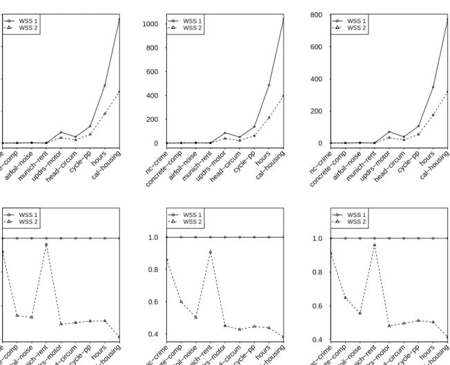
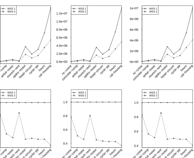
solver stops iterating. In addition, we design initialization strategies, namely, cold start and warm start, where the former initialize the solver with zeros and latter by recycling the old solution. Note that our designed SMO-type algorithm uses more than first order information, namely, the quadratic and concave nature of D(α, β) and exactly maximizing the gain in the dual during each iteration. Extending the idea of the 1D algorithm, we also design an SMO algorithm that updates two dual coordinates per iteration, see Section 5.3 for further details. In order to to obtain the optimal solution for (1.15), using only either the 1D algorithm above or a 2D algorithm that looks for the best pair of directions is not a suitable choice, because the former takes a longer time to converge and the latter requires a O(n2) search, see Steinwart et al (2011) in the case of the hinge loss. We therefore design two low-cost best direction search strategies, namely,WSS 1andWSS 2. The former searches for two 1D directions from two equal splits of the index set{1, . . . , n}, say i∗and j∗, respectively, for which the 1D-gain is maximum, and the latter first fix thei∗ chosen byWSS 1, and then searches for another directionj∗ based on the maximum 2D gain from k-nearest neighbors of xi with the metric d(x, x0) :=kx−x0k2.

We also show the theoretical convergence of our solver for expectile regression in Section 5.4. The behavior of the designed solver for the expectile regression is investigated by conducting various experiments. It turns out that the solver performs at its best when one chooses the warm start initialization method, theWSS 2working set selection strategy, the nearest neighbors size 15 and the duality gap without clipping as a stopping criterion. On the contrary, Steinwart

18

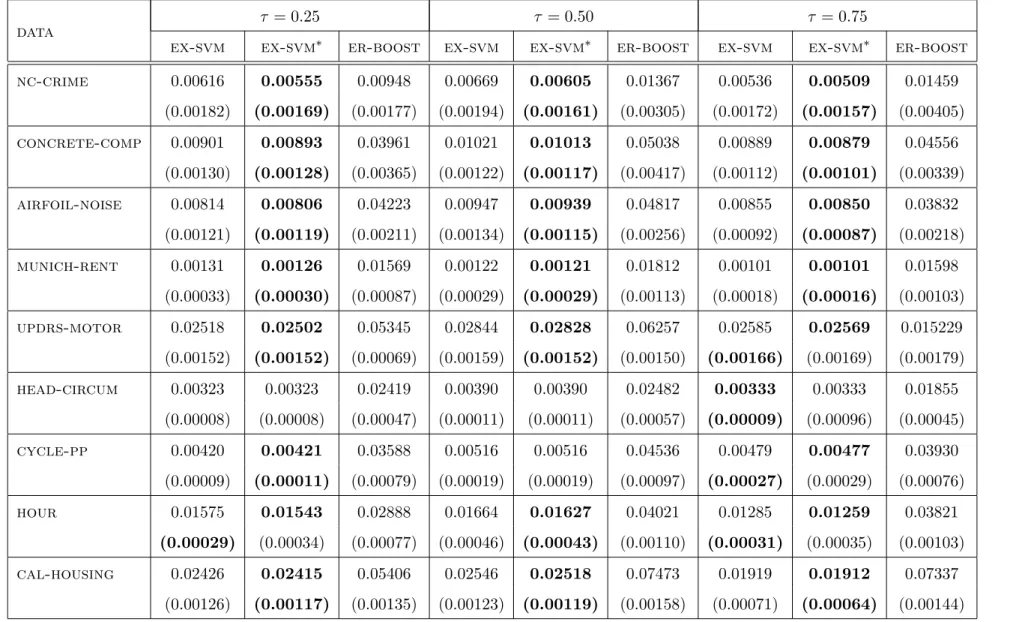
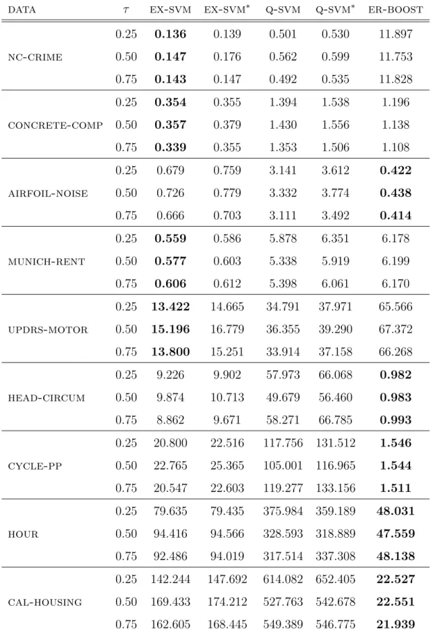
et al (2011) show that their solver for the hinge loss performs at its best when clipped duality gap is used as a stopping criterion with nearest neighbors size 10 while keeping the setting of aforementioned others criteria the same. We further compare the performance of our solver with respect to test error and training time to the R-package ER-Boost proposed by Yang and Zou (2015) for expectile regression. The results show, see Section 5.5, that the test performance of our solver is better thanER-Boost on various data sets. Regarding training time, we observe that our solver is more sensitive to the training set size and less sensitive to the dimensions of the data set, whereas, ER-Boost behaves the other way around. Finally, recall that one can use the expectiles as a computationally surrogate of the quantiles if one is interested only to explore the conditional distribution. We therefore compare the run times of our solver to the run time of the solver for quantile regression. It turns out the expectile solver is, depending on the data set size of the considered examples in Section 5.5, between 2 and 10 times faster than the solver for quantile regression, which shows the clear computational advantage of using expectile regression over quantile regression.

The rest of the thesis is organized as follows: Chapter 2 introduces some basic concepts, which include some properties of losses and their risks (Section 2.1), basics of kernels and their RKHSs (Section 2.2), a brief overview of the statistical analysis of SVMs (Section 2.3) and basic concepts of working with convex optimization problems (Section 2.4). In Chapter 3, we characterize the ALS loss function. Besides establishing Lipschitz continuity bounds for the ALS loss (Lemma 3.1), the so-called self-calibration inequalities (Theorem 3.3) are the main results of this chapter. These inequalities are then used to establish variance bounds in Lemma 3.4 for the ALS loss. The self-calibration inequalities and the corresponding variance bounds together with improved entropy bounds for Gaussian RKHSs (Lemma 4.2) are used as the key ingredients in Chapter 4 for establishing oracle inequalities (Theorem 4.6) and minimax optimal learning rates (Corollary 4.7) for SVMs under the assumption that Y ⊆ [−M, M],

M > 0 and the target function is smooth in a Besov sense (Section 4.1.3). In Section 4.1.4, we use a data-dependent parameter selection method that splits the data setD into a training and a validation set and achieves same learning rates adaptively, that is, without knowning the unknown smoothness parameters. Furthermore, we replace the assumption of bounded regression with the assumption of exponential decay of Y-tails in Section 4.1.5 and achieve the same learning rates. Finally, in Section 4.2, we consider generic kernels and obtain the learning rates under the assumption that Y ⊆ [−M, M] and that the target function is in a real interpolation space.

In Chapter 5 we design an SVM-like solver for expectile regression. This includes the formulation of the primal and the dual optimization problem for our learning scenario (Section 5.1), an algorithm for updating one coordinate along with some initialization strategies (Section 5.2) and an algorithm for updating two coordinates with some working set selection strategies (Section 5.3). In addition, the convergence analysis of the designed solver is given in Section 5.4. Finally, experimental results are presented in Section 5.5 where we investigate the behavior of the solver and compare its performance with the performance of existing R-package ER-Boost. The detailed results of the experiments are given in the appendix A.

In the end, we would like to mention that many of the results presented in this thesis have been published in advance. For instance, the results of Chapter 3 and partly of Chapter 4 have been published in Farooq and Steinwart (2017a). Moreover, the findings of Chapter 5 have been published in Farooq and Steinwart (2017b). Furthermore, the source code of the solver for expectile regression (ex-svm) has been added in the larger packageliquidSVM, see Steinwart and Thomann (2017), that can be downloaded from http://www.isa.uni-stuttgart.de/ software/.

Fundamentals

This chapter introduces some basic concepts which we use in the subsequent chapters. In Section 2.1 we present some notions of loss functions and their associated risks which will extensively be used in Chapter 3 to characterize the ALS loss function. Section 2.2 deals with basic concepts of kernels and their reproducing kernel Hilbert spaces. We also briefly describe the RKHSs of the well-known Gaussian RBF kernels that are often used in SVMs. After this, an overview of the statistical analysis of SVMs is given in Section 2.3. The concepts given in both Section 2.2 and Section 2.3 will be used in Chapter 4 in order to establish oracle inequalities and learning rates for the optimization problem (1.7). Finally, Section 2.4 covers the basics concepts of convex optimization that will be used in Chapter 5 to develop an algorithm using an SVM-like approach for solving (1.7). The contents of this chapter are primarily based on Cristianini and Shawe-Taylor (2000), Sch¨olkopf and Smola (2002), Boyd and Vandenberghe (2004), Abe (2005) and Steinwart and Christmann (2008).

2.1

Some Properties of Losses and Their Risks

Given an i.i.d. data set D := ((x1, y1), . . . ,(xn, yn)) ∈ (X ×Y)n drawn from some unknown

probability distribution P on X × Y, where X ⊂ _Rd _{and Y ⊂}

R, the goal of (supervised) statistical learning is to find a function f : X → _R such that for every pair (x, y)∈ (X×Y), the evaluation f(x) is a good prediction of the possible response y atx. In order to assess the quality of the “learned” function f, we recall some well established concepts from Steinwart and Christmann (2008, Chapter 2 and Chapter 3) and Sch¨olkopf and Smola (2002, Chapter 3). Let us begin by introducing the notion of loss function that measures the loss or cost of predicting response y at different levels of input variable(s).

22 2.1. Some Properties of Losses and Their Risks Definition 2.1 (cf. Steinwart and Christmann (2008, Definition 2.1)). Let (X,A) be a

mea-surable space and Y ⊂_R be a closed subset. Then a function L:X×Y ×_R→[0,∞) is called

a loss function if it is measurable.

We often use the notation L ◦f to represent the function (x, y) → L(x, y, f(x)). The loss function L can either be a supervised loss function defined by L := Y × _R → [0,∞) or an unsupervised loss function defined by L : X ×_R → [0,∞). In practice, the choice of loss function is determined by the learning problem at hand. For instance, in the case of the supervised loss, the classification loss Lclass :={−1,1} ×R →[0,∞) defined by Lclass(y, t) :=

1(−∞,0](ysignt) is used for the classification problem and theleast squares loss LLS :=Y ×R→

[0,∞) defined by LLS(y, t) := (y−t)2 is used for prediction. Furthermore, to study quantiles

and expectiles, the pin-ball loss and the asymmetric least squares loss are used respectively, see Steinwart and Christmann (2011) and Farooq and Steinwart (2017b) for further details. Note that a loss function can be characterized by its desirable properties. We define in the following the convexity and continuity of the loss function, see e.g. Steinwart and Christmann (2008, Definition 2.12 and 2.14), and we will further see in Chapter 5 that how the convex loss function leads to the convex optimization problem.

Definition 2.2 (cf. Steinwart and Christmann (2008, Definition 2.12 and 2.14)). A loss L :

X×Y ×_R→[0,∞) is called (strictly) convexand continuous if L(x, y,·) :_R→[0,∞)is

(strictly) convex and continuous, respectively, for all x∈X and y∈Y.

Recall Definition 2.1 that the loss function L measures only the loss of a function f for a fixed pair (x, y). In statistical learning, we are rather interested in theaverage loss, where the average is taken with respect to the probability distribution P.

Definition 2.3 (cf. Steinwart and Christmann (2008, Definition 2.2 and 2.3)). For a loss

function L :X×Y ×_R→ [0,∞) and a probability distribution P on X×Y, the L-risk of a

measurable function f :X →_R is defined by

RL,P(f) := Z X×Y L(x, y, f(x))dP(x, y) = Z X Z Y L(x, y, f(x))dP(y|x)dPX(x). (2.1)

Moreover, the minimal L-risk is defined by

R∗_L,P:= inf{RL,P(f)|f :X →R is measurable},

Here, the integral overX×Y always exists because (x, y)7→L(x, y, f(x)) is measurable and non-negative. If there exists a measurable functionf_L,∗_P:X →_Rsuch that RL,P(fL,∗P) =R

∗ L,P,

thenf_L,∗_P is called theBayes decision function (we will often call an optimal decision function). We will see in Chapter 3 in the case of the ALS loss that f_L,∗_P is unique, however, in some other cases it is not, see e.g. Steinwart and Christmann (2011) for the pinball loss.

The risk function RL,P(·) is measurable in the following scenario, see Steinwart and

Christ-mann (2008, Lemma 2.11) for proof. Assume that F ⊂ L0(X) := {f : X →R|fmeasurable}

is a subset equipped with a complete and separable metric d, and the corresponding Borel

σ-algebra. We also assume that lim

n→∞d(fn, f) = 0 =⇒ nlim→∞fn(x) =f(x), x∈X ,

for all fn, f ∈ F, that is d dominates the pointwise convergence. Then the map F ×X → R, (f, x)7→f(x) is measurable and thus are the mapX×Y×F →[0,∞), (x, y, f)7→L(x, y, f(x)) and the risk functional RL,P : F → [0,∞]. Here, it is interesting to note that the pointwise

convergence of the sequence of measurable functions (fn) to some f : X → R implies the

convergence of L(x, y, fn(x)) → L(x, y, f(x)) for all (x, y) ∈ X ×Y. However, this does not

generally hold for the convergence of associated risk RL,P(fn) to RL,P(f). In other words, the

risk of a continuous loss is not necessarily continuous. In that case, one can measure (local) Lipschitz continuity that holds for almost all frequently used loss functions.

Definition 2.4 (cf Steinwart and Christmann (2008, Definition 2.18)). A loss function L :

X×Y ×_R→[0,∞) is called

i) locally Lipschitz continuous if for all M >0, we have

|L|M,1 := sup t,t0_∈[−M,M] t6=t0 sup x∈X y∈Y L(x, y, t)−L(x, y, t0) |t−t0_| <∞.

ii) Lipschitz continuous if |L|1 := supM >0|L|M,1 <∞.

If Y ⊂_R is finite and L:Y ×_R→[0,∞) is a convex loss function, then by Steinwart and Christmann (2008, Lemma A.6.5), the loss L is locally Lipschitz continuous, and by Steinwart and Christmann (2008, Lemma 2.13 and Lemma 2.19), RL,P : L0(X) → [0,∞] is convex

and locally Lipschitz continuous, respectively. To be more precise, for all M > 0 and all

f, g ∈L∞(PX) withkfk∞≤M andkgk∞ ≤M, we have, see Steinwart and Christmann (2008,

Lemma 2.19)

24 2.1. Some Properties of Losses and Their Risks In the following, we present the notion of Nemitski loss.

Definition 2.5(cf. Steinwart and Christmann (2008, Definition 2.16)). A lossL:X×Y×_R→

[0,∞) is called a Nemitski loss if there exists a measurable function b:X×Y →[0,∞) and

an increasing function h: [0,∞)→[0,∞) such that

L(x, y, t)≤b(x, y) +h(|t|), (x, y, t)∈X×Y ×_R.

Furthermore, L is called a Nemitski loss of order p ∈ (0,∞), if there exists a constant

c >0 such that

L(x, y, t)≤b(x, y) +c|t|p_{, (x, y, t)∈X×Y ×}

R.

Finally, if P is a distribution on X×Y with b∈ L1(P), we say L is P-integrable Nemitski

loss.

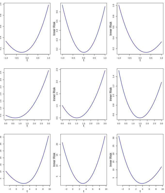
From Definition 2.3 it is trivial to see that the risk function (2.1) can be computed by iterated integrals. In other words, one can compute inner and outer integrals of (2.1) separately. This generates the idea of inner risks that are key ingredients of our analysis in Chapter 3.

Definition 2.6 (cf. Steinwart and Christmann (2008, Definition 3.3)). For a loss L:X×Y ×

R→[0,∞) and a distribution Q on Y, the inner L-risk of Q are defined by

CL,Q,x(t) := Z

Y

L(x, y, t)dQ(y), x∈X, t∈_R,

and the minimal inner L-risks are defined by

C_L,Q,x∗ := inf

t∈R

CL,Q,x(t), x∈X .

Given a distribution P on X×Y, the inner risks CL,P(·|x),x(f) of a function f can be used

to compute the risk RL,P(f) by

RL,P(f) = Z

X

CL,P(·|x),x(f(x))dPX(x).

Furthermore, Steinwart and Christmann (2008, Lemma 3.4 and Lemma 3.11) show that the minimal inner riskC∗

L,P(·|x),xis measurable inx∈Xand finite. Therefore,R ∗ L,Pcan be computed by R∗_L,P = Z X C_L,∗_P(·|x),xdPX(x).

In other words, the minimal riskR∗

L,Pcan be achieved bypointwisely minimizingthe inner risks CL,P(·|x),x, x ∈ X, which, in general, is easier than direct minimization of RL,P(·). Moreover,

one can compute the excess L-risk, when R∗

L,P<∞ holds, by RL,P(f)− R∗L,P=

Z

X

CL,P(·|x),x(f(x))− CL,∗P(·|x),xdPX(x), (2.2)

for all measurable f : X → _R. Clearly, one can obtain the excess risk first by analyzing the excess inner L-risks CL,P(·|x),x(f(x))− CL,∗ P(·|x),x, x ∈ X and then investigating the integration

with respect to PX, see Steinwart (2007). Besides some technical advantages, the analysis

only depends on P via the conditional distributions P(·|x) and hence allows us to consider the excess inner L-risks CL,Q,x(f(x))− CL,Q,x∗ for classes of distributions Q on Y as a template for CL,P(·|x),x(f(x))− CL,∗ P(·|x),x. This idea is very useful in the context of machine learning where we

assume that the distribution P and hence P(·|x), x∈X, is (almost) completely unknown, and the only information we have is that the distribution P belongs to a group of a certain type of distributions.

We conclude this section by presenting the idea of clipping that was first used by Bousquet and Elisseeff (2002) in the context of SVMs. Here we assume that Y ⊂ [−M, M] for some

M > 0, and we are interested in [−M, M]-valued estimator on X. For this, we need to restrict the loss Lto X×Y ×[−M, M].

Definition 2.7 (cf. Steinwart and Christmann (2008, Definition 2.22)). Let L:X×Y ×_R→

[0,∞) be a loss function and M > 0. Then we say that L can be clipped at M, if for all

(x, y, t)∈(X×Y ×_R) we have

L(x, y,Ût)≤L(x, y, t),

where Ût denotes the clipped value of t at ±M, that is

Û t:=              −M if t <−M , t if t∈[−M, M], M if t > M .

If L is a convex loss function, then by Steinwart and Christmann (2008, Lemma 2.23) L

can be clipped at M only ifY ⊆[−M, M] and Lhas at least one global minimizer in [−M, M]. In addition, the clipping operation potentially reduces the risks, that is, RL,P(fÛ) ≤ R_L,P(f).

We are therefore mostly interested in bounds of risk RL,P(fÛ) of the clipped decision function

rather than the risk RL,P(f) of the unclipped decision function. This also gives us algorithmic

advantages, see Steinwart et al (2011) and Chapter 5 for the case of the hinge loss and the ALS loss, respectively.

26 2.2. Kernels and Reproducing Kernel Hilbert Spaces

2.2

Kernels and Reproducing Kernel Hilbert Spaces

Reproducing kernels and their associated reproducing kernel Hilbert spaces (RKHS) are one of the main building blocks of SVMs, as we will see in Chapter 4 and Chapter 5. In this section, we present some basic notions of them. Let us first define kernels.

Definition 2.8 (c.f. Steinwart and Christmann (2008, Definition 4.1)). Let X be a non-empty

set. Then a function k :X×X →_R is called a kernel on X, if there exists a Hilbert Space H

and a map Φ :X →H such that, for all x, x0 ∈X, we have

k(x, x0) = hΦ(x),Φ(x0)iH, (2.3)

where Φ is called a feature map and H a feature space of k.

In general, the feature map Φ and the feature spaceH are not uniquely determined, however, different feature maps and corresponding feature spaces associated to the same kernel k lead to the unique inner product hΦ(x),Φ(x0)i. For instance, we have Φ1 and Φ2 that map into

feature spaces H1 and H2, respectively, associated to the same kernel k. If Φ1(x) 6= Φ2(x)

then consequently H1 6= H2, and furthermore spaces H1 and H2 may differ in terms of their

dimensions. However, we always havehΦ1(x),Φ1(x0)iH1 =hΦ2(x),Φ2(x

0_)i

H2. For further details

in this context, we refer the reader to Sch¨olkopf and Smola (2002, Chapter 2.2.2 and 2.2.4). Note that in case of high dimensional feature spaces, the computation of the inner product

hΦ(x),Φ(x0)iis expensive. However, for learning methods which only require the inner product of feature maps such as SVMs, the so calledkernel trick provides an alternative way to compute inner product without knowing the feature spaceH and without explicitly mapping intoH. In fact, the kernel trick makes it possible to compute the result of the inner product in the original space X implicitly, as we can see in the following examples of kernels. The detailed properties of these kernels can be found in Sch¨olkopf and Smola (2002, Chapter 2.3).

Example 2.9 (Polynomial Kernel). For m∈_N, c >0, and x, x0 ∈_Rd _{for d≥1, the kernel} k(x, x0) := (hx, x0i+c)m (2.4)

is called inhomogeneous polynomial kernel of order m. For c = 0, it is called homogeneous

polynomial kernel. Finally, for m = 1 and c= 0, it is called linear kernel.

Example 2.10 (Exponential Kernel). For d∈_N and x, x0 ∈_Rd_{, the kernel}

k(x, x0) := exp(hx, x0i), (2.5)

In Definition 2.8 the feature spaceH is required in order to decide whether a given function

k is a kernel, and this requirement sometimes becomes difficult to fulfill. In the following, we characterize kernels in terms of inequalities that helps to define kernels in a different way. Definition 2.11 (cf. Steinwart and Christmann (2008, Definition 4.15)). A function k : X×

X →_R is called positive definite if

n X

i,j=1

cicjk(xi, xj)≥0 (2.6)

holds for all n ∈ _N, c1, . . . , cn, and all x1, . . . , xn ∈ X. Moreover, k is said to be strictly

positive definite if, for mutually distinct x1, . . . , xn∈X, the equality in (2.6) only holds for

c1 =· · ·=cn = 0. Finally, k is called symmetric if k(x, x0) =k(x0, x) for all x, x0 ∈X.

In the latter definition, K := (k(xi, xj))i,j for all fixed x1. . . xn ∈ X is called the Gram

matrix, and (2.6) is equivalent to saying that Gram matrices are positive definite. The classical

and well-known result shows that the definiteness and symmetry of a function k are necessary and sufficient conditions to say that k is a kernel, see Steinwart and Christmann (2008, The-orem 4.16) for a proof. For more properties of kernel k, we refer the reader to Steinwart and Christmann (2008, Chapter 4.1).

In Definition 2.8, we note that the feature map Φ and the corresponding feature space H

are not uniquely determined. One way to resolve this problem is to choose a canonical feature map of the kernel k that leads to a well-known space called the reproducing kernel Hilbert space (RKHS). This space is the smallest feature space of the kernel k in a certain sense. Definition 2.12 (cf. Steinwart and Christmann (2008, Definition 4.18)). Let X 6=∅ and H be

a real-valued Hilbert function space over X.

i) A function k : X ×X → _R is called reproducing kernel of H if we have k(·, x) ∈ H

for all x∈X and if the reproducing property

f(x) = hf, k(·, x)i,

holds for all f ∈H and all x∈X.

ii) The space H is called a reproducing kernel Hilbert space over X if for all x ∈ X

the Dirac functional δx :H→R defined by

δx(f) := f(x),

28 2.2. Kernels and Reproducing Kernel Hilbert Spaces It is important to note that not every Hilbert space is RKHS but only those for which ii) holds, i.e, the Hilbert spaces in which the evaluation functionals are bounded. We further note that the reproducing kernelkis a kernel in the sense of (2.3) with feature spaceH and canonical feature map Φ :X →H (see Steinwart and Christmann, 2008, Lemma 4.19). It is also known, see Steinwart and Christmann (2008, Theorem 4.20, 4.21), that reproducing kernel of a RKHS is unique, and so is the RKHS associated to the positive definite kernel.

Another way of constructing RKHSs for a continuous positive definite kernel k is to choose Mercer maps that are combinations of eigenvalues-eigenfunctions of the integral operator Tk : L2(X) → L2(X). To be more precise, let k be a measurable and bounded kernel on X with

separable RKHS H and µ be a finite measure on X. Then the integral operator (Tkf)(·) :=

Z

X

k(·, x)f(x)dµ(x),

is compact, self-adjoint, and non-negative. Consequently, there exists an at most countable family of eigenvalues (λi)i∈I ⊂(0,∞) and corresponding orthonormal system (ONS) ([˜ei]∼)i∈I ⊂ L2(PX) of eigenfunctions of Tk. Moreover, we have Pi∈Iλi < ∞, and there exists a family

(ei)i∈I ∈H with

[ei]∼= [˜ei]∼ ∀i∈I

and a measure set N ∈X with PX(N) = 0 such that k(x, x0) =X

i∈I

λi·ei(x)ei(x0), ∀x, x0 ∈X\N .

For further details, see Steinwart and Scovel (2012, Lemma 2.1 and Corollary 3.2).

In the following, we recall the Gaussian RBF kernel and describe its associated RKHS when the input space X is a subset of _Rd_{. However, if X exhibits a special structure, such as text}

strings or DNA sequence, it is required to use a RKHS that is suitable to this structure, see e.g. Shawe-Taylor and Cristianini (2004) for a detailed overview in this context. For more technical details on the Gaussian RBF kernels and their associated RKHSs ifX ⊂_Rd_{, we refer}

to Steinwart and Christmann (2008, Chapter 4.4).

Definition 2.13 (cf. Steinwart and Christmann (2008, Proposition 4.10)). Let x, x0 ∈ _Rd_,

d∈_N. Then for all γ >0, the _R-valued kernel

kγ(x, x0) := exp(−γ−2kx−x0k22), (2.7)

Gaussian RBF kernel is translation invariant which is also referred to the stationarity of a kernel. Furthermore, a feature map Φγ : X → L2(Rd) of the Gaussian RBF kernel kγ for all γ >0, see (Steinwart and Christmann, 2008, Lemma 4.45), is

Φγ(x) := Ç 2 √ πγ åd₂ exp(−2γ−2kx− ·k2 2) x∈X ,

where L2(Rd) is a feature space of kγ. Let us denote by Hγ the RKHS of the Gaussian RBF

kernel kγ, then by Steinwart and Christmann (2008, Proposition 4.46) for any non-empty set X ⊂_Rd _{and γ >0 the operatorT}

γ :L2(Rd)→Hγ(X) Tγg(x) := Ç 2 √ πγ åd_{2 Z} Rd exp(−2γ−2kx−yk2 2)g(y)dy g ∈L2(Rd), x∈X ,

is a metric surjection. In addition, by Steinwart and Christmann (2008, Theorem 4.63), the RKHS Hγ(Rd) is dense inLp(µ) whereµis a finite measure onRdandp∈[1,∞). If we restrict kγ to ˜kγ := kγ|X×X where X ⊂ Rd is a compact subset then the corresponding RKHS ˜Hγ is

dense in C(X) and thus ˜kγ is a universal kernel, see also Steinwart and Christmann (2008,

Lemma 4.55 and Corollary 4.58).

2.3

An Overview of the Statistical Analysis of SVMs

In this section, we give an overview of the statistical analysis of SVMs. We will also present the general oracle inequality that will serve as the basis to establish oracle inequalities and leaning rates in the case of the ALS loss in Chapter 4. For further technical details in the context of statistical analysis of SVMs, we refer to Steinwart and Christmann (2008, Chapter 4, 5, 6 & 7). Here, we recall Steinwart and Christmann (2008, Chapter 5.1) for the general SVM solution. Definition 2.14. Let L:X×Y ×_R→[0,∞) be a loss, H be a RKHS of a measurable kernel

k over X and P be a distribution on X×Y. Then for λ >0, a function fP,λ ∈H satisfying

λkfP,λk2H +RL,P(fP,λ) = inf f∈Hλkfk

2

H +RL,P(f)

is called general SVM solution. Moreover, for fP,λ we have

λkfP,λk2H ≤λkfP,λk2H +RL,P(fP,λ)≤ RL,P(0).

It is important to know that a unique fP,λ exists if P is a distribution on X × Y with RL,P(0)<∞,L is a convex and locally Lipschitz continuous loss, and H is a separable RKHS

30 2.3. An Overview of the Statistical Analysis of SVMs Theorem 5.2 and Corollary 5.3). Since the distribution P is unknown in practice, we therefore consider the corresponding empirical SVM solution, see e.g. Steinwart and Christmann (2008, Theorem 5.5).

Theorem 2.15 (Representer Theorem). Let L:X×Y ×_R→[0,∞) be a convex loss, H be a

RKHS over X and D:= ((x1, yn), . . . ,(xn, yn))∈(X×Y)n be a data set. Then for all λ > 0,

there exits a unique fD,λ∈H such that

λkfD,λk2H +RL,D(fD,λ) = inf f∈Hλkfk

2

H +RL,D(f). (2.8)

In addition, there exist α1, . . . αn ∈R such that

fD,λ(·) = n X

i=1

αik(xi,·). (2.9)

If L is a convex loss and H is a separable RKHS, then the decision function fD,λ for all λ >0 and the corresponding learning method producingfD,λ are measurable, see Steinwart and

Christmann (2008, Lemma 6.23). Additionally, if L is a continuous loss that is differentiable, then the mapsD7→fD,λmapping (X×Y)ntoH are continuous, see Steinwart and Christmann

(2008, Lemma 5.13). From (2.9) we further see that the decision function fD,λ elucidates

the importance of kernels. In other words, by transferring the solution fD,λ into a kernel

representation, often called dual representation with dual variablesα∈_Rn_{, one can reduce the}

computational efforts in applications. We will elaborate the general idea of dual formulation of an optimization problem in Section 2.4 and the computation of dual variables in the context of ALS loss in Chapter 5. To this end, we return to the idea of the general SVM solution fP,λ.

IfL:X×Y ×_R→[0,∞) is a convex, P-integrable Nemitski loss of order p∈[1,∞), then by Steinwart and Christmann (2008, Chapter 5.2) and Steinwart and Christmann (2008, Theorem 5.8), the kernel representation of fP,λ is

fP,λ(·) =− 1 2λ Z X×Y h(x, y)k(x,·)dP(x, y) =− 1 2λEPhΦ, (2.10)

where h(x, y) ∈ ∂L(x, y, fP,λ(x)), (x, y) ∈ X ×Y and ∂L(·) denotes the subdifferential of L

w.r.t. the third argument, see (Steinwart and Christmann, 2008, Lemma A.6.15) for further details. Similar to (2.10), we now reformulate the kernel representation of the empirical SVM solutionfD,λ (2.9), that is fD,λ(·) = − 1 2nλ n X i=1 h(xi, yi)k(xi,·) = − 1 2λEDhΦ, (2.11)

where h(x, y) ∈ ∂L(x, y, fD,λ(x)) for all (x, y)∈ X ×Y. From (2.11) we see that the possible

dual coefficients αi, i= 1, . . . , n are determined by αi :=

h(xi, yi)

2nλ , i= 1, . . . , n .

Both the decision function fD,λ produced by the SVM in Theorem 2.15 and the associated risk RL,P(fD,λ) are random variables because data D in general comprises i.i.d. observations from

some unknown distribution P. Therefore, for an fD,λ, one is usually interested to determine

learning ability of an SVM. In other words, one wants to know that with what probability, the

riskRL,P(fD,λ) is close to the Bayes’ riskR∗L,P. One way to address this question is to establish

the L-risk consistency for P, see Steinwart and Christmann (2008, Definition 6.4), that is

lim

n→∞P

n_(D∈(X×Y)n _:R

L,P(fD,λ)≤ R∗L,P+ε) = 1, (2.12)

for all ε > 0. Moreover, (2.12) leads to universal L-risk consistency, if it is L-risk consistent for all distributions P on X × Y. For universal consistency of learning methods for binary classification and least squares regression, we refer to Devroye et al (1996) and Gy¨orfi et al (2002), respectively. Clearly, the consistency definition (2.12) does not specify the speed of convergence of the learning method. Therefore, a better approach is to establishlearning rates, see, e.g. Steinwart and Christmann (2008, Lemma 6.5). To be more precise, for a fixed sequence (εn)⊂(0,1] that converges to 0, we say that the learning method learns with rate (εn), if there

exists a family (c%)%∈(0,1] such that for alln ≥1 and all %∈(0,1], we have

Pn(D ∈(X×Y) :RL,P(fD,λ)≤ R∗L,P+cPc%εn)≥1−% . (2.13)

Note that learning rate (2.13) includes a constantcPthat depends on the unknown data

gener-ating distribution P , and by no-free-lunch theorem (see, e.g. Devroye et al, 1996, Theorem 7.2) there exists no learning method that enjoys uniform learning rates for all distributions P. One way to cope with this issue is to make a priori assumptions on the distribution P, that is, by establishing learning rates under different assumptions on P, one can explore the distributions for which learning method learns well.

Recall that the statistical analysis of both empirical risk minimization (ERM), see Steinwart and Christmann (2008, Chapter 6.3) for further details, and SVMs relies on bounds of the probabilities

32 2.3. An Overview of the Statistical Analysis of SVMs In order to establish these bounds, well-known concentration inequalities such as Markov’s inequality, Hoeffding’s inequality, Berstein’s inequality and Talagrand’s inequality are given in (Steinwart and Christmann, 2008, Chapter 6.2 and Appendix A.9). These lead to oracle inequalities for SVMs where each relates the risk of an empirical SVM solution to the corre-sponding infinite-sample SVM. For more details on oracle inequalities for SVMs, we refer to Steinwart and Christmann (2008, Chapter 6.4 & Chapter 7.4). In this section, we will only recall the general oracle inequality for SVMs established in (Steinwart and Christmann, 2008, Theorem 7.23). In order to fully understand this oracle inequality, we first recall notions of supremum bound and variance bound of a loss functionL.

Definition 2.16. Let L:X×Y ×_R→_R be a loss that can be clipped at some M >0 and P

be a distribution on X×Y such that the Bayes decision function f_L,∗_P :X →[−M, M] exists.

Then we say that L satisfies a supremum bound

kL◦f −L◦f_L,∗_Pk∞≤B , (2.14)

if there exists a constant B > 0. In addition, for all (x, y)∈X×Y and f :X →[−M, M], L

satisfies a variance bound

EP(L◦f−L◦fL,∗P)2 ≤V(EP(L◦f −L◦fL,∗P))ϑ, (2.15)

if there exists a ϑ∈(0,1) such that V ≥B2−ϑ_.

For many loss functions, establishing a variance bound (2.15) is a non-trivial task. We refer the reader to Steinwart and Christmann (2008, Theorem 8.24), Steinwart and Christmann (2008, Example 7.3) and Steinwart and Christmann (2011, Theorem 2.8) for variance bounds of hinge loss, least squares loss and pinball loss, respectively. Moreover, the variance bounds for the ALS loss are established in Chapter 4.

We now introduce the concept of covering numbers, see e.g. Steinwart and Christmann (2008, Definition 6.19) which is used to control the capacity of the underlying RKHS H. Definition 2.17. For a metric space (F, d) and ε >0, a subset S ⊂ F is called anε-net of F

if for all f ∈ F there exists an s ∈ S with d(s, f)≤ ε. Moreover, the ε-covering number of F

is defined by N(F, d, ε) := inf ß n≥1 :∃s1, . . . sn∈ F such that F ⊂ n [ i=1 Bd(si, ε) ™ ,

where inf∅ := ∞ and Bd(s, ε) := {f ∈ F : d(f, s) ≤ ε} denotes the closed ball with center

The covering numberN(F, d, ε) is in fact the size of the smallest possibleε-net that is needed to approximate the set F with accuracy ε. Another way to control the capacity of RKHSs is the entropy numbers, see e.g.Steinwart and Christmann (2008, Definition 6.20), which is the dual of the covering numbers..

Definition 2.18 (Entropy number). Let (F, d) be a metric space and n ≥ 1 be an integer.

Then the n-th (dyadic) entropy number of (F, d) is defined by

en(F, d) := inf ß ε >0 :∃s1, . . . sn ∈ F such that F ⊂ 2n−1 [ i=1 Bd(si, ε) ™ .

Moreover, let T : E → F be a bounded, linear operator between the normed spaces E and F,

then ei(T) :=ei(T BE,k · kF).

Note that the bounds on entropy numbers imply equivalent bounds on covering numbers and vice verse, as shown in Steinwart and Christmann (2008, Lemma 6.21) and Steinwart and Christmann (2008, Exercise 6.8). In the following lemma, we present one directional relation. Lemma 2.19. Let (F, d) be a metric space, c >0 and p >0 be constants such that

lnN(F, d, ε)<

Åc

ε

ãp

,

for all ε >0. Then en(F, d)≤3

1

p _{c n}−

1

p _{for all n} ≥_1.

Let us now present a general oracle inequality for SVMs that is given in Steinwart and Christmann (2008, Theorem 7.23). This will provide the basis to establish oracle inequalities and corresponding learning rates in the case of the ALS loss in Chapter 4.

Theorem 2.20(Oracle inequality for SVMs). LetL:X×Y ×_R→[0,∞)be a locally Lipschitz

continuous loss that can be clipped at M > 0 and satisfies the supremum bound (2.14) for a

B > 0. Moreover, let H be a separable RKHS of a measurable kernel k over X and P be a

distribution on X ×Y such that the variance bound (2.15) is satisfied for constants ϑ ∈[0,1],

V ≥ B2−ϑ, and all f ∈ H. Assume that for fixed n ≥ 1, there exist constants p ∈ (0,1) and

a≥B such that

ED∼Pn

Xen(id :H →L2(DX))≤an −1

2p, i≥1. (2.16)

Finally, fix an f0 ∈ H and a constant B0 ≥ B such that |L◦f0|∞ ≤ B0. Then, for all fixed

% >0 and λ >0, the SVM using H and L satisfies

λkfD,λk2H +RL,P(fÛ_D,λ)− R∗

L,P≤9(λkf0k 2

34 2.4. Introduction to Convex Optimization +K Ç a2p λp_n å2−p−1ϑ+ϑp + 3 Ç 72V % n å2−1ϑ +15B0% n , (2.17)

with probability Pn _{not less than 1−3e}−%_{, where K ≥1 is a constant only depending on p, M,}

ϑ and V.

If k is a Gaussian kernel, the constant K in (2.17) depends on p in an unknown manner, see (Steinwart and Christmann, 2008, Theorem 7.16). In Chapter 4 we will show an explicit bound for K considering p∈(0,1₂]. The right hand side of the oracle inequality (2.17) consists of two parts, namely the approximation error and the estimation error. If the distribution P is such that R∗

L,P < ∞ holds, then the approximation error function A : [0,∞) → [0,∞), see

Steinwart and Christmann (2008, Definition 5.14), is defined by

A(λ) := inf

f∈Hλkfk 2

H +RL,P(f)− RL,∗ P<∞, λ≥0, (2.18)

The approximation error function A(λ) is increasing, concave and continuous (see, Steinwart and Christmann, 2008, Lemma 5.15)). By Steinwart and Christmann (2008, Corollary 5.18), there exists a constant c > 0 such that the approximation error function can be bounded by

A(λ)≤c λ for all λ >0 if and only iff_P∗_,λ∈H.

2.4

Introduction to Convex Optimization

This section contains an overview of some of the basic tools that are required to solve the optimization problem (1.7). In particular, we will deal with constrained convex optimization problems. In addition, we will give a brief overview on optimization algorithms to deal with such problems. The contents of this section mainly follow Sch¨olkopf and Smola (2002, Chapter 6), Cristianini and Shawe-Taylor (2000, Chapter 5), Steinwart and Christmann (2008, Chapter 11) and Boyd and Vandenberghe (2004). Let us begin by the definition of the primal optimization problem, see e.g Cristianini and Shawe-Taylor (2000, Definition 5.1), Sch¨olkopf and Smola (2002, Chapter 6.3) and Abe (2005, Chapter 5.5.1).

Definition 2.21. Let f, gi, i = 1, . . . k and hj, j = 1, . . . ` be functions defined on a domain

Ω⊆_Rn_{. Then a primal optimization problem (P) is of the form:}

min

w∈Ω f(w) (2.19)

subject to gi(w)≤0, i= 1, . . . , k , (2.20) hj(w) = 0, j = 1, . . . , ` , (2.21)

The function f(w) in (2.19) is the objective function, and (2.20) and (2.21) are inequality and equality constraints, respectively. In general, there exists the region M of the domain Ω⊆_Rn _{called feasible region}

M:={w∈Ω :g(w)≤0,h(w) = 0}, (2.22) that contain the solution, either local or global, of the optimization problem P if M 6=∅. In other words, the solutionw∗ ∈ M is called theglobal minimum if there exists no other w∈ M

for which f(w)< f(w∗) holds and as a result f(w∗) is called the optimal value of P. On the other hand,w∗ ∈ Mis called alocal minimum if there is anε >0 with f(w)≥f(w∗) for all for allw∈ M withkw−w∗k< ε. Note that if all constraints are linear and the objective function is quadratic, then the optimization problem is called quadratic programming. However, it is called linear programming if the objective function is linear too. The optimization problem is said to be convex if the objective function and all the constraints are convex. In the following, we will always consider the quadratic optimization problem which is convex too and refer to Steinwart and Christmann (2008, Appendix A.6) for basic properties of convex functions. The main reasons for considering aforementioned problem are, first, it leads to a unique global solution, see Sch¨olkopf and Smola (2002, Theorem 6.11) and Steinwart and Christmann (2008, A.6.9)), and secondly, there are many efficient algorithms available to solve convex quadratic programs, that we will discuss briefly later in this section.

To this end, we define the Lagrangian function that is a key ingredient to find the solution of an optimization problem.

Definition 2.22. Consider the optimization problemP wheref, gi, hj :Rn→Rfori= 1, . . . , k

and j = 1, . . . , `. Then the Lagrangian function L:_Rn×_Rk_×

R`→R is defined by L(w, α, β) :=f(w) + n X i=1 αigi(w) + m X j=1 βjhj(w), (2.23)

where αi ∈[0,∞) fori= 1, . . . , nand βj ∈R for j = 1, . . . , mare called Lagrange

multipli-ers or dual variables associated with problem P.

Based on the the Lagrangian functionL, we now transform the primal optimization problem

P into the Lagrangian dual optimization problem.

Definition 2.23. Let P be a convex problem and L be the Lagrangia