EFFICIENT PARALLEL PROGRAMMING USING PYTHON AND C
By FENGHUA AN
Bachelor of Science in Computer Applications Beijing Institute of Technology
Beijing, China 1995
Submitted to the Faculty of the Graduate College of the Oklahoma State University
in partial fulfillment of the requirements for
the Degree of MASTER OF SCIENCE
EFFICIENT PARALLEL PROGRAMMING USING PYTHON AND C Thesis Approved: Dr. G. E. Hedrick Thesis Adviser Dr. Nohpill Park Dr. Surinder Sahai Dr. A. Gordon Emslie Dean of the Graduate College
ACKNOWLEGEMENTS
I would like to express my sincere appreciation to Professor G. E. Hedrick for his valuable advice and help. Professor Hedrick always shows his kindness and patience. As an adviser, he offered his academic expertise and insightful knowledge all the way through the completion of this thesis.
I would like to thank my committee members Professor Park and Professor Sahai for their truly helpful comments and suggestions.
I would like to thank all faculty and staff that I met at OSU for their kindly help. Finally, I would like to thank my families and friends for the good memories and supports. Especially, I would like to thank my husband, Dr. Faqi Liu, for his understanding and encouragement.
TABLE OF CONTENTS
Chapter Page
I. INTRODUCTION ...1
II. REVIEW OF THE STRUCTURE OF A PARALLEL PROGRAM……….9
2.1. Data Partitioning ...9
2.2. Function Partitioning ...14
2.3. Mixed Partitioning of Data and Functions...16
III. PARALLEL IMPLEMENTATION OF RAY EQUATION……….18
3.1. A Serial C program. ...18
3.2. A Parallel Python script ...20
IV. PARALLEL IMPLEMENTATION OF THE 1-D PARTIAL DIFFERENTIAL WAVE EQUATION USING PYTHON ...24
4.1. The One-dimensional Partial Differential Equation ...24
4.2. Numerical Method ...25
4.3. Numerical Solution ...27
4.4. Numerical Results ...32
V. PARALLEL IMPLEMENTATION OF THE 2-D PARTIAL DIFFERENTIAL WAVE EQUATION USING PYTHON ...35
5.1. Two-dimensional Partial Differential Equation...35
5.2. Numerical Method ...36
5.3. Data Partitioning ...38
5.4. Data Communication ...41
5.5. Numerical Results ...41
5.6. Visualization ...45
VI. EXTENDING PYTHON WITH C FOR SCIENTIFIC COMPUTATION ...49
6.1. Implementing a C wrapper...50
6.2. Compiling and Linking ...52
6.3. Calling a C Function from Python ...53
6.4. Run time Comparison ...53
VII. CONCLUSIONS ...55
LIST OF FIGURES
Figure Page
1.1. The long-term trends for the first 10 programming languages ...3
1.2. A simple parallel example using Python ...6
1.3. The same example as in Figure 1.2 written in C using MPI...7
2.1. A data partitioning example...10
2.2. A block data distribution scheme...11
2.3. Block distribution of 20 elements among 6 processors ...12
2.4. A round robin data distribution scheme...13
2.5. Distributing 20 data elements to 6 processors using a round-Rubin scheme ...14
2.6. The structure of a search tree ...15
3.1. A serial pseudo code to compute the ray equation ...19
3.2. One example of the ray equation generated by a serial C code ...19
3.3. A pseudo Python script to distribute the executable to remote machines ...21
3.4. A pseudo Python script to execute the job on different processors ...21
3.5. A pseudo Python script to collect the results to a central machine ...22
3.6. Ray tracing results of 5 different jobs...22
4.1. A 5-stencil diagram used in equation (4.8) ...27
4.2. An exact solution of the 1-D PDE in equation (4.1) at t=1 t ...28
4.4. An exact solution of the 1-D PDE in equation (4.1) at t=6 t ...29
4.5. Partitioning scheme in solving the 1-D PDE ...30
4.6. A pseudo code for the one-dimensional partial differential equation...31
4.7. A pseudo code for updating the ghost layers ...32
4.8. Numerical result of the 1D PDE at t =1 tfrom the Python code...32
4.9. Numerical result of the 1D PDE at t =3 tfrom the Python code ...33
4.10. Numerical result of the 1D PDE at t =6 tfrom the Python code ...33
4.11. Numerical result of the 1D PDE at t =1 tfrom the C code ...34
4.12. Numerical result of the 1D PDE at t =3 tfrom the C code ...34
4.13. Numerical result of the 1D PDE at t =6 tfrom the C code...34
5.1. A 7-stencil diagram used in solving the 2D partial differential equation ...37
5.2. Three partitioning schemes for a 2D plane in solving the 2D PDE...38
5.3. One partitioning scheme for a 2D plane in solving a 2D PDE ...39
5.4. A two dimensional grid map partitioned for solving the 2D PDE...42
5.5. A pseudo code to solve the 2D PDE...43
5.6. Numerical results of the 2D PDE implemented using Python...47
5.7. Numerical result of the 2D PDE implemented in C using MPI ...48
6.1. A pseudo code for the computation intensive core extended in C...52
6.2. A sh file to compile the C file and link it with the Python file ...52
CHAPTER I INTRODUCTION
Software development is usually very time consuming. Especially with the increasing demand for high computational capability in various fields, parallel processing becomes an important approach, which requires the development of complicated parallel software. Nowadays, the advances of computer technology have led to the large scale parallel computing not only accessible to all researchers in computational sciences, but also makes massive parallel application affordable and more reliable. Parallel computing is the evolution of serial computing. Naturally, many complex, interrelated events happen at the same time, yet within a sequence. The simulation of such process normally requires the processing of large amount of data in sophisticated ways [1].
Parallel computing requires both specific hardware configuration and software support. There exist many different architectures among parallel computers. For example, multiple instruction multiple data (MIMD) structure is one of the most popular models. In a MIMD machine, the number of processors might not be very large, but they are capable of acting independently on different pieces of data. MIMD machines can be further divided into two categories: multiprocessors (also called tightly coupled machines) which have a shared memory, and multi-computers (or loosely coupled machines) which have distributed memory and are connected with each other using an interconnection network
In addition to multiprocessor machines, parallel computing must have a parallel algorithm, so that a parallel computer system can perform multiple operations simultaneously. A parallel software handles parallel data structures, functions, job scheduling and memory management besides data computation. Programming languages have been developed specifically to implement parallel algorithms. In scientific computation, most programs are developed using one or more of compiled languages, like Fortran, C, C++, etc. A message passing interface (MPI) is the most widely employed tool to implement parallel software using the compiled languages. This message-passing scheme has many advantages with respect to both performance and flexibility. There are standard libraries for developing parallel programs using C or C++. MPI can be used on networks of workstations and most parallel computers available today.
However, in general, it is very time consuming to write a parallel program using MPI to achieve the high-speed performance. It takes a tremendous amount of effort to convert a serial code to a parallel one. In recent years, many computational scientists and engineers have moved from compiled languages to interpreted problem solving environments, such as Python. Figure 1.1 shows the importance of being earnest (TIOBE) programming community index for August 2006.The index gives an indication of the popularity of programming languages by the rating, which are calculated by counting hits of the most popular engines (Google, MSN, Yahoo). C and Python are both in the top 10 programming languages in the TIOBE programming community index. More concisely, C is the top 2; Python is rated 7 in that month (Figure1.1).
Python is an interpreted and scripting language; however it can be used to write high-level parallel programs. It can also act as a connecting language that links many separate software components in simple and flexible manners to construct efficient software to solve complicated problems. Python is an ideal choice of a single language with the features of both an interpreted and a scripting language. It can also act as a guiding language in which high-level Python modules control low-level operations implemented by libraries in compiled languages such as C or C++.
As an interpreted language, the Python interpreter carries out most of the tasks that are carried out by a compiler in a compiled language. Python, however, is an intermediate language that provides the features of both compiled and interpreted languages. It can be compared with many other languages mainly because it provides many salient features in other languages and is derived from many languages, such as C, C++. Python is often compared with C and C++ because it has syntax that is similar to those of these two languages. Python is considered a good tool to test C and C++ applications. It can also glue different components of C/C++ contributions to C/C++ projects. However, in many ways, Python has merits over C/C++. For example, memory allocation and reference errors that often occur in C/C++ are eliminated by the Python interpreter, which performs automatic memory management. Codes written in Python are usually much easier and smaller than those in C or C++. Python’s array constructs generate much fewer problems than the array constructs in C and C++ [3].
Python has a broad range of applications in diverse areas. It can be used for system administration, dynamic web applications, etc. It can also be used in a distributed system
for scientific parallel computations. Compared to compiled languages, the main drawback of Python in scientific computation is the fact that it runs much slower. Typically, scientific applications have simple structures, including both data structure and controlling structure, but large number of floating-point arithmetic operations. The most common data structures are arrays and matrices; the most common controlling structures are counting loops and selections [12]. The first language for scientific applications was FORTRAN. C and C++ are also very popular languages used in scientific applications.
However, Python offers a quite convenient environment for developing numerical applications, especially the introduction of two python modules, Pypar and NumPy, makes Python more like a powerful and convenient computing language in parallel program design.
Pypar is one of the most widely used packages that provide Python wrappers to the MPI routines. The package concentrates only on an important subset of the MPI library, offering a simple syntax and sufficiently good performance. It is an easy-to-use module that allows programs written in Python to run in parallel on multiple processors and communicate using message passing. However, unlike MPI in C/C++, users of Python need only to specify what to send and to which processor or from which processor to receive by using pypar.send and pypar.receive. Pypar takes care of the details about data type, size, dimension and the required MPI specifics such as tag, communicators and buffers. There are a number of other Python bindings to MPI that are more comprehensive than Pypar (PyMPI, Scientific Python). However, Pypar stands out by
being very easy to install and to hide many details involving data types. It provides bindings to an important subset of the message passing interface in standard MPI [8].
The following example illustrates the simplicity of parallel programming using Pypar compared to MPI in C. In this example, each processor other than the root (processor 0) sends a greeting message to the root processor, then, the root processor receives all the messages, and print them separately indicating whom the sender is. Figure 1.2 shows the program written in Python. Its implementation using MPI in C is given in Figure 1.3. #!/bin/env python
#---# This is very simple MPI program in Python. # In this program each processor other than # processor 0 send a message to processor 0. # processor 0 print the message out.
#
# To run the program with N processors: # mpirun -c N python greeting.py #
# The output for N=5 are: # greeting from process 1! # greeting from process 2! # greeting from process 3! # greeting from process 4! #
#---import Numeric
import pypar # The Python-MPI interface
numproc = pypar.size() myid = pypar.rank() destination=0
if myid != 0:
message= "greeting from process %d!" % myid pypar.send(message, destination)
else:
for source in range (1, numproc): msg=pypar.receive(source) print "%s"% msg
pypar.finalize()
/*---/* This is a very simple C program using MPI. /* In this program each processor other than /* processor 0 send a message to processor 0. /* processor 0 print the message out.
/*
/* To compile the program:
/* cc -o greeting greeting.c -lmpi /*
/* To run the program with N processors: /* mpirun -c N greeting
/*
/* The output (N=5):
/* greeting from process 1! /* greeting from process 2! /* greeting from process 3! /* greeting from process 4! /*
/*---#include <stdio.h>
#include <string.h> #include "mpi.h"
main(int argc, char* argv[]) { int my_rank; int p; int source; int dest; int tag = 0; char message[100]; MPI_Status status; MPI_Init(&argc, &argv); MPI_Comm_rank(MPI_COMM_WORLD, &my_rank); MPI_Comm_size(MPI_COMM_WORLD, &p); if (my_rank != 0)
{ sprintf(message, "greeting from process %d!",my_rank); dest = 0;
MPI_Send(message, strlen(message)+1, MPI_CHAR, dest, tag, MPI_COMM_WORLD); }
else
{ for (source = 1; source < p; source++) {
MPI_Recv(message, 100, MPI_CHAR, source, tag, MPI_COMM_WORLD, &status); printf("%s\n",message);
} }
MPI_Finalize(); }
Figure1.3. The same example as in Figure 1.2 written in C using MPI [6].
Both examples complete the same task that print out a greeting message. However, even for such a simple example, we find that the Python code is much simpler. In the C program, the data type, size and tags must be specified explicitly. In python, these information is included automatically in the package. Furthermore, MPI_Init must be
a program has finished calling the MPI library, it must call MPI_Finalize to finalize. In Pypar, initialization and finalization are optional.
Numeric Python (Numpy) adds a fast multidimensional array facility to Python. The Numeric Python extensions are a set of extensions to the Python programming language which allow Python programmers to manipulate large arrays organized in grid-like fashion efficiently, because large numbers of lists, tuples or classes are too slow and take too much space in plain Python. In addition, NumPy provides many modules to simplify array operations [9].
In this thesis, we will investigate the applicability to combine the advanced features of Python and C to design parallel software, so that a complicated parallel software can be designed conveniently and performs effectively. In Chapter II, we will briefly review the structure of a parallel software. Especially, we will discuss data partition issues. Chapter III will be used to discuss the parallel programming using Python when communications can be avoided. As an example, we will discuss the development of a parallel software to solve the ray equation. In chapter IV, we discuss a more complicated problem that requires data communication using Python and C. Chapter V will discuss a 2D problem. In Chapter VI, we will solve the same 2D problem by combining the Python and C. The entire thesis will be summarized in Chapter VII.
CHAPTER II
REVIEW OF THE STRUCTURE OF A PARALLEL PROGRAM
A parallel algorithm is a sequence of instructions for solving a problem that identifies the parts of a process [3]. There are several key steps in designing a parallel program. The first step is to determine whether or not a problem can be parallelized. Although many things happen concurrently, some of them are naturally ordered which may not be optimal if they are solved in a parallel program.
The second step in designing a parallel program is the workload partitioning, which is one of the most important steps in a parallel problem. Workload partitioning (or decomposition) is to partition the problem into smaller discrete parts that can be distributed to multiple tasks. Generally, the algorithms for workload partitioning can be classified into two categories: data partitioning and function partitioning. In the following sections, we will discuss them in detail.
2.1. Data Partitioning
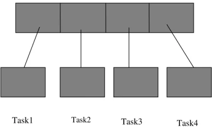
Data Partitioning is also often called data decomposition. In this type of partitioning, the data associated with a problem are decomposed into several relatively isolated parts. Each parallel task then works on a part of the partitioned data sets. As an example, in
Figure 2.1, the original data set is divided into four sub sets. Each of them is processed by a separate task.
The basic assumption in performing the partition is that the partitioned tasks ought to be equal or close to be equal size in term of computation effort required to complete the task, so that the workload on each machine can be balanced. The partitioned data sets are then processed on different processors. Therefore, distributing the data sets among the processors is another step following the partitioning. This is another important step in designing data decomposition based parallel schemes. It largely determines the efficiency of a parallel program.
Let T represent the data to be processed in a problem, and P be the set of processors. Data distribution can then be formally described by a function such as,
P T
DT : .
Task1 Task2 Task3 Task4
Figure 2.1. A data partitioning example, where the data is partitioned to 4 parts.
Therefore, DT1(p) gives the subset of the data T that will be processed by processor p. Assume the number of the partitioned data segments is N and the number of processors
is M, i.e., T ={d1,d2,d3,L,dN} and P={p1,p2,p3,L,pM}. Many different schemes can be employed to distribute these N data segments among the M processors. Two of the most fundamental ones are block distribution and round robin distribution, which are discussed in the following subsections.
a). Block distribution
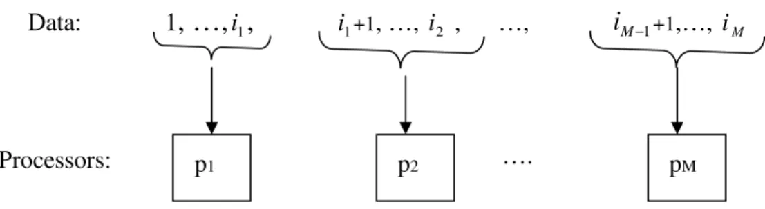
A block distribution refers to a scheme shown in Figure 2.2, i.e., sub-datasets 1, 2, …
1
i go to processor 1, i1+1, i1+2…, i are allocated to processor 2, etc.2
….
Mathematically, this scheme can be formulated as follows,
1 / ) 1 ( :d p= i M N + DT i .
Therefore, the partition to be processed by processor p will be
Data: 1
, …,
i1,
i1+1, …, i ,2 …, iM 1+1,…, iMp1 p2 pM
Processors:
}
{
p N M p N Mp
DT1( )= ( 1) / +1,..., /
It is obvious that each processor will have N/M data elements if N is dividable by M. This can be verified byp N/M
[
(p 1) N/M +1]
+1=N/M . However when N is not dividable by M, some processors will have floor(N/M) elements, others will have floor(N/M)+1 elements. Those having more data have an index p(l), such that). , mod( ,..., 2 , 1 , 1 ) , mod( ) 1 ( ) ( l N M M N M l l p = + =
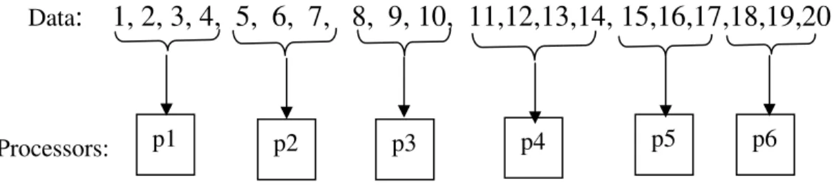
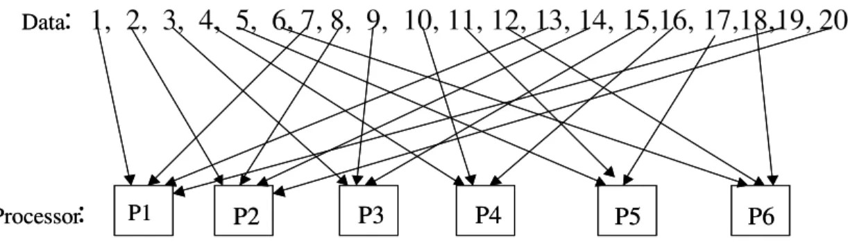
Using this block distribution scheme, the distribution of 20 (i.e. N=20) elements on 6 (i,e., M=6) processors is shown in Figure 2.3.
Here, mod(20,6)=2, 3 ) 6 , 20 mod( = M
. Therefore,p(1)=1, p(2)=4, i.e., the first and the 4thprocessor has 4 elements, each of the rest has 3 elements.
Data
:
1, 2, 3, 4, 5, 6, 7, 8, 9, 10, 11,12,13,14, 15,16,17,18,19,20
p2
p1 p3 p4 p5 p6
Processors:
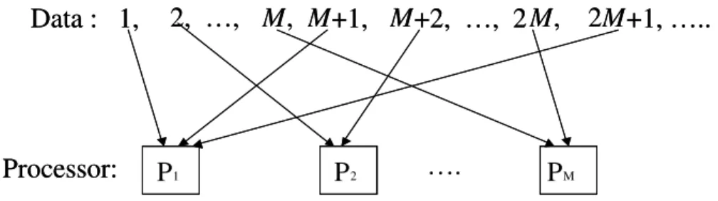
b). Round-robin distribution
Another convenient method to distribute N elements to M processors is the round-robin scheme as shown in Figure 2.4.
Mathematically, the formula describing the round-robin distribution scheme is given as follows: 1 ) , 1 mod( :d p = i M + DT i .
Therefore, the data sets for processor p will be
{
, ,2 ,...}
) ( 1 p M p M p p DT = + + .It is easy to show that each processor will have N/M elements if M is a factor of N. In the case that N is not dividable by M, each of the first mod(N,M) processors will have floor(N/M)+1 elements, the rest has floor(N/M) elements on each processor.
Data : 1, 2, …, M, M+1, M+2, …, 2 M, 2M+1, …..
Processor:
Data : 1, 2, …, M, M+1, M+2, …, 2 M, 2M+1, …..
Processor: P1 P2 …. PM
Using the round-robin distribution scheme, the 20 data elements are distributed among the 6 processors as shown in Figure 2.5, most of the processors have 3 elements, but p and1 p have 4 elements.2
Data distribution among processors is often relatively simpler than processing the data on each processor. In a parallel system, data on different processors may not be completely independent from others, certain communication may be required to complete a task. This problem will be addressed in detail from Chapter III through Chapter V.
2.2. Function partitioning
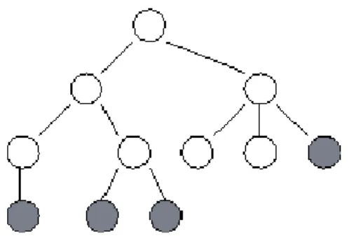
In this approach, the main focus is on the performed computation rather than on the data manipulated by the computation. The problem is decomposed based on the work that must be done. Each task then manipulates a portion of the work. A function partition decomposes not only the computation but also the performing code to reduce the complexity [3]. As an example, we explore a search tree that looks for nodes corresponding to a “solution”. The algorithm does not have any obvious data structure
Processor
:
Data:
1, 2, 3, 4, 5, 6, 7, 8, 9, 10, 11, 12, 13, 14, 15,16, 17,18,19, 20
P3 P1 P2 P4 P5 P6 Processor:
Data P3 P1 P2 P4 P5 P6that can be decomposed. Initially, a single task is created for the root of the tree. A task evaluates its node first, if that node is not a leaf, then it creates a new task for each search call (sub-tree). [17]
Figure 2.6. The structure of a search tree, in which each circle represents a node in the search tree and hence a call to the search procedure. A task is created for each node in the tree as it is expanded.
As shown in Figure 2.6, each circle represents a node in the search tree, and a call to the search procedure. A task is created for each node in the tree as it is explored. At any one time, some tasks are actively engaged in expanding the tree further; others that have reached solution nodes are terminating, or are waiting for their offsprings to report back with solutions.
In addition to above two commonly used partitioning schemes, sometime it is convenient to use such a scheme that employs both data and function decomposition. This is called mixed partitioning, which will be discussed in the following section.
2.3. Mixed partitioning of data and function
Combining the above two type of partitioning schemes is also common and natural. In many problems, a large amount of data is required to process. Data partitioning becomes a step that has to be implemented in order to complete the task. On the other hand, processing each partitioned data set may involve a significant amount of computation, which is very time consuming. An efficient algorithm requires the partitioning of the computation for each data set.
One example is the computation of wave propagation starting at different locations. Mathematically, the wave propagation is described by a wave equation given below,
) , , ( ) , , ( ) , , ( 2 2 2 2 2 2 y x t u t y x t u y y x t u x + = . (2.1)
where, u(t,x,y) is the wavefield at a spatial location (x,y) at time t .
To solve equation (2.1), we need to define two initial conditions for t , and four boundary conditions, two for x and two for y. The initial conditions define the initial state of the wave field; the boundary conditions, on the other hand, define constrains to the wave fields. For each initial state, the wave equation needs to be solved separately. The solution can be obtained using a 7-stencil method, which normally requires a large memory and computation.
Typical stencil methods include 5-stencil, 7-stencil, 9-stencil, etc. In general, a stencil is stylized matrix computation in which data at a group of neighboring elements are combined to calculate the one at a new location. They are typically combined in the form
of linear products. This type of computation is common in solving partial differential equations given in equation (2.1).
When the computation area is large, the large memory requirement becomes an issue. This problem can be overcome in a parallel program by partitioning the computation. On the other hand, in real applications, there are often a large number of such problems to be solved corresponding to a large number of different initial and boundary conditions. Then parallelization over the jobs is often required to get the job completed efficiently. The implementation of such a problem, which is often encountered in many applications, utilizes the partitioning of both the data and the functional computation.
In parallel computing, some programs require data communication or movement, while some others do not, where each processor will have sufficient information to complete its own task. Such parallel program is the easiest one to implement. Especially, by employing Python, the development of such a parallel code becomes trivial once a serial version of the code is available. In the following chapter, we will demonstrate the implementation of such a parallel code by solving a simple ray equation using Python to schedule and manage the serial executable that is built by the C compiler.
CHAPTER III
PARALLEL IMPLEMENTATION OF THE RAY EQUATION
Data communication is the most difficult part in designing a parallel program. Fortunately, in some applications, data communication can be avoided. One of these examples is to solve the ray equation given as follows,
) cos( ) ( ) ( ) sin( ) ( ) ( 1 1 k N cy k y k y k N cx k x k x n n n n + = + = + + , (3.1) where, ) sin( 2 1 ) ( 0 k N sx k x = + , cos( ) 2 1 ) ( 0 k N sy k y = + , (3.2)
and k = 0,1,2,3…K, n = 0,1,2,3,…N. cx, cy, sx, sy are all constants.
3.1. A serial C program
For any given cx, cy, sx, sy, the serial code to compute the ray points, xn+1(k) and )
(
1
k
yn+ is very simple. Figure 3.1 gives the pseudo-code that implements the ray equation in a serial mode. Assume this serial code produces an executable, ray.x. The job takes the starting location(sx,sy), the scalars cx,cyand the numbers K and N as input, and runs the executable to compute the values at all points defined by equation (3.1).
header file initialize define parameters
/*loop over the number of points to compute equation 3.2 */ when k<=K:
{
x[k]=sx+0.5*sin(PI/N*k); y[k]=sy+0.5*cos(PI/N*k); }
/*loop over the number of iteration to compute equation 3.1 */ when n<=N:
for (k=0;k<=K;k++) {
x[k]=x[k]+cx*sin(PI/N*k); y[k]=y[k]+cy*cos(PI/N*k);
write the results to a file }
Figure 3.1, A serial pseudo-code to compute the ray equation defined in equation 3.1 and 3.2.
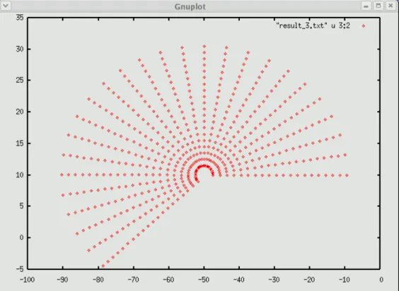
Figure (3.2) shows one of the solutions. In this example, cx=1, cy=2, sx=10, sy= 50 and K =25, N =20.
Figure 3.2. One example of the ray equation generated by a serial C code, where, cx =1, cy = 2, sx =10, sy = -50, and K = 25, N = 20.
Even though the computation of one job at one location is rather small, the computation can be accumulated dramatically if a large number of jobs are required to compute the rays which corresponds to different input parameters; i.e., different starting points. Apparently, the task can be simply set up by paralleling over the jobs using any language, since no communication is required between jobs for different points. Here we use it as an example to demonstrate the applicability of combining Python with the serial executable, ray.x. In this example, Python is used to design a script to set up and manage the jobs over different processors.
3.2. A Parallel Python Script
In the above example, as no communication is needed among different jobs that compute rays for different starting locations, parallel computation of different jobs can be simply implemented by executing the serial job on each processor. For that purpose, the serial executable, ray.x, and the parameters required by each job need to be copied to each processor so that each job can execute locally on each processor.
Obviously, the structure of a parallel code heavily depends on the hardware configuration. As an example, we implement it on a computer system that has distributed memory. In fact, they are independent machines connected together through a network. There are no shared resources among the different machines at all.
Since different processors do not share any resources, we first distribute the executable to those processors so that the serial code can run independently on different processors. A pseudo Python script that distributes the executable, ray.x, is shown in
Figure 3.3. It invokes the “rcp” command to copy it remotely to each processor. The job is started up on each processor by a system command call:
commands.getstatusoutput(cmd).
for machine in machinelist:
cmd="rcp /home/folder/ray.x machine:directory " stat,out=commands.getstatusoutput(cmd)
Figure 3.3. A pseudo Python script to distribute the executable to remote machines
Next, we need a similar python script to distribute the required parameters to those processors and start the executable on each machine. Here we assign the jobs among the different computers in a round-robin fashion. The execution of the jobs is initiated by the system call, commands.getstatusoutput(cmd). The pseudo Python script that completes this task is shown in Figure 3.4.
get the parameter file get the machine name list
separate the parameters distribute the job
cmd0="/home/directory/ray.x + parameters+ job_id for machine in machinelist:
cmd="rsh "+machine + cmd0 /* submit the job to a remote machine */ stat,out=commands.getstatusoutput(cmd)
Figure 3.4. A pseudo Python script to execute the job on different processors.
Each job will produce an output file with a unique name consisting of a base name “result_” and a unique number (this is defined in the C executable). However, those output files may locate on the local disks of different computers, which need to be collected to a central location. This is also implemented through a Python script by executing the “rcp” command as shown in Figure 3.5.
for machine in machinelist:
cmd="rcp machine:directory/result*.txt /home/directory/central directory " stat,out=commands.getstatusoutput(cmd)
Figure 3.5. A pseudo Python script to collect the results to a machine.
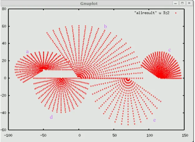
As an example, Figure 3.6 shows the results of the ray equation for 5 different jobs corresponding to 5 different starting points. They are computed in parallel on 3 different machines.
Figure 3.6. Ray tracing results of 5 different jobs computed on 3 different machines using a parallel Python script. Job a, d are executed by machine 1. Job b, e are executed by machine 2. Job c is executed by machine 3. They differ each other by different combination of sx, sy, cx and cy.
a
b
c
d
In this simple example, we demonstrate that when no communication is required, a parallel software can be implemented simply from a serial code using Python script, which largely simplifies the development effort needed using a compiled language.
The above example is very simple, but quite illustrative, it demonstrates the robustness of combining Python with a compiled language C to design a parallel program that virtually has no data communication during execution. However, most parallel applications are not that simple. In most cases, they do require different processors to share data and communicate with each other during the execution. For example, the wave propagation problem in equation (2.1) requires a processor to know the information calculated by its neighboring processors if it is solved in parallel. This problem is investigated in detail in the following chapters.
CHAPTER IV
PARALLEL IMPLEMENTATION OF THE 1-D PARTIAL DIFFERENTIAL WAVE EQUATION USING PYTHON AND C
Partial differential equations (PDE) describe a wide range of phenomena in science and engineering [7]. Efficiently solving these PDEs has significant importance for both scientific research and engineering applications. Typically, solving a PDE involves a large amount of data and computation. A parallel program that solves this problem is usually developed in a compiled language such as C/C++ by using message passing interface (MPI). However, similar to the demonstration in the last Chapter, Python offers a quite convenient environment to solve the PDE.
In this chapter, we use Python to implement a parallel program on multiple processors to solve the PDE. Since the one-dimensional problem is much simpler and still illustrative, we focus on discussing the one-dimensional partial differential equations in this chapter.
4.1. The One-dimensional Partial Differential Equation
The basic one dimensional partial differential equation (PDE) is a second order wave equation as follows,
) , ( ) , ( 2 2 2 2 2 x t u x C x t u t = . (4.1)
Where t stands for time, x is the spatial variable and C is the wave propagation velocity. Solving this equation requires two initial conditions for variable t, as given below,
) ( | ) , (t x 0 f x u t= = , (4.2) ) ( | ) , (t x 0 g x u t t= = , (4.3)
and two boundary conditions for x, such as, ) ( | ) , ( min s t x t u x=x = , ) ( | ) , ( max r t x t u x=x = . (4.4)
Equations (4.1)-(4.4) can be used to model waves on a string, waves in a flute, and in a rod, etc. Here, f(x) and g(x) define the initial state. s(t) and r(t) define the constrains at both ends.
4.2. Numerical method
In order to numerically solve the PDE in equations (4.1) - (4.4), we need to use a finite difference scheme to approximate the 2ndorder derivatives with respective to t and x. A finite difference approximation to the derivatives in equation 4.1 can be written as,
2 2 2 2 2 ) , 1 ( ) , ( 2 ) , 1 ( ) , ( ) , ( t j i u j i u j i u x j t i u t x t u t + + = = , (4.5)
and 2 2 2 2 2 2 2 2 ) 1 , ( ) , ( 2 ) 1 , ( ) , ( ) , ( x j i u j i u j i u C x j t i u x C x t u x C + + = = . (4.6) Therefore, 2 2 2 ) 1 , ( ) , ( 2 ) 1 , ( ) , 1 ( ) , ( 2 ) , 1 ( x j i u j i u j i u C t j i u j i u j i u + + = + + , (4.7) or,
[
]
) , 1 ( ) 1 , ( ) , ( ) 1 ( 2 ) 1 , ( ) , 1 ( ) , ( 2 ) 1 , ( ) , ( 2 ) 1 , ( ) , 1 ( 2 2 2 j i u j i Au j i u A j i Au j i u j i u j i u j i u j i u x t C j i u + + + = + + + = + . (4.8) Where 2 2 2 x t CA= , i is the index for t , and j is the index for x.
As shown in Figure 4.1, the finite difference equation (4.8) defines the relationship among the 5 points, which is typically called a 5-stencil. From the given equation (4.2), we know the values at i=0. Together with equation (4.3), we can compute all the values at i = 1. Then using equation (4.8), we can compute all the values at i=1. Similarly, from the known values at i=0 and 1, we can use equation (4.8) again to compute all the values at i=2, and so on. Such process can be represented in a matrix form concisely as follows, 1 1 + = i + i i U BU U . (4.9) Where, T x i i N u i u i u i u
U =[ (1, ), (2, ), (3, ),..., ( , )] is a vector with N entries,x and
= ) 1 ( 2 0 0 0 0 ) 1 ( 2 0 0 0 0 ) 1 ( 2 0 0 0 0 ), 1 ( 2 A A A A A A A A A A B L L L M M O M M M L L L L L L (4.10)
is a NX ×NX tri-diagonal matrix, which has at most 3 non-zero elements in each row.
Figure 4.1. A 5-stencil diagram used in solving equation (4.8).
4.3. Numerical solution
A parallel program can be developed using Python to solve the one dimensional PDE approximated by the iterative matrix equation (4.9). For simplicity, we choose
) sin( )
(x x
f = , g(x)=0, C=1 and s(t)=0, r(t)=0.
The range for x is (0,10 ). This problem has an exact solution, which is, i-1
i+1
i
Ct x Ct x Ct x x t
u sin( ) sin( ) sin cos
2 1 ) ,
( = + + = .
For each constant t, u( xt, )is a sine function scaled bycosCt. We use 91 discrete grid points in the range (0,10 ) for x; therefore, the sample interval in the x-direction is x=10 /(91 1). The sample rate along the t-direction is chosen as t = x. Figures 4.2 – 4.4, show this exact function at 3 different times t =1 t, 3 t and 6 t, respectively.
Figure 4.2. An exact solution of the PDE in equation 4.1 at t =1 t.
Figure 4.4. An exact solution of the PDE in equation 4.1 at t =6 t.
In designing this parallel program, we partition the computation grids among the multiple processors. For this 1-D problem, this task is rather simple. Nevertheless, it is still illustrative to understand the partitioning scheme and the power of Python in parallel numerical computation. As we can see in the iterative matrix equation (4.9) and the 5-stencil scheme in Figure 4.1, the values at t =(i+1) tare fully defined by the values at
t i
t = and t =(i 1) t. Therefore, a natural way to partition the problem is along the x-direction, as shown in Figure 4.5.
Assume the total number of grid points Nx is dividable by the number of processorsNp. We use the block distribution scheme discussed in chapter 2 to partition them; i.e., define Nx =Nx/Np. So, grid nodes 1, 2, …Nx will be assigned to processor 1, grid nodes (Nx +1), (Nx+2), … 2Nx will be assigned to processor 2, …
x
p N
N 1)
( +1, (Np 1) Nx +2, …Np Nx will be assigned to processor Np. Suppose we are going to implement the computation on 3 processors and iterate 10 steps. i.e., 1 j 90,1 i 10. Each processor has 30 nodes in the x-direction. Processor P ’sk
Figure 4.5. Partitioning scheme in solving the 1-D PDE. a): All the interior nodes for each processor can be computed easily from equation (4.8), since all the required information is available in the same processor. b): The data at the two ends of each processor are shared by neighboring processors, which should be communicated between the nodes. These shared grid points form “ghost” layers.
x
t
…
…
…
…
…
…
…
…
…
…
…
…
…
…
…
…
K P 1 K P PK+1a)
b)
ghost layers ghost layers
i i - 1 i + 1 i + 1 i + 1 i j + 1 j - 1 j j - 1 j j + 1
nodes are from 30 (k-1)+1 to 30 k. All the interior nodes for each processor can be computed easily from equation (4.8), since all the required information is available in the same processor (see Figure 4.5 a). However problems arise for the grid nodes at both ends as we can see in Figure 4.5, where, to compute the first node of processor P on thek left, one needs the information of the last node on the right of processor PK 1; Similarly, to compute the last node on the right of processor P , one requires the data at the firstK node on the left of processor PK+1. Therefore, the data at the two ends of each processor are shared by neighboring processors. These shared grid points form “ghost” layers (see Figure 4.5 b). Communications are required between neighbor processors in the ghost layers. Python makes this communication quite easy by using pypar.send and pypar.receive. Those constructs are equivalent to MPI_Send and MPI_Recv in C. The
pseudo code that solves the one-dimensional partial differential equation is shown as follows.
Define the number of nodes n
define the number of processors pronum
partition the work to the processors, each processor contains x_sml=n/pronum nodes Allocate memory, each processor should hold x_sml+2 nodes
t=0
Set Initial condition: u[xi]= sin(xi), i=0,…,x_sml+1 Set the boundary condition
Define the value of one time before and one time after the u as um & up while t<t_stop
exchange the ghost layer value, communication is needed here update all inner point:
save the result to a disk file plot result if requested
initialize for the next step: um=u, u=up update the time step: t=t+dt
Figure 4.6. A pseudo code for the one-dimensional partial differential equation. We develop two separate codes, one using Python and another using C, to do the
1D space direction, the code is quite simple, the ghost layer communication can be implemented using the following pseudo-code,
If it has right neighbor:
copy u[:,x_sml] to right neighbor’s first column u[:,0]
If it has left neighbor:
copy u[:,1] to left neighbor’s last column u[:, x_sml+1]
Figure 4.7. A pseudo-code for updating the ghost layers
4.4 Numerical results
To verify the program, we show the computed wave field u( xt, )at t = 1 t, 3 t, 6 t, respectively in Figure 4.8 – 4.10. Comparing with the exact theoretical results shown in Figure 4.2 – 4.4, we see that the code produced the expected results.
Figure 4.9. Numerical result of the 1D PDE at t =3 t from the python code.
Figure 4.10. Numerical result of the 1D PDE at t =6 t from the python code.
To Compare with the Python code, we also show the results of the program developed in C at t = t, 3 t, 6 t, ( t=0.05) respectively in Figure 4.11 – 4.13. We can see that the results of both the python and the C programs are the same.
Figure 4.11. Numerical result of the 1D PDE at t = t from the C code.
Figure 4.12. Numerical result of the 1D PDE at t =3 t from the C code.
CHAPTER V
PARALLEL IMPLEMENTATION OF THE 2-D PARTIAL DIFFERENTIAL WAVE EQUATION USING PYTHON AND C
In this chapter, we investigate the applicability of Python for designing parallel programs to solve a more complicated 7-stencil problem, which solves the two-dimensional partial differential equation. This equation describes the propagation of water waves, seismic waves, etc. As expected, this problem is much more complicated compared to the 5-stencil problem discussed in the previous chapter.
5.1. Two-dimensional partial differential wave equation
The two-dimensional partial differential wave equation is formulated as, ) , , ( ) ( ) , , ( 2 2 2 2 2 2 2 y x t u y x C y x t u t = + . (5.1)
Where, t stands for time, x,y are the two spatial variables. Similar to the 1-D case, Solving equation (5.1) requires two initial conditions at t=0, such as,
) , ( | ) , , (t x y 0 f x y u t= = , ) , ( | ) , , (t x y 0 g x y u t t= = . (5.2)
) , ( | ) , , ( 1 min a t y y x t u x=x = , ) , ( | ) , , (t x y max a2 t y u x=x = . (5.3) and ) , ( | ) , , (t x y min b1 t x u y=y = , ) , ( | ) , , ( 2 max b t x y x t u y=y = . (5.4)
Where, f(x,y), g(x,y) define the initial state of the wave described by equation (5.1), 2 , 1 ), , ( ), , (t y b t x i=
ai i define the boundary constrains to the field.
5.2. Numerical Method
Like the 1-D problem discussed in chapter IV, solving equation (5.1) to (5.4) requires finite difference approximations to all the partial derivatives. In addition to the difference operators defined in equations (4.5) and (4.6) that approximate the derivatives to t and
x , we also need a similar operator for the derivative with respect to y, i.e.,
2 2 2 2 2 ) , , 1 ( ) , , ( 2 ) , , 1 ( ) , , ( ) , , ( t k j i u k j i u k j i u y k x j t i u t y x t u t + + = = , (5.5) 2 2 2 2 2 2 2 2 ) , 1 , ( ) , , ( 2 ) , 1 , ( ) , , ( ) , , ( x k j i u k j i u k j i u C y k x j t i u x C y x t u x C + + = = , (5.6) and
2 2 2 2 2 2 2 2 ) 1 , , ( ) , , ( 2 ) 1 , , ( ) , , ( ) , , ( y k j i u k j i u k j i u C y k x j t i u y C y x t u y C + + = = . (5.7)
After substituting (5.5), (5.6) and (5.7) to equation (5.1), we get,
) , , 1 ( ) 1 , , ( ) 1 , , ( ) , 1 , ( ) , , ( ) 1 ( 2 ) , 1 , ( ) , , 1 ( k j i u k j i Bu k j i Bu k j i Au k j i u B A k j i Au k j i u + + + + + + = + (5.8) where, 2 2 2 2 2 2 , y t C B x t C A = = .
Equation (5.8) defines the relationship among 7 neighboring grid points as shown in Figure 5.1, which is a typical example of a 7-stencil problem.
Figure 5.1. A 7-stencil diagram used in solving the 2D partial differential equation. i-1 i+1 i j-1 j j+1 k-1 k k+1 t y x
5.3. Data partitioning
Like the 1-D case, in designing a parallel program to solve the two-dimensional PDE, a natural way to partition the data is to partition it on the x-y plane. In this plane, the grid points form a 5-stencil problem. Generally, this 2D plane can be partitioned in one of the three different ways shown in Figure 5.2.
a)
b)
c)
Figure 5.2. Three partitioning schemes for a 2D plane to solve the 2D PDE.
Partitioning methods b) and c) are similar to the scheme used in the 1-D problem (Figure 4.5). Thus, to avoid the redundancy, in this chapter, we use method a) to demonstrate the implementation of a parallel program on multiple processors using Python. As an example, we define the sampling dimensions asNx×Ny =12×9=108, which are divided among × =3×3=9
y
x P
P N
each processor has 4 nodes in the x-direction, and 3 nodes in the y-direction. More specifically, the partition parameters are given as follows,
y
x P
P N
N
P= × = 9 is the total number of processors,
x P
N = 3 is the number of partitions in x-direction,
2
Figure 5.3. One partitioning scheme for a 2D plane used in solving a 2D PDE. ipx, ipy represent the processor index along x and y direction, respectively.
y P
N = 3 is the number of partitions in y-direction,
x
N = 12 is the number of nodes in x-direction,
y
N = 9 is the number of nodes in y-direction, sml
x
N _ = N /x x P
N = 12 / 3 = 4 is the number of nodes in each processor in x-direction,
y
x
0 1 2 3 4 5 6 7 8 9 10 11 0 1 5 2 3 6 4 7 P3 P1 P4 P2 P5ipy
ipx
0
1
2
0
1
P0 8 P6 P7 P8sml y
N _ = Ny/ N = 9 / 3 = 3 is the number of nodes in each processor in y-direction.Py If we use 2-dimensional matrices to represent the nodes in each processor, we have,
= 3 , 2 2 , 2 1 , 2 0 , 2 3 , 1 2 , 1 1 , 1 0 , 1 3 , 0 2 , 0 1 , 0 0 , 0 0 a a a a a a a a a a a a MP , = 7 , 2 6 , 2 5 , 2 4 , 2 7 , 1 6 , 1 5 , 1 4 , 1 7 , 0 6 , 0 5 , 0 4 , 0 1 a a a a a a a a a a a a MP , = 11 , 2 10 , 2 9 , 2 8 , 2 11 , 1 10 , 1 9 , 1 8 , 1 11 , 0 10 , 0 9 , 0 8 , 0 2 a a a a a a a a a a a a MP , = 3 , 5 2 , 5 1 , 5 0 , 5 3 , 4 2 , 4 1 , 4 0 , 4 3 , 3 2 , 3 1 , 3 0 , 3 3 a a a a a a a a a a a a MP , = 7 , 5 6 , 5 5 , 5 4 , 5 7 , 4 6 , 4 5 , 4 4 , 4 7 , 3 6 , 3 5 , 3 4 , 3 4 a a a a a a a a a a a a MP , = 11 , 5 10 , 5 9 , 5 8 , 5 11 , 4 10 , 4 9 , 4 8 , 4 11 , 3 10 , 3 9 , 3 8 , 3 5 a a a a a a a a a a a a MP , = 3 , 8 2 , 8 1 , 8 0 , 8 3 , 7 2 , 7 1 , 7 0 , 7 3 , 6 2 , 6 1 , 6 0 , 6 6 a a a a a a a a a a a a MP , = 7 , 8 6 , 8 5 , 8 4 , 8 7 , 7 6 , 7 5 , 7 4 , 7 7 , 6 6 , 6 5 , 6 4 , 6 7 a a a a a a a a a a a a MP , = 11 , 8 10 , 8 9 , 8 8 , 8 11 , 7 10 , 7 9 , 7 8 , 7 11 , 6 10 , 6 9 , 6 8 , 6 8 a a a a a a a a a a a a MP .
Suppose we use ipx, ipy to represent the processor index along x and y direction respectively. Then the index of each processor can be represented asP ipy N ipx
x P
k = × + .
The index of the nodes belonging to one processor will range from Nx_sml×(ipx 1)+1 to Nx_sml×ipx along the x direction and from Ny_sml×(ipy 1)+1 to Ny_sml×ipy along the y direction.
5.4. Data communication
Similar to the one-dimensional problem in Chapter IV, communication along the boundary of each processor is required to solve the 7-stencil problem. However, the 2D case is much more complicated. As we need to combine the values on a 5-stencils at
t i
t = and one value at t =(i 1) t to compute one value at a new location at
t i
t =( +1) (equation 5.8). Communication is required on the nodes of the 5-stencil plane (Figure 5.4) at t=i t. Those operations are carried out on the entire two-dimensional plane. The partition in Figure 5.2 a) requires communication along both x and y directions. As in the one-dimensional case, the communicated nodes form ghost layers. However, in this case the ghost layers run along both x and y directions as shown in Figure 5.4 by the dotted-boxes. Because of the “data sharing” on the internal boundaries between neighboring processors for the 5-stencil operation, the actual data each processor needs must include those within the ghost layers.
5.5. Numerical Results
In this section, we complete a numerical experiment of a parallel code developed using Python to solve the 2D PDE. In this example, we use 8 processors, 4 in x and 2 in y
direction. We choose = 2 ) 2 / ( 2 ) 2 / ( 2 2 ) , ( Ly y Lx x e y x f , g(x,y)=0, and a1(t,y)=0, 0 ) , ( 2 t y =
a , b1(t,x)=0, b2(t,x)=0. The ranges for both x and y are both(0,10). We discretize the range to 40 grid points in each direction. Therefore, the sample interval
25 . 0 ) 1 40 /( 10 = = y
x . For numerical stability, we choose the sample rate along t-direction as t = 0.2, c = 1.
Figure 5.4. A two dimensional grid map partitioned for solving the 2D partial differential equation in parallel. The dotted boxes include the communicating nodes between 2 adjacent processors, which form ghost layers.
The pseudo-code for the 2D partial differential equation is given as follows, Define the number of points nx,ny
define the number of processors Np
define the partition in both x and y directions, Npx,Npy distribute the work to the processors,
each processor contains x_sml = nx/Npx nodes in x direction and y_sml = ny/Npy nodes in y direction
Allocate enough memory, each processor can hold (x_sml+2)*(y_sml+2) nodes Define function exchmsg(), which exchange data in ghost layers
Set Initial condition: u[x ,i yj]=
2 ) 2 / ( 2 ) 2 / (xi Lx 2 yj Ly 2 e , i=0,…,x_sml+1, j=0,…,y_sml+1
Set the boundary condition
compute the value of one time step before t=0 using the initial conditions while t<t_stop
call exchmsg() to exchange the ghost layer update all inner point using equation 5.8
for i=1,…,x_sml, j=1,…,y_sml
concatenate result from each processor send its result to the first one ghost layer
save the result to a disk file update the time step by t=t+dt plot result
_____________________________________________________________________
Figure 5.5. A pseudo code to solve the 2D PDE.
Although the pseudo-code is easy and can be implemented in both C and Python, there are several key differences when it is implemented using the two languages. Some of them are listed below,
1. 2D array memory allocation in Python is much easier than in C. Allocation in Python: u=zeros((nx_sml+2,ny_sml+2),Float) um=zeros((nx_sml+2,ny_sml+2),Float) up=zeros((nx_sml+2,ny_sml+2),Float) Allocation in C: u=(double**)malloc((nx_loc+2)*sizeof(double*)); up=(double**)malloc((nx_loc+2)*sizeof(double*)); um=(double**)malloc((nx_loc+2)*sizeof(double*)); for(i=0;i<nx_loc+2;i++){ u[i]=(double*)malloc((ny_loc+2)*sizeof(double)); up[i]=(double*)malloc((ny_loc+2)*sizeof(double)); um[i]=(double*)malloc((ny_loc+2)*sizeof(double)); }
Therefore, Python directly allocates space for 2D arrays, while C has to complete this in 2 steps, where, a 2D array is defined as an array of pointers. In the first step, memory is allocated to the array of pointer, then memory is allocated to each of the pointers.
2. Message exchanging in Python is easier than in C as we mentioned in Chapter I. Python only needs to know what is the source for receiving data and what is the destination for sending data. But, MPI_Send and MPI_Recv both require to specify the size, data type, communicator in addition to the source and destination.
#---# exchange y - boundary #---source destination if ipy!=nyproc-1: pypar.send(u_loc[:,ny_sml],destination) if ipy==0: u_loc[:,0]=0 else: u_loc[:,0]=pypar.receive(source)
Part of a Python code to exchange data in the y direction.
/* exchange y - boundary */ if (ipy!=nyproc-1) {
/* send to upper neighbor */
MPI_Send (syrbd,nx_loc+2,MPI_DOUBLE,destination,Tag,MPI_COMM_WORLD); }
if (ipy==0){
for (i=0; i<=nx_loc+1; i++) rylbd[i]=0;
}
/* receive from upper neighbor */ else {
MPI_Recv(rylbd,nx_loc+2,MPI_DOUBLE,source,Tag,MPI_COMM_WORLD,&status); }
Part of a C code to exchange data in y direction.
3. The concatenation function defined in Python makes the handling of output very convenient. Python can call function concatenate to glue the results together.
#---# concatinate the result #---source=myid-1 destination=(myid+1)%numproc if ipx==0: pypar.send(a, destination) elif ipx==nxproc-1: result = pypar.receive(source) result=concatenate((result,a)) source = myid-nxproc destination = (myid+nxproc)%numproc if ipy==0: pypar.send(result,myid+nxproc) elif ipy==nyproc-1: result0 = pypar.receive(source) result1=concatenate((result0,result),1) else: result0 = pypar.receive(source) result1=concatenate((result0,result),1) pypar.send(result1, destination) else result= pypar.receive(source)
result= concatenate((result,a)) pypar.send(result,destination)
___________________________________________________________________
Python code to concatenate the result from all processors.
4. Implementing a visualization software in C is time consuming, but it is very simple in Python. In fact, this is one of the many advantages that makes Python popular. The outputs for the Python and the C programs are discussed in the next section.
5.6. Visualization
Scientific applications often involve graphic visualization of the results. Professional-looking graphs need fine tunings of tick-marks on axis, colors and line-styles, etc [7]. Developing a plotting program that gives a professional look to graphs is a challenging and very time-consuming task for most programming languages. Gnuplot is a popular and easy to use open-source plotting program. It is a portable command-line driven interactive data and function plotting utility for UNIX and many other platforms. It supports many different types of plots in both 2D and 3D. It can draw lines, points, boxes, contours, vector fields, surfaces etc. It also supports various specialized plot types [16].
By interfacing Python to Gnuplot, we can easily design a visualization software for data files or mathematical functions. In the 2D PDE Python program, we directly import Gnuplot package to the python code, and display the results, which are actually 3D data volumes. Some of the results are shown in Figure 5.6.
For comparison, we also developed a separate Python script, which is an interface for Gnuplot to plot the result of the C program designed using MPI. In this script, it reads the results of the C program from a disk file; then, it initiates the Gnuplot to plot the result. Some of the C program results are shown in Figure 5.7. They are exactly the same as the corresponding results shown in Figure 5.6. Therefore, both the Python and C codes produce the same results, but the implementation using Python is much simpler.
a b
c d
e f
Figure 5.6. Numerical results of the 2D PDE implemented using Python, where a) to f) are the solution at t = 0.0, 0.6s, 1.2s, 1.8s, 3.2s, 4.6s, respectively.
a b
c d
e f
Figure 5.7. Numerical results of the 2D PDE implemented in C using MPI, where (a) to (f) are the solutions at t = 0.0, 0.6s, 1.2s, 1.8s, 3.2s, 4.6s, respectively.
CHAPTER VI
EXTENDING PYTHON WITH C FOR SCIENTIFIC COMPUTATION
In Chapter IV and Chapter V, we have implemented the parallel software for the 1D and 2D partial differential wave equations using Python and C separately. However, C is optimized for speed of execution, but a C program is complicated to develop, especially in parallel implementation. Python is optimized for speed of development, but the execution of a numerical computation software developed in Python is much slower.
In this chapter, we are going to optimize the program by combing Python and C together. Most languages offer the possibility to call functions written in other languages. In Python, this is a particularly simple and smooth process, since Python was initially designed for integration with C and C++. Integration of Python with C or C++ codes requires a communication layer, called a wrapper. The integration includes: 1) migration of slow code; 2) accessing to the existing numerical codes. In both cases, we want to benefit from using Python for non-numerical tasks. In most scientific computing programs, only a small part of the total code is CPU time intensive. Writing a scientific computing application in Python and moving CPU-time critical parts to a compiled language like C can take advantages of both languages [7]. As an example, we will repeat the implementation of the software to solve the 2D PDE.
Calling a function written in a compiled language from Python is not a trivial task. In Python, each variable is an object, it does not have a specific type. However, in a compiled language, each variable can only hold one type, like int, float etc in the C language. It needs a wrapper as the interface between a language with strong typing like C and dynamically typed language like Python. There are rules available for sending variables between Python and C [7]. A wrapper function, written in C, typically takes two arguments, self and args, where self only deals with instance methods, while args holds a tuple of the arguments sent from Python. Writing wrapper functions requires knowledge of how Python objects are manipulated in a C code. Fortunately, when combining Python with C, there is no need to concern about different storage schemes. In the next section, we are going to discuss the issues in writing the wrapper in C.
6.1. Implementing a C wrapper
It is quite easy to add new built-in modules to Python when one knows how to program in C. Such extending modules can do two things that can’t be done directly in Python: they can implement new built-in object types, and they can call C library functions and initialize system calls [4]. The structure of an extending file usually contains the following parts:
• The functions that make up the module
• A method table that lists the functions to be called from Python • The module’s initialization function
In our extended program, we convert the computational part to C from Python in a file named cloops.c, where, we create a function stencil_pde, which is the accessing point from Python, and it gives the complete control of all details of the Python-C interface.
Head files are needed to access the Python and NumPy C API in our extension module. Since Python can contain some pre-processing definitions that may affect the standard headers on some system, it is usually required to include the Python.h in the first line of the C file cloops.c. To make Numpy arrays available to an extension module in C, it must include the header file arrayobject.h in the C function.
The function stencil_pde provides straightforward translation from the argument list in Python to the arguments passed to the C function. It first uses PyArg_ParseTuple function to parse arguments and extract the individual variables, then proceeds computations and returns the results to the Python caller.
Method table lists all the C functions to be called from Python. Names in the table become muddle attribute names that Python code uses to call the C function. Pointers in this table are used by interpreter to dispatch C function calls.
Initialization function is provided by C function cloops.c. Once initialized, calls from Python are routed directly to the C function through the method table’s function pointer.
The pseudo-code of cloops.c is showed as follows, where stencil_pde(…) is the function which can be called from Python directly.
Header file Method function:
using PyArg_ParseTuple(args,"O!O!O!dd:stencil_pde", &PyArray_Type,&u_array,
&PyArray_Type,&um_array, &PyArray_Type,&up_array, &Cx2,&Cy2))
get array lenth nx and ny
let direct access to the data as 1D array u=(double*)u_array->data;
um=(double*)um_array->data; up=(double*)up_array->data; define offset
calculate the result return to Python caller }
The method table
- it lists the functions that should be callable from Python: static PyMethodDef MethodTable[] = {
{"stencil_pde", stencil_pde, METH_VARARGS },
{NULL, NULL} /* required ending of the method table */ };
Initialization function void initcloops(void) {
PyObject *m = Py_InitModule("cloops", MethodTable);
import_array() /*which is required for NumPy initialization */ }
Figure 6.1. A pseudo code for the computation intensive core extended in C.
6.2. Compiling and linking
Compiling and linking are the two important steps to do before we can use the extension. Here, we use a sh file to create a .so file cloops.so that Python can automatically find. The sh file is given in the following:
#!/bin/sh -x
# build the C extensions modules cloops # from cloops.c
root=`python -c 'import sys; print sys.prefix'` ver=`python -c 'import sys; print sys.version[:3]'` module=cloops
gcc -O3 -g -I$root/include/python$ver \ -I$/home/directory \
-c $module.c -o $module.o gcc -shared -o $module.so $module.o
# test the module:
python -c "import $module; print dir($module)" if [ $? -ne 0 ]; then
echo "Unsuccessful build of $module" exit
fi
6.3. Calling a C function from Python
To use the C function stencil_pde inside a Python file, only two lines of code given below are needed comparing to the original Python code in chapter V:
from cloops import stencil_pde stencil_pde(u,um,up, …)
The pseudo python code that extends the C function is shown below. Import useful functions
...
from cloops import stencil_pde ...
Define the number of nodes nx,ny
define the number of processors Np, and in x , y directions Npx,Npy Divide the work to the processors,
each processor contains x_sml=nx/Npx nodes in x direction each processor contains y_sml=ny/Npy nodes in y direction Allocate enough memory, each processor can hold (x_sml+2)*(y_sml+2) nodes Define function exchmsg(), which changes data in ghost layer
t=0
Set Initial condition: u[x ,i yj]=
2 ) 2 / ( 2 ) 2 / (x Lx 2 y Ly 2 e , i=0,…,x_sml+1, j=0,…,y_sml+1
Set the boundary condition
Compute the value of one time step before t=0 as um while t<t_stop
call exchmsg()
update all inner point:
using equation (5.8) for i=1,…,x_sml, j=1,…,y_sml
call stencil_pde(u_loc,um_loc,up_loc,Cx2,Cy2) to calculate the result store the result to file
plot result
update the time step t=t+dt
Figure 6.3. The pseudo Python code with C extension to solve the 2D PDE. We can see that in this code, only the two blue lines are different with Figure 5.5.
6.4. Run time comparison
![Figure 1.1. The long-term trends for the first 10 programming languages [15].](https://thumb-us.123doks.com/thumbv2/123dok_us/504173.2559485/10.918.169.803.227.674/figure-long-term-trends-programming-languages.webp)