COBAYN: Compiler autotuning framework using Bayesian networks

(1)

Amir Hossein Ashouri, Giovanni Mariani, Gianluca Palermo, Eunjung Park,

John Cavazos, Cristina Silvano

COBAYN: Compiler Autotuning Framework using Bayesian Networks

ACM Transactions on Architecture and Code Optimization

The published version is available online at: http://dx.doi.org/10.1145/2928270

c

2018 ACM. Personal use of this material is permitted. Permission from the editor must be

obtained for all other uses, in any current or future media, including reprinting/republishing this material for advertising or promotional purposes, creating new collective works, for resale or redistribution to servers or lists, or reuse of any copyrighted component of this work in other works.

(2)

AMIR HOSSEIN ASHOURI, Politecnico di Milano, ITALY

GIOVANNI MARIANI, IBM, The NETHERLANDS

GIANLUCA PALERMO, Politecnico di Milano, ITALY

EUNJUNG PARK, Los Alamos National Laboratory, USA

JOHN CAVAZOS, University of Delaware, USA

CRISTINA SILVANO, Politecnico di Milano, ITALY

The variety of today’s architectures forces programmers to spend efforts for porting and tuning application codes across different platforms. Compilers themselves need additional tuning which has considerable complexity as the standard optimization levels, usually designed for the average case and the specific target architecture, quite often fail to bring the best results.

This paper proposesCOBAYN: COmpiler autotuning framework using BAYesian Networks, an approach for a

compiler autotuning methodology using machine learning to speed up application performance and to reduce the cost of the compiler optimization phases. The proposed framework is based on the application characterization done dynamically by using independent micro-architecture features and Bayesian networks. The paper also presents an evaluation based on using static analysis and hybrid feature collection approaches. In addition, the paper compares Bayesian networks with respect to several state-of-the-art machine-learning models.

Experiments were carried out on an ARM embedded platform and GCC compiler by considering two benchmark suites with 39 applications. The set of compiler configurations selected by the model (less than 7% of the search space),

demonstrated an application performance speedup of up to 4.6×on Polybench (1.85×on average) and 3.1×on cBench

(1.54×on average) with respect to standard optimization levels. Moreover, the comparison of the proposed technique

with (i) random iterative compilation, (ii) machine learning-based iterative compilation and (iii) non-iterative

pre-dictive modeling techniques, shows on average, 1.2×, 1.37×and 1.48×speedup, respectively. Finally, the proposed

method demonstrates 4×and 3×speedup, respectively on cBench and Polybench, in terms of exploration efficiency

given the same quality of the solutions generated by the random iterative compilation model.

Categories and Subject Descriptors: D.3.4 [Programming Languages]: Processors—Compilers

CCS Concepts: rSoftware and its engineering → Compilers; rComputing methodologies→ Supervised

learning;rMathematics of computing→Bayesian networks;

General Terms: Autotuning, Compilers, Machine Learning, Performance Evaluation

Additional Key Words and Phrases: Bayesian Networks, Statistical Inference, Design Space Exploration ACM Reference Format:

Amir Hossein Ashouri, Giovanni Mariani, Gianluca Palermo, Eunjung Park, John Cavazos and Cristina Silvano,

2016. COBAYN: Compiler Autotuning using Bayesian NetworksACM Trans. Architec. Code Optim., , Article ( ), 25

pages.

DOI:http://dx.doi.org/10.1145/2928270

1. INTRODUCTION

Usually, software applications are developed in a high-level programming language (e.g. C, C++) and then passed through the compilation phase to get the executable binary. Optimizing the second phase (compiler optimization) plays an important role for the performance metrics.

Author’s addresses: Amir H. Ashouri, Via Giuseppe Ponzio, 34/5, DEIB, Politecnico di Milano, ITALY

ACM acknowledges that this contribution was authored or co-authored by an employee, or contractor of the national government. As such, the Government retains a nonexclusive, royalty-free right to publish or reproduce this article, or to allow others to do so, for Government purposes only. Permission to make digital or hard copies for personal or classroom use is granted. Copies must bear this notice and the full citation on the first page. Copyrights for components of this work owned by others than ACM must be honored. To copy otherwise, distribute, republish, or post, requires prior specific permission and/or a fee. Request permissions from [email protected].

c

ACM. 1544-3566//-ART $15.00

(3)

In other words, enabling compiler optimization parameters (e.g. loop unrolling, register allo-cation, etc.) might lead to substantial benefits in several performance metrics. Depending on the strategy, these performance metrics could beexecution time, code sizeorpower consump-tion. A holistic exploration approach to trade-off these metrics also represents a challenging problem [Palermo et al. 2005].

Application developers usually rely on compiler intelligence for software optimization, but they are unaware ofhowthe compiler itself does the job. Compiler interface usually has some standard optimization levels which enable the user to automatically include a set of prede-fined optimization sequences for the compilation process [Hoste and Eeckhout 2008]. These standard optimizations (e.g. -O1, -O2, -O3 or -Os) are known to be beneficial for performance (or code size) in most cases. In addition to the above-mentioned standard optimizations, there are other compiler optimizations which are not included in the predefined optimization levels. Their effects on the software are quite complex and mostly depend on the features of the target application. Therefore, it is rather hard to decide whether to enable specific compiler optimizations on the target code. Considering application-specific embedded systems, the compiler optimization task becomes even more crucial because the application is compiled once and then deployed on millions of devices on the market.

So far, researchers proposed two main approaches for tackling the problem of identifying the best compiler optimizations: i)iterative compilation[Chen et al. 2012] and ii) machine-learning predictive modeling[Agakov et al. 2006]. The former approach relies on several re-compilation phases and then selecting the best set of optimizations. Obviously this approach, although effective, has high overhead as it needs to be evaluated iteratively. The latter approach focuses on building machine-learning predictive models to predict the best set of compiler optimizations. It relies on software features that are collected eitherofflineoronline. Once the model has been trained, given a target application, it can predict a sequence of compiler optimization options to maximize performance. Machine learning approaches need fewer compilation try-outs, but the downside is typically represented by the performance of the final execution binary, which is worse than the one found with iterative compilation.

In this work1_{, we propose an approach to tackle the problem of identifying the compiler}

optimizations that maximize the performance of a target application. Differently from previ-ous approaches, the proposed work starts by applying a statistical methodology to infer the probability distribution of the compiler optimizations to be enabled. Then, we start to drive the iterative compilation process by sampling from this probability distribution. We use two major sets of training application suites to learn the statistical relations between application features and compiler optimizations. To the best of our knowledge, in this work,Bayesian Net-works(BN) are used for the first time in this field to build the statistical model. Given a new application, its features are fed into the machine-learning algorithm asevidenceon the distri-bution. This evidence imposes a bias on the distribution, and because compiler optimizations are correlated with the software features, we can iteratively sample the distribution obtain-ing the most promisobtain-ing compiler optimizations, by then exploitobtain-ing aniterative compilation

process.

The experiments carried out on an embedded ARM-based platform outperformed both stan-dard optimization levels and the state-of-the-art iterative and not iterative (based on predic-tion models) compilapredic-tion techniques, while using the same number of evaluapredic-tions. Moreover, the proposed techniques demonstrated significant exploration efficiency improvement of up

1_{This article is an extended version of our previous work [Ashouri et al. 2014], providing additional details about}_i)

the different feature selection techniques and introducing a new method by combining them ashybrid,ii) revising the

machine-learning part, taking into account different aspects of statistical tuning and their performance comparisons,

iii) adding more benchmarks and data-sets, and iv) introducing new chapter offering a holistic comparison with

(4)

to 4×speedup compared with random iterative compilation when targeting the same perfor-mance. To summarize, our work contributes to the following:

— The introduction of a BN capable of capturing the correlation between the application fea-tures and the compiler optimizations. This enables us to represent the relation by an acyclic graph, which can be easily analyzed graphically.

— The integration of the BN model in a compiler optimization framework. Given a new pro-gram, the probability distribution of the best compiler optimizations can be inferred by means of BN to focus on the optimization itself.

— The integration of both dynamic and static analysis feature collections in the framework as hybrid features.

Furthermore, the experimental evaluation section reports the assessment of the proposed methodology on an embedded ARM-based platform and the comparison of the proposed methodology with several state-of-the-art machine learning algorithms on 39 different bench-mark applications.

The remainder of the paper is organized as follows. Section 2 presents an review of recent related literature. Section 3 presents how the BN model can infer the probability of the dis-tribution. Section 3.1 presents different techniques for collecting program features. Section 4 elaborates on the proposed framework. Sections 4.4 and 4.5 will introduce the results obtained on the application suites selected. Finally Section 4.6 presents the comparison of the proposed methodology with state-of-the-art models.

2. PREVIOUS WORK

Optimizations carried out at compilation have been broadly used, mainly in embedded com-puting applications. This makes such techniques especially interesting, and researchers are investigating more efficient techniques for identifying the best compiler optimizations to be applied given the target architecture. There are two major classes of optimization in the field of compiler: (i) The problem of selecting the best compiler optimizations and (ii) The phase-orderingproblem of compiler optimizations. As the target of this work is in the scope of selec-tion, here we mostly refer to these areas. However, there are notable works to be mentioned that support the seminal concepts of the current work.

The related work in this field can be categorized into two sub-classes: (a) iterative com-pilation[Bodin et al. 1998] and(b) machine-learning based approaches [Cooper et al. 1999; Kisuki et al. 2000]. Nonetheless, these two approaches have also been combined in many ways [Agakov et al. 2006] that they cannot be distinguished easily.

Iterative compilation was introduced as a technique capable of outperforming static hand-crafted optimization sequences, those usually exposed by compiler interfaces asoptimization levels. Since its introduction [Bodin et al. 1998; Kisuki et al. 1999], the goal of iterative com-pilation has been to identify the most appropriate compiler passes for a target application.

More recent literature discusses the use of down-sampling techniques to reduce the search space [Purini and Jain 2013] with the goal of identifying compiler optimization sequences for each application. Other authors exploit iterative compilation jointly with architectural de-sign space exploration for VLIW architectures [Ashouri et al. 2013]. The intuition was that the performance of a computer architecture depends on the executable binary which in turn, depends on the optimizations applied at compilation time. Thus, by studying the two prob-lems jointly, the final architecture is optimal in terms of the compilation technique in use and the effects of different compiler optimizations are identified at the early design stages. The authors of [Tang et al. 2015], proposed an autotuning framework targeting scale-free sparse matrix-vector multiplication by employing 2D jagged partitioning and tiling to achieve good cache efficiency and work balancing. Furthermore, [Mehta and Yew 2015] have addressed compiler scalability by reducing the effective number of statements and dependencies as seen

(5)

by the compiler through Integer Linear Programming (ILP). Petabricks [Ansel et al. 2009] has been introduced as a language for programmers to naturally express algorithmic choices ex-plicitly so as to empower the compiler to perform deeper optimizations. They have developed an autotuner that is fed by a Choice Dependency Graph and interacts with the parallel run-time to optimize the binary code. On a High Performance Computing (HPC) level, [Schkufza et al. 2014] introduced an aggressive floating-point optimization using random search tech-niques to both eliminate the dependence on expert-written optimization rules and allow a user to customize the extent to which precision is sacrificed in favor of performance. OpenTuner [Ansel et al. 2014], is a framework for building domain-specific multi-objective program au-totuners. It introduces the concept of ensembles of search techniques in autotuning, which allow many search techniques to work together to find an optimal solution and provide a more robust search than a single technique alone. Another recent iterative compilation is in-troduced by [Fang et al. 2015]. Authors proposed iterative optimization for the data center (IODC) by spawning different combinations across workers and recollect performance statis-tics at the master, which then evolves to the optimum combination of compiler optimizations and to manage the cost and benefits.

Given that compilation is a time-consuming task, several groups proposed techniques to predict the best compiler optimization sequences rather than applying a trial-and-error pro-cess, such as in iterative compilation. These prediction methodologies are generally based on

machine-learningtechniques [Cooper et al. 1999; Stephenson et al. 2003; Agakov et al. 2006; Cavazos et al. 2007]. Milepost [Fursin et al. 2011] is a machine-learning based compiler that automatically adjusts its optimization heuristics to improve the execution time, code size, or compilation time of specific programs on different architectures [Fursin et al. 2008]. Authors in [Leather et al. 2009], introduced a methodology for learning static code features to be used within compiler heuristics that drive the optimization process. [Ding et al. 2015] have pro-posed a two-level approach on providing insights into the analysis of variable input. Models are constructed as a general means of automatically determining what algorithmic optimiza-tion to use when different optimizaoptimiza-tion strategies suit different inputs .[Martins et al. 2016] proposed good sequence of optimizations in application dependent mode by clustering Design Space Exploration (DSE) technique directed by genetic algorithms.

There are a few research works that tackled the ordering of the optimizations using machine-learning-based approaches [Kulkarni and Cavazos 2012; Ashouri et al. 2016]. These are namely, the non-iterative compilation approaches to predict the immediate speedup cor-responding to the next-best optimization to be applied given the current state of the code. In particular, [Kulkarni and Cavazos 2012] used Neuro-Evolution for Augmenting Topologies (NEAT) on Jikes dynamic compiler and came up with sets of good optimization ordering. They proposedimmediate speedup prediction given the current status of the source-code and de-fine certain stop-condition rules to complete the final predicted sequence at each iteration. Other works [Kulkarni et al. 2009] have approached the problem by exhaustively exploring the ordering space at function granularity level and evaluate their methodology with search-tree algorithms. This exhaustive enumeration allowed them to construct probabilities of en-abling/disabling interactions between different optimization passes in general rather than specific to any program.

There are works using similar predictive modeling technique as proposed in [Park et al. 2013] with static program features instead of hardware-dependent features. [Park et al. 2012] usedControl Flow Graph(CFG) with graph kernel learning to construct a machine learning model. First, they construct CFGs by using the LLVM compiler and convert the CFGs to Short-est Path Graphs(SPGs) by using the Floyd-Warshall algorithm. Then, they apply the shortest graph kernel method [Borgwardt and Kriegel 2005] to compare each one of the possible pairs of the SPGs and calculate a similarity score of two graphs. The calculated similarity scores for all pairs are saved into a matrix and directly fed into the selected machine-learning algorithm,

(6)

specifically SVMs in their work. In [Park et al. 2014], they use user-defined patterns as pro-gram features. They use a pattern-driven system named HERCULES [Kartsaklis et al. 2012] to derive arbitrary patterns coming from users. They focused on defining patterns related to loops, for example, the number of loops having memory accesses, having loop-carried depen-dencies, or certain types of data dependencies. Both works use static program features mainly focusing on loop and instruction mixes. Although our static features do not include direct loop information, we use other types of program features, such as memory footprint, memory reuse distances, and ranch predictability. Our work also differs from previous literature in forms of the machine-learning algorithm used and the target compiler framework. They use SVMs and the models are targeted to polyhedral optimization space, whereas we use statistical analysis and BN, and focus on the GCC optimization space.

Our approach is significantly different from the previous ones given that it applies a statis-tical methodology to learn the relationships between application features and compiler opti-mizations as well as between different compiler optiopti-mizations wheremachine-learning tech-niques are used to capture the probability distribution of different compiler transformations. In this work, we propose the use ofBNas a framework enabling statistical inference on the probability distribution given the evidence of application features. Given a target application, its features are fed toBayesian Networksto induce an application-specific bias on the proba-bility distribution of compiler optimizations.

Most recent machine-learning works aim at the generation of prediction models that, given a target application, predict the performance of the application for any set of compiler trans-formations applied to it. In contrast, in our work the machine-learning methodology aims directly at predicting the best compiler optimizations to be applied for a target application without going through the predictions of the resulting application performance.

Additionally, in our approach, program features are dynamic and obtained through micro-architecture-independent characterization [Hoste and Eeckhout 2007] and compared with the results using the static profiling [Fursin et al. 2008]. The adoption of dynamic profiling pro-vides insight into the actual program execution with the purpose of giving more weight to the code segments executed more often (i.e. code segments whose optimization would lead to higher benefits according to Amdahl’s law).

3. PROPOSED METHODOLOGY

The main goal of the proposed approach is to identify the best compiler optimizations to be applied to a target application. Each application is passed through a characterization phase that generates a parametric representation of the application under analysis in terms of its main features. These features are pre-processed by means of statisticaldimension reduction

techniques to identify a more compact representation, while not loosing important informa-tion. A statistical model based onBNcorrelates these reduced representations to the compiler optimizations to maximize application performance.

The optimization flow is shown in Figure 1 and consists of two main phases. During the initial training phase, the Bayesian network is learned on the base of a set of training ap-plications (see Figure 1a). During theexploitation phase, new applications are optimized by exploiting the knowledge stored in theBayesian Network(see an example of a BN topology in Figure 3).

During both phases, an optimization process is necessary to identify the best compiler opti-mizations to achieve the best performance. This is done for learning purposes during the train-ing phaseand for optimization purposes during theexploitation phase. To implement the op-timization process, a Design Space Exploration (DSE) engine has been used. The DSE engine automatically compiles, executes and measures application performance by enabling/disabling different compiler optimizations. Which compiler optimizations will be enabled is decided in the Design of Experiments (DoE) phase. In our approach, the DoE is obtained by sampling

(7)

(a) Training theBayesian network (b) Optimization process for a new target application

Fig. 1: Overview of the proposed methodology.

from a given probability distribution that is either auniform distribution(during the training phase as in Figure 1a) or anapplication-specific distributioninferred through the BN (during theexploitation phaseas in Figure 1b).

Theuniform distribution adopted during thetraining phaseallows us to explore the com-piler optimization spaceOuniformly to learn what the most promising regions of this space are. Theapplication-specific distributionused during theexploitation phaseallows us to speed up the optimization by focusing on the most promising region of the compiler optimization spaceO.

3.1. Applying Program Characterization

The classicsupervised Machine Learning (ML) approach deals with fitting a model exploit-ing a function f of program characterization. Function f might use a variety of compari-son/similarity functions, such as nearest-neighbor and graph-kernels. To obtain a more ac-curate fitting, compiler researchers have been trying to understand the behavior of pro-grams/kernels better and derive afeature vectorthat represents pair functionality efficiently. As a rule of thumb, the derived feature vector must be i) representative enough of its pro-gram/kernel, and ii) different programs/kernels must not have the same feature vectors as this will confuse the subsequent machine-learning process. Thus, building a huge non-efficient feature vector slows down the ML process and obtain less-precision.

Another goal of this work is to exploit the efficient use of different program characteriza-tion techniques and demonstrate their performance and effectiveness. Three characterizacharacteriza-tion techniques have been selected among state-of-the-art works, namely, i)dynamic feature selec-tionusingMICA[Hoste and Eeckhout 2007], ii)static analysisusingMilePost [Fursin et al. 2008] framework, and iii) our handcrafted combination of those two as hybrid analysis.

MICA.Microarchitecture-independent workload characterizationrepresents a recent work on dynamic workload characterization [Hoste and Eeckhout 2007]. It is a plugin for the Linux-PIN tool [Luk et al. 2005] and is capable of characterizing the fed kernelsindependentlyfrom its running architecture as it monitors thenon-hardware features of the kernels. This fea-ture is of interest for targeting embedded domain as one might not be able to exploit PIN tools on the board. The main categories of MICA includeInstruction-Level-Parallelism (ILP), Instruction Mix (ITypes), Branch Predictability (PPM), Register Traffic (REG), Data Stream Stride (Stride), Instruction and Data Memory Footprint (MEMFootprint) and Memory Reuse Distances (MEMReusedist).

MilePost. This recent tool [Fursin et al. 2011; Fursin et al. 2008] was built as a plugin

on top ofGCCto capture static features of the programs. One advantage ofstatic analysisis that the compiler researchers do not have to run the actual binary just like what they do in a

(8)

dynamic feature technique. On the other hand,static-analysistechniques fail to capture any correlations when different data streams are involved as input dataset.

Hybrid. The third characterization technique consists of the combination of the two

pre-vious ones. We believe that, in some cases, hybrid feature selection can capture the kernel behaviors better as it takes into account both feature-selection methods.

3.2. Dimension-Reduction Techniques

In the proposed approach, thedimension-reductionprocess is important for two main reasons:

a)it eliminates the noise that might perturb further analyses, andb)it significantly reduces the training time of the BN. The techniques used arePrincipal Component Analysis (PCA) andExploratory Factor Analysis (EFA). The experimental results show that the selection of a good dimension-reduction technique has a significant impact on the final model quality. In the original work proposed in [Ashouri et al. 2014], PCA was used. In this work, we changed the model by exploitingExploratory Factor Analysis(EFA) as explained in the following para-graphs. Experimental results will show the benefits of using EFA with respect to PCA for the specific problem addressed herein. For a quantitative comparison the readers is referred to Section 4.4 Table V.

Letγbe a characterization vector storing all data of an application run. This vector stores

lvariables to account for either the static, dynamic or both analyses. Let us consider a set of known application profilesAconsisting ofmvectorsγ. The application profiles can be orga-nized in a matrixPwithmrows andlcolumns. Each vectorγ(i.e. a row inP) includes a large set of characteristics, such as the instruction count per instruction type (for both static and dynamic analysis), information on the memory access pattern and information characterizing the control flow (e.g. the number and length of the basic blocks, average and maximum loop nesting, etc.). Many of these application characteristics (columns of matrixP) are correlated to each other in a complex way. A simple example of this correlation is the instruction mix information collected during the static analysis and the instruction mix information collected during the dynamic profiling (even though these are not completely the same). A less intuitive example is between the distribution of basic block lengths and data related to the instruc-tion memory reuse distance. The presence of many correlated columns inP implies that the information stored in a vectorγcan be well represented with a vectorαof smaller size.

Both PCA and EFA are statistical techniques aimed at identifying a way to represent γ

with a shorter vector α while minimizing the information loss. Nevertheless, they rely on different concepts for organizing this reduction [Thompson 2002; Gorsuch 1988]. In both cases, output values are derived by applying the dimension reduction and are no longer directly representing a certain feature. While in PCA the components are given by a combination of the observed features, in EFA the factors are representing the hidden process behind the feature generation. In both cases, there is no way to indicate by name the output columns, since they are not directly observable.

In PCA, the goal is to identify a summary ofγ. To this end, a second vectorρof the same length ofγ(i.e.l) is organized by a variable change. Specifically, the elements ofρare obtained through a linear combination of the elements inγ. The way to combine the elements ofγfor obtainingρis decided upon the analysis of the matrixP, and is such that all elements inρ

are orthogonal (i.e. uncorrelated) and are sorted by their variance. Thus the first elements of ρ (also named principal components) carry most of the information of γ. The reduction can be obtained by generating a vector α to keep only the first most significant principal components inρ, because the least significant ones carry little information content. Note that principal components inρ(thus inα) are not meant to have a meaning; they are only used to summarize the vectorγas a signature.

In EFA, the elements in the vector of reduced size are meant to explain the structure underlying the variables γ, while α, represents a vector of latent variables that cannot be

(9)

directly observed. The variables γ are expected to be a linear combination of the variables inα. In EFA, this relationship explains the correlation between the different variables inγ; that is, correlated variables inγare likely to depend on the same hidden variable inα. The relationship between the latent αand the observed variables is regressed by exploiting the maximum likely method based on the data in matrixP.

When adopting PCA, each variable inαtends to be a mixture of all variables inγ. There-fore, it is rather hard to tell what a component represents. When adopting EFA instead, the componentsαtend to depend on a smaller set of elements inγthat are correlated with each others. That is, when applying EFA,α is a compressed representation ofγ, where elements inγ that are correlated (i.e. that carry the same information) are compressed into a reduced number of elements in α. Note that reducing the profile size by means of EFA results in a

α that better describes the type of application under analysis in reference to PCA [Jin and Cheng 2008].

Consequently, having obtained γ through any of the characterization techniques, a pre-processing filtering should be applied to ensure that the least noise has come through and the finalP is eligible to be summarized byEFA. That implies manually i) removing the zero columns inl and ii) removing the redundant columns ofl given that no columnl is a linear combination of anotherl. In contrast, the algorithmic approach to tackle this is thatP needs to be transformed, as to obtain the finalγ inpositive-definite covarianceform [Bhatia 2009]. Different techniques have been described in the literature on how to transform a non-positive-definitematrix to apositive-definiteone which exceeds the scope of this paper, but interested readers can refer to [Lee and Mathews 1994; Tanaka and Nakata 2014] or use packages inR

statistical tool [R Gentleman 2012] i.e.,nearPDto compute nearest positive definite matrix.

3.3. Bayesian Networks

Bayesian Networksare powerful to represent the probability distribution of different variables that characterize a certain phenomenon. The phenomenon to be investigated in this work is the optimality of compiler optimization sequences.

Let us define a Boolean vectoro, whose elementsoiare the different compiler optimizations.

Each optimizationoican be either enabled,oi= 1, or disabled,oi = 0. In this work, thephase

ordering problem [Kulkarni et al. 2009] is not taken into account. but rather we consider how different optimizationsoiare organized in a predefined order embedded in the compiler.

A compiler optimization sequence represented by the vectorobelongs to the nsize Boolean spaceO={0,1}n_{, where}_n_{represents the number of compiler optimizations under study.}

An application is parametrically represented by the vectorα of thekreduced components computed either via PCA or via EFA from its software features. Elements αi in vector α

generally belong to the continuous domain.

The optimal compiler optimization sequence¯o∈ O that maximizes the performance of an application is generally unknown. However it is known that the effects of a compiler optimiza-tionoimight depend on whether another optimizationoj has been applied. Additionally, it is

known that the compiler optimization sequence that maximizes the performance of a given application depends on the application itself.

The reason why the optimal compiler optimization sequenceo¯ is unknown a priory is be-cause it is not possible to capture, in a deterministic way, the dependencies among the vari-ables in the vectors¯oandα. There is no way to identify an analytic model to exactly fit the vector functiono(α)¯ . As a matter of fact, the best optimization sequence¯odepends also on other factors that are somewhat outside our comprehension,the unknown. It is exactly to deal withthe unknownthat we propose not to predict the best optimization sequence¯obut rather to infer its probability distribution. The uncertainty stored in the probability distribution models the effects ofthe unknown.

(10)

Fig. 2: ABayesian Networkexample.

As underlying probabilistic model, we selectedBNbecause of the following features of in-terest for the target problem:

— Their expressiveness allows one to include heterogeneous variables in the same framework such as Boolean variables (in the optimization vector o) and continuous variables (in the application characterizationα).

— Their capabilities to model cause-effect dependencies. Representing these dependencies is suitable for the target problem, as we expect that the benefits of some compiler optimizations (effects) are due to the presence of some application features (causes).

— It is possible to graphically investigate the model to visualize the dependencies among dif-ferent compiler optimizations. If needed, it is even possible to manually edit the graph for including somea prioriknowledge.

— It is possible to bias the probability distribution of some variables (the optimization vector

o) given the evidenceon other variables (the application characterizationα). This enables one to infer anapplication-specific distributionfor the vectorofrom the vectorα observed by analyzing the target application.

ABayesian Networkis a direct acyclic graph whose nodes represent variables and whose edges represent the dependencies between these variables. Figure 2 reports a simple example with one variableα1representing the application features and two variableso1, o2

represent-ing different compiler optimizations. In this example, the probability distributions of the two optimizations depend on the program features represented byα. Additionally, the probability distribution ofo2depends on whether the optimizationo1is applied. Dashed lines are used for

nodes representing observed variables whose value can be input as evidence to the network. In this example, the variableα1can be observed and, by introducing its evidence, it is possible

to bias the probability distributions of other variables.

Training the Bayesian model. Tools exist to constructBN automatically by fitting the

distribution of some training data [Murphy 2001]. To do so, first the graph topology is iden-tified and then the probability distribution of the variables including their dependencies is estimated.

The identification of the graph topology is particularly complex and time consuming. The

dimension reductiontechnique applied on the SW features plays a key role in obtaining rea-sonable training times by limiting tokelements in the vectorα, thus reducing the number of nodes in the graph.

For efficiency reasons, the algorithm used for selecting the graph topology is an heuristic algorithm, namedK2, initialized with theMaximum Weight Spanning Tree(MWST) ordering method as suggested in the Matlab toolbox in use [Murphy 2001]. The initial ordering of the nodes for the MWST algorithm is given to let the elementsα to appear first and then the elements ofo. Even if the final topological sorting of the nodes changes according to the al-gorithm described in [Heckerman and Chickering 1995], by using this initialization criterion, it always happens that the dependencies are directed from elements ofα to elements of o

and not vice versa. When using the K2 algorithm, the network topology is selected as follows. The graph is initialized with no edges to represent the fact that each variable is independent.

(11)

Then, for each variablei, following their initial ordering, each possible edge fromjtoi(where

j < i) is considered as candidate to be added to the network. A candidate edge is added to the topology if it increases the probability that the training data were generated from the proba-bility distribution the new topology describes. This method has a polynomial complexity with respect to the number of variables involved and the number of lines in the training data set.

During the model training, we consider thesoftmaxfunction for modeling the cumulative probability distribution of the Boolean elements in vectoro[Murphy 2001]. This is a math-ematical necessity to map in theBayesian frameworkthe dependencies of Boolean variables in o with respect to continuous variables in α. In particular, thanks to the use of softmax

variables, we can express the conditional probabilityP(oi=b|αj =x), whereoi is a Boolean

variable andαj is a continuous variable.

The coefficients of the functions describing the probability distribution of each variable as well as their dependencies are tuned automatically to fit the distribution in the training data [Murphy 2001]. Training data are gathered by analyzing a set A of training appli-cations (Figure 1a). First, application features are computed for each application a ∈ A

to enable the principal component analysis. Thus, each application is characterized by its own principal component vector α. Then, an experimental compilation campaign is carried out for each application by sampling several compiler optimization sequences from the compiler optimization space O with a uniform distribution. For each application, we select the 15% best-performing compilation sequences among the sampled ones. The distribution of these sequences is learned by the Bayesian Network framework in relation to vector α

characterizing the application.

Inferring an application-specific distribution.Once the Bayesian Network has been

trained, the principal component vector α obtained for a new application can be fed as ev-idence to the framework to bias the distribution of the compiler optimization vector o. To sample a compiler optimization sequence from this biased distribution, we proceed as follows. The nodes in the direct acyclic graph describing theBayesian Networkare sorted in topologi-cal order, i.e. if a node at positionihas some predecessors, those appear at positionsj, j < i. At this point, all nodes representing the variablesαappear at the first positions2_{. The value of}

each compiler optimizationoiis sampled in sequence by following the topological order such

that all its parent nodes have been decided. Thus, the marginal probabilityP(oi= 0| P)and

P(oi = 1 | P)can be computed on the basis of the parent node vector value P (each parent

being either an evidenceαj or a previously sampled compiler optimizationoj). Similarly, by

using the maximum likelihood method, it is possible to compute the most probable vector from this biased probability distribution. When sampling from the application-specific probability distribution inferred through the Bayesian Network, we always consider to return the most probable optimization sequence as first sample.

4. EXPERIMENTAL EVALUATION

The goal of this section is to assess the benefits of the proposed methodology. In this work, we run the experimental campaign on an ARMv7 Cortex-A9 architecture as part of a TI-OMAP 4430 processor [Instruments 2012] withArchLinuxandGCC-ARM 4.6.3.

4.1. Benchmark Suites

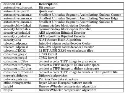
To assess the proposed methodology, we have used two major benchmark suites separately: i)cBench[Fursin 2010] and ii)PolyBench[Grauer-Gray et al. 2012; Pouchet 2012]. Each con-sists of different classes of applications and kernels ranging from security and cryptography

2_{This is by construction due to the initialization of the MWST and the K2 algorithms used to discover the network}

(12)

algorithms to office and image-processing applications. Readers can refer to Table I for the list of applications selected in the two benchmark suites.

Table I: Benchmark suites used in this work

(a)cBenchapplications selected for this work

cBench list Description

automotive bitcount Bit counter automotive qsort1 Quick sort

automotive susan c Smallest Univalue Segment Assimilating Nucleus Corner automotive susan e Smallest Univalue Segment Assimilating Nucleus Edge automotive susan s Smallest Univalue Segment Assimilating Nucleus S security blowfish d Symmetric-key block cipher Decoder

security blowfish e Symmetric-key block cipher Encoder security rijndael d AES algorithm Rijndael Decoder security rijndael e AES algorithm Rijndael Encoder security sha NIST Secure Hash Algorithm telecom adpcm c Intel/dvi adpcm coder/decoder Coder telecom adpcm d Intel/dvi adpcm coder/decoder Decoder telecom CRC32 32 BIT ANSI X3.66 crc checksum files consumer jpeg c JPEG kernel

consumer jpeg d JPEG kernel

consumer tiff2bw convert a color TIFF image to grey scale consumer tiff2rgba convert a TIFF image to RGBA color space consumer tiffdither convert a TIFF image to dither noisespace

consumer tiffmedian convert a color TIFF image to create a TIFF palette file network dijkstra Dijkstra’s algorithm

network patricia Patricia Trie data structure office stringsearch1 Boyer-Moore-Horspool pattern match bzip2d BurrowsWheeler compression algorithm bzip2e BurrowsWheeler compression algorithm

(b) Linear-algebra/applications of thePolyBenchsuite selected

for this work

PolyBench list Description

2mm 2 Matrix Multiplications (D=AB; E=CD) 3mm 3 Matrix Multiplications (E=AB; F=CD; G=EF) atax Matrix Transpose and Vector Multiplication bicg BiCG Sub Kernel of BiCGStab Linear Solver cholesky Cholesky Decomposition

doitgen Correlation Computation gemm Matrix-multiply C = AB + C

gemver Vector Multiplication and Matrix Addition gesummv Scalar, Vector and Matrix Multiplication mvt Matrix Vector Product and Transpose symm Symmetric matrix-multiply syr2k Symmetric rank2k operations syrk Symmetric rankk operations trisolv Triangular solver

trmm Triangular matrix-multiply

4.1.1. cBench.ThecBenchsuite [Fursin 2010] is a collection of open-source programs with multiple data sets assembled by the community to enable realistic workload execution and targeted by many different compilers such asGCC, LLVM, etc.. The source code of individual programs is simplified to facilitate portability; therefore, it has been targeted inautotuning

anditerative compilationresearch work. Of the available data sets for every individual kernel, we have selected five and sorted them in a way that dataset1 is always the smallest and dataset5 the largest. This ensures that for every kernel we have exposed enough of the input load to be able to measure fair runtime executions.

(13)

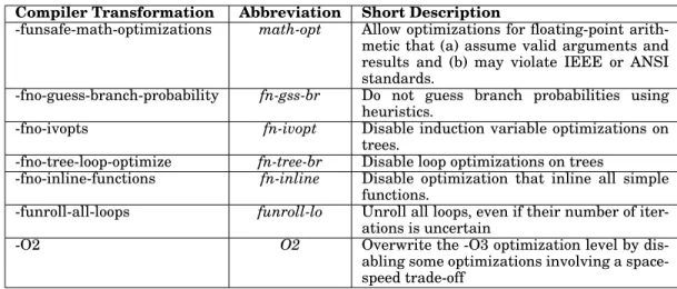
Table II: Compiler optimizations under analysis (beyond -O3) Compiler Transformation Abbreviation Short Description

-funsafe-math-optimizations math-opt Allow optimizations for floating-point arith-metic that (a) assume valid arguments and results and (b) may violate IEEE or ANSI standards.

-fno-guess-branch-probability fn-gss-br Do not guess branch probabilities using heuristics.

-fno-ivopts fn-ivopt Disable induction variable optimizations on

trees.

-fno-tree-loop-optimize fn-tree-br Disable loop optimizations on trees

-fno-inline-functions fn-inline Disable optimization that inline all simple

functions.

-funroll-all-loops funroll-lo Unroll all loops, even if their number of iter-ations is uncertain

-O2 O2 Overwrite the -O3 optimization level by

dis-abling some optimizations involving a space-speed trade-off

4.1.2. PolyBench.The PolyBench benchmark suite [Pouchet 2012; Grauer-Gray et al. 2012] consists of benchmarks with static control parts. The purpose is to make the execution and monitoring of applications uniform. One of the main features of thePolyBenchsuite is that there is a single file per application, tunable at compile-time and used for kernel instrumen-tation. It performs extra operations such as cache flushing before the execution, and can set real-time scheduling to prevent OS interference. We have defined two different data sets for each individual application to expose the main function with different input loads. PolyBench has a variety of benchmarks, i.e. 2D and 3D matrix multiplication, vector decomposition, etc.. This suite is also suitable for parallel programming, which is beyond the focus of this work. 4.2. Compiler Transformations

The compiler transformations analyzed have been reported in Table II. We based our design space on the work of [Chen et al. 2012]. The authors implemented sensitivity analysis over a vast majority of the compiler optimizations and defined with a list of promising passes. Build-ing upon their work, we selected the compiler optimizations with a speedup factor greater than 1.10. They are applied to improve application performance beyond the standard optimization level -O3 and have not yet been included in any prior optimization level. The optimizations can be enabled/disabled by means of the respective compiler optimization flags. The standard optimization level -O3 has been also used to collect the dynamic software-features for each application on bothtrainingandinferencephases.

The application execution time has been estimated by using the Linux-perf tool. The execu-tion time is done by averaging five loop-wraps of the specific compiled binary with one second of sleep in between five different executions of those loop-wraps. Therefore, in total, each in-dividual transformed binary has been executed 25 times as five packages of five loop-wraps to ensure better accuracy of estimations and fairness among the generation of executions. This technique is used both in thetrainingand theinferencephases.

4.3. Bayesian Network Results

In this work, Matlab environment [Murphy 2001; Santana et al. 2010] has been used to train the Bayesian Network. We have usedExploratory Factor Analysis (EFA) of application fea-tures for the seven compiler optimization flags listed in Table II. As stated in Section 3.2, one of the features of using EFA is that the factors are linear combinations that maximize the shared portion of the variance. Therefore, as prerequisite, the covariance matrix should be

(14)

Table III: Kaiser test results Application Characterization Method Original No. of Factors Range of Selected Factors By Kaiser Test

cBench MICA (Dynamic) 99 [7-11]

cBench MILEPOST (Static) 53 [4-6]

cBench Hybrid 143 [8-10]

polyBench MICA (Dynamic) 99 [5-7]

polyBench MILEPOST (Static) 53 [4-6]

polyBench Hybrid 143 [4-5]

positive definite. This pre-processing helps purify the highly correlated application character-ization columns that are linearly correlated. In theory,PCAaccepts any matrix ignoring the aforementioned condition and that is why we think applying factor analysis as our dimension reduction technique tends to obtain the most important factors and correlate them with the compiler optimizations. Decision on the numbers of factors have been derived from theKaiser

test [Kaiser 1958]. This test implies taking only the factors having greater than 1 in the co-variance matrix. In other words, the Kaiser rule is to drop all components with eigenvalues under 1, this being the eigenvalue equal to the information accounted for by an average single item. Table III reports the factors derived for each individual benchmark and characterization method.

Table III represents the number of features that have been produced both originally by the different feature selection techniques and by the Kaiser test. The third column is theoriginal number of featuresand the last one refers torange of selected factorsin each specific bench-mark suite/feature selection method. Note that the last column reports the range of selected factors rather than a number as we have used cross-validation approach in the experimen-tal campaign, thus different applications/datasets/feature selection techniques can result in a different number of factors to be used in COBAYN’s framework.

In this work, while training has been carried out using each application/dataset pair sep-arately, the validation has been done through an application-level cross-validation ( Leave-One-Out cross-validation, LOO). We train different BNs, each by excluding an applications (together with all its input dataset) from the training set.

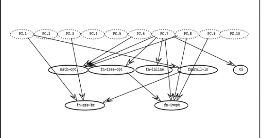
UsingBNenables us to investigate graphically the dependencies between the variables in-volved in the compiler optimization problem and to correlate them with the selected factors of the program characterization. We train a finalBayesian Networkincluding all applications in the training set. The resulting network topology is a directed acyclic graphDAG, as shown in Figure 3. By removingsecurity rijndael eapplication from the training set, the graph topology slightly changes, mainly in terms of the different edges connecting thePrincipal Components (PC)/program factors (FA)nodes to the compiler optimization nodes. This is due to the change in the program features and its factors, which are computed in a different way. For the sake of conciseness, we do not report all graph topologies derived by the LOO technique for each individual trainedBayesian Network.

The Nodes of the topology graph reported in Figure 3 are organized in layers. The first layer reports the FAs that are the observable variables (reported as dashed lines). The second layer contains the compiler optimizations whose parents are the PC nodes (or FA nodes depending weather PCA or EFA is used). Therefore the effects of these compiler optimizations depend only on the application characterization in terms of its features. In the third layer, the compiler optimization nodes whose parents include optimization nodes from the second layer are listed. Once a new application is characterized for a target application data set, the evidence related to the PCs (or FAs) of its features is fed to the network in the first layer. Then, the probability

(15)

PC.1 PC.2 PC.3 PC.4 PC.5 PC.6 PC.7 PC.8 PC.9 PC.10

math−opt

fn−gss−br fn−ivopt

fn−tree−opt fn−inline funroll−lo O2

Fig. 3: Topology of theBayesian Networkifsecurity rijndael eis left out of the training set distributions of other nodes can be inferred in turn on the second and third layers. There are two nodes in the third layer of Figure 3. The first one is the fn-gss-brnode that depends on

funroll-lo because unrolling loops impacts the predictability of the branches implementing these loops. Moreover,funroll-loimpacts the effectiveness of the heuristic branch probability estimation, thus fn-gss-br. The second node in the third layer is the fn-ivopt node, which depends onfn-tree-optas parent node in the second layer. Both these optimizations work on trees and therefore their effects are interdependent. While sampling compiler optimizations from theBayesian Network, the decisions of whether to applyfn-gss-brandfn-ivoptare taken after deciding whether to applyfunroll-loandfn-tree-opt.

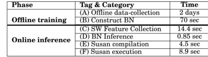
Table IV shows the fine-grain breakdown of the timing when we use COBAYN framework. We have reported the time spent for each phase of the proposed technique, both on the train-ing phase (done offline) and on the inference phase (done online). Constructtrain-ing COBAYNs network is a one-time process and depends on the number of applications in the training set. The time needed to collect the training data is on the other side, dependents not only on the number but also on the applications and data-set used for the training. The same happens for the time needed for compiling and executing the target application during the online com-piler autotuning phase. To that end, Table IV reports the numbers for each specific phase considering the cBench as training set and Susan as target application. During the offline training-phase, the time needed for data collection on the case of cBench, is around 2 days. It includes the time needed for each benchmark to compile and execute, considering all set of configuration and the feature collection phase. The time needed to post-process the data and to generate the Bayesian Network model is around 70 seconds.

During the online phase (inference phase), the time needed for extracting the software fea-tures from the target application is 14.4 seconds while, querying BN is less than 1 second. The compilation and execution-time on the target platform for Susan are 4.5 and 8.9 seconds, respectively. Those numbers show that the initial overhead in adopting the proposed method-ology on the user-side (composed of the software feature extraction and BN inference) is less than 2 compilation/executions pairs, for this specific example.

4.4. Comparison Results

It is well known that Random Iterative Compilation (RIC) can improve application perfor-mance compared with static handcrafted compiler optimization sequences [Agakov et al. 2006]. Additionally, given the complexity of the iterative compilation problem, it has been proved that drawing compiler optimization sequences at random is as good as applying other

(16)

Table IV: COBAYN timing breakdown for offline training and online inference forSusan ap-plication

Phase Tag & Category Time

Offline training

(A) Offline data-collection 2 days

(B) Construct BN 70 sec

Online inference

(C) SW Feature Collection 14.4 sec

(D) BN Inference 0.85 sec

(E) Susan compilation 4.5 sec

(F) Susan execution 8.9 sec

Table V: COBAYN (BN using EFA) speedup w.r.t standard optimization levels (-O2 and -O3) andRandom Iterative Compilation(RIC) and our previous approach of BN in [Ashouri et al. 2014] using PCA

Benchmarks Features COBAYN Speedupw.r.t

-O2 -O3 RIC BN w/ PCA

cBench Dynamic 1.6093 1.528 1.2029 1.0744 cBench Static 1.5447 1.478 1.1143 1.0543 cBench Hybrid 1.5858 1.5066 1.2086 1.0654 cBench Average 1.5795 1.5035 1.1743 1.0617 PolyBench Dynamic 1.9845 1.8387 1.3230 1.0921 PolyBench Static 1.9353 1.8215 1.1518 1.0724 PolyBench Hybrid 1.9441 1.7726 1.2333 1.1078 PolyBench Average 1.9541 1.8101 1.2350 1.0901

Overall (Harmonic Mean) 1.7669 1.6571 1.2052 1.0771

optimization algorithms such as genetic algorithms or simulated annealing [Agakov et al. 2006; Cavazos et al. 2007; Chen et al. 2012]. Accordingly, to evaluate the proposed approach, we compared our results withi) standard optimization levels -O2 and -O3 ii) the Random Iterative Compilation (RIC) methodology that samples compiler optimization sequences from the uniform distribution andiii)two advanced state-of-the-art methodologies, namelya) (Sec-tion 4.6.1) coupling machine learning with an iterative methodology, andb) (Section 4.6.2) a non-iterative methodology derived bypredictive modelingbased on different machine-learning algorithms to predict the final application speedup.

The proposed methodology samples different compiler optimization sequences from the BN. The performance achieved by the best application binary depends on the number of sequences sampled from the model. In this section, the result of applying the proposed methodology using two benchmark suites with respect to standard optimization levels and therandom iterative compilationhave been reported. The performance speedup on the first comparison section is measured in reference to -O2 and -O3, which are the optimization levels available for GCC. In addition, we show the speedup of the proposed methodology with respect to our previous work [Ashouri et al. 2014].

4.4.1. Bayesian Networks Performance Evaluation.Table V reports COBAYN’s speedup achieved over the standard optimization levels of-O2and-O3andRandom Iterative Compilation (RIC). The last column represents the average speedup achieved by revising ourBayesian Network

engine and using theExplanatory Factor Analysis (EFA)described in the Section 3.2 with re-spect to PCA in [Ashouri et al. 2014]. Note that all speedup values have been averaged using Harmonic mean. It is observed that in all categories, COBAYN outperforms standard opti-mization levels and the previous approach. The comparison with respect to the RIC has been

(17)

1 1.5 2 2.5 3 consumer jpeg d automotive bitcount consumer tiffmedian

telecom adpcm c consumer jpeg c security blowfish e automotive susan s

telecom adpcm d automotive qsort1 consumer tiff2rgba automotive susan c

bzip2d telecom CRC32

bzip2e

automotive susan e _{security rijndael e}_{security rijndael d}_{security blowfish d} office stringsearch1

consumer tiff2bw consumer tiffdither

security sha network dijkstra network patricia

Performance improvement w.r.t

-O3 and -O2

w.r.t -O2 w.r.t -O3

(a) BN with dynamic features on cBench

1 1.5 2 2.5 3 3.5 4 4.5 gemm 3mm 2mm doitgen atax

trisolv syr2k bicg cholesky

trmm symm gemver mvt gesummv syrk Performance improvement w.r.t

-O3 and -O2

w.r.t -O2 w.r.t -O3

(b) BN with dynamic features on PolyBench

1 1.5 2 2.5 3 automotive bitcount consumer jpeg c consumer tiffmedian consumer jpeg d telecom adpcm c

security blowfish e automotive susan s automotive qsort1 bzip2d

consumer tiff2rgba telecom adpcm d

security rijndael d automotive susan c bzip2e telecom CRC32 automotive susan e security rijndael e _{office stringsearch1}

consumer tiff2bw security blowfish d consumer tiffdither

-O3 and -O2

w.r.t -O2 w.r.t -O3

(c) BN with static features on cBench

1 1.5 2 2.5 3 3.5 4 4.5 gemm 3mm 2mm

doitgen syr2k atax symm _{cholesky trisolv}

bicg syrk trmm gemver

mvt gesummv

-O3 and -O2

w.r.t -O2 w.r.t -O3

(d) BN with static features on PolyBench

1 1.5 2 2.5 3 consumer jpeg d automotive bitcount consumer tiffmedian

telecom adpcm c consumer jpeg c security blowfish e automotive qsort1 automotive susan s

bzip2d

security rijndael e automotive susan c telecom adpcm d telecom CRC32

security rijndael d consumer tiff2rgba bzip2e

automotive susan e consumer tiff2bw _{security blowfish d} office stringsearch1 consumer tiffdither

-O3 and -O2

w.r.t -O2 w.r.t -O3

(e) BN with dynamic+static features on cBench

1 1.5 2 2.5 3 3.5 4 4.5 gemm 3mm 2mm doitgen trisolv atax bicg cholesky

syr2k syrk symm trmm mvt

gesummv gemver

-O3 and -O2

w.r.t -O2 w.r.t -O3

(f) BN with dynamic+static features on PolyBench

(18)

Table VI: Evaluation of different BigSet formation in COBAYN Model Construction. Note that COBAYN’s default refers to the version of COBAYN trained on a single benchmark set.

BigSet Combination Speedup w.r.t. COBAYN’s Default cBench PolyBench 24 (All) 15 (All) 1.1143 15 15 1.0743 10 10 1.0432 5 5 0.9896

reported by the Harmonic average over the speedup data derived by dividing the COBAYN’s performance data by the RIC data in full space. It can be seen that dynamic feature selec-tion brings best results followed by the hybrid and static method. However, in certain cases (cBench using hybrid SW features), it narrowly reaches the performance of dynamic feature selection.

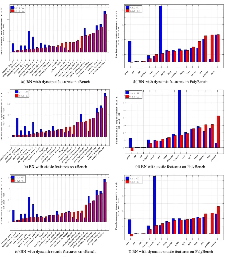
Using two major benchmarks and three different application characterization techniques, we report six different plots showcasing the benefits of the proposed methodology with respect to the GCC standard optimization levels. Figure 4, reports the speedups by considering a sam-ple of eight different compiler optimization sequences. For each benchmark, the results have been averaged on the different data sets. All results have been sorted by the speedup values of -O3 and have been matched with their corresponding -O2 value. The bar plot is colored in blue and red, respectively, for the speedup achieved with respect to -O2 and -O3. All applications have achieved a speedup in reference to the performance of -O2 and -O3. This happens with the exception ofgemm in reference to -O3 for static and hybrid feature-selection techniques andconsumer-jpeg-din reference to -O3 when using the dynamic method for feature selection. These applications reach their best performance using -O3 for two data sets out of five, and it was not possible to surpass this maximum by relying on the compiler transformations under consideration. On average forcBench, the speedups are of1.57and1.5in reference to -O2 and -O3, respectively, and1.95and1.81forPolyBench. The maximum speedup observed is3.1×

and4.7×. Table V reports the speedup gained using COBAYN compared with the standard op-timization levels,Random Iterative Compilation (RIC)and our previous approach exploiting

PCAas dimension-reduction method.

Analysis of the Portability of COBAYN in Different Scenarios.The results reported in this section are computed by means of LOO cross-validation on the two individual benchmark suites separately, one with 24 and the other with 15 applications. As the nature of these two benchmark suites is totally different, we believed it would be unfair to train on one and test on the other, so we analyzed the feasibility of mixing these applications in a fair heteroge-neous set ofBigSetso that COBAYN’s engine gets evaluated. To this end, we tried 4 different scenarios, where the BigSet is obtained by: (i) including all 39 available applications, (ii) 15 applications of cBench and 15 applications of PolyBench, (iii) selecting 10 cBench and 10 Poly-Bench and finally (iv) 5 applications from each of those. Therefore, the BigSet was initialized with 39, 30, 20 and 10 different applications, and LOO cross-validation was carried-out. Ta-ble VI reports the speedup gained in these scenarios. It is observed that COBAYN framework benefits from havinga)more applications, andb)heterogeneous applications in the training set. The speedup listed in Table VI is higher when BigSet accounts for more applications and, even just 10 applications per benchmark suite, it is higher than one (the default setting for the experimental results in this work refers to the COBAYN trained only on one of the two benchmark suites).

4.4.2. Performance Improvement.Let us define theNormalized Performance Improvement(NPI) as the ratio of the performance improvement achieved over the potential performance im-provement:

(19)

N P I= Eref −E

Eref −Ebest

(1) whereE is the execution time achieved by the methodology under consideration,Eref is the

execution time achieved with a reference compilation methodology andEbest is the best

exe-cution time computed through an exhaustive exploration of all possible compiler optimization sequences (in our case 128 different sequences). As the execution timeEof the iterative com-pilation methodology under analysis gets closer to the reference execution timeEref, the NPI

gets closer to 0, reporting that no improvement is returned. In the same way, asEgets closer to the best execution timeEbest, while NPI gets close to 1, reporting that the entire potential

performance improvement has been achieved.

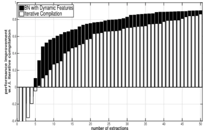
Figure 5 reports for six different benchmark/feature selection methods; the NPI achieved by theproposed optimizationtechnique and by the RIC technique in reference to the execution time obtained by -O3 (Eref ). It is noticeable that NPI has the upper-hand on performance

on every number of extractions with respect to RIC. For readability purposes, we have only reported the first 50 extraction of the design space. The trend is continuously applied to the rest of the extractions until both get the maximum performance value of 1 at extraction no. 128, which accounts for the optimal compiler sequence given the specific application (also it is the optimal performance using exhaustive search). The comparisons reported in Figure 5 were carried out by considering the same number of compiler optimization sequences sampled for both the RIC and theproposedapproach. We acknowledge the fact that there is still room for improvement in future work. However, NPI figures show that in all cases, the proposed method was superior in terms of performance and that 30 extractions, on the current scale, reach 80%of the optimality.

4.5. A Practical Usage Assessment

When usingiterative compilationin realistic cases, we need to decide how much effort should be spent on the optimization itself. This effort can be measured in terms of optimization time, which is directly proportional to the number of compilations to be executed. Thus, in this sec-tion, we evaluate the proposed optimization approach in terms of the application performance reached after a fixed number of compilations. In particular, we fix this number to eight which represents 6.25% of the overall optimization space. Our model has been compared with RIC and in Figure 6, we report theviolinplot for application speedup, while keeping the compila-tion effort of the proposed methodology to eight compilacompila-tions (or extraccompila-tions) and varying the compilation efforts of the RIC to explore more compiler space in the long run. Each individ-ual distribution in Figure 6 represents the performance of the proposed work with respect to

RICacross different extractions. The red cross marks themeanand the green square marks the median of each violin distribution. It can be seen that the proposed methodology with BN inference achieved an at least 3×reduction in exploration process effort compared with the same extraction of RIC. Here we defineexploration speedupas the factor measuring the aforementioned metrics, enabling the researchers to traverse the compiler design space more efficiently.

Accordingly, by increasing the compilation efforts on RIC, while keeping the exploration efforts of the proposed approach constant, the application speedup of COBAYN decreases. On average, RIC needs 24-32 extractions to achieve the application performance obtained with eight extractions by COBAYN. This means that COBAYN provides a speedup of 3-4×in terms of optimization efforts, that is only slightly impacted by the initial overhead (less than 2 evaluations) reported in Section 4.3. Furthermore, at the most extreme case, when RIC exhaustively enumerates and explores the full-space, 8 extractions of COBAYN, on average, still could gain up to 91% of the optimal solution. This is shown on the final distribution of eachviolinplot separated by a vertical dashed-line.

(20)

number of extractions

0 5 10 15 20 25 30 35 40 45 50

performance improvement w.r.t. iterative compilation

-0.4 -0.2 0 0.2 0.4 0.6 0.8 1

BN with Dynamic Features Iterative Compilation

0 5 10 15 20 25 30 35 40 45 50

-0.4 -0.2 0 0.2 0.4 0.6 0.8 1

BN with Dynamic Features Iterative Compilation

0 5 10 15 20 25 30 35 40 45 50

-0.4 -0.2 0 0.2 0.4 0.6 0.8 1

BN with Static Features Iterative Compilation