SOUND INTENSITY AND ITS
MEASUREMENT AND APPLICATIONS
Finn Jacobsen
Acoustic Technology, Department of Electrical Engineering Technical University of Denmark, Building 352
Ørsteds Plads, DK-2800 Lyngby Denmark
fja@elektro.dtu.dk
CONTENTS
Page
1 Introduction . . . 5
2 Sound fields, sound energy and sound intensity . . . 6
2.1 Conservation of sound energy . . . 6
2.2 Other important relations . . . 9
2.3 Active and reactive sound intensity . . . 11
3 Measurement of sound intensity . . . 15
3.1 Measurement principles . . . 15
3.2 Errors and limitations . . . 17
3.3 Testing and verification . . . 23
4 Applications . . . 24
References . . . 27
Bibliography . . . 30
List of symbols . . . 31
Appendix A: Complex notation . . . 33
Appendix B: Levels and decibels . . . 35
Appendix C: Standards for sound intensity measurements . . . 37
1. INTRODUCTION
The most important acoustic quantity is the sound pressure, which is an acoustic first-order quantity. However, sources of sound emit sound power, and sound fields are also energy fields in which potential and kinetic energies are generated, transmitted and dissipated. In spite of the fact that the radiated sound power is a negligible part of the energy conversion of almost any sound source, energy considerations are of enormous practical importance in acoustics. In ‘energy acoustics’ sources of noise are described in terms of their sound power, acoustic materials are described in terms of the fraction of the incident sound power that is absorbed, and the sound insulation of partitions is described in terms of the fraction of the incident sound power that is transmitted, the underlying assumptions being that these properties are independent of the particular circumstances. None of these assumptions is true in the strict sense of the word. However, they are usually good approximations in a significant part of the audible frequency range, and alternative methods based on linear quantities are vastly more complicated than the simple energy balance considerations of energy acoustics.
Sound intensity is a measure of the flow of acoustic energy in a sound field. More precisely, the sound intensity I is a vector quantity defined as the time average of the net flow of sound energy through a unit area in a direction perpendicular to the area. The dimensions of the sound intensity are energy per unit time per unit area (W/m2). Although acousticians have
attempted to measure this quantity since the 1930s, the first reliable measurements of sound intensity under laboratory conditions did not occur until the middle of the 1970s. Commercial sound intensity measurement systems came on the market in the beginning of the 1980s, and the first international standards for measurements using sound intensity and for instruments for such measurements were issued in the middle of the 1990s. A description of the history of the development of sound intensity measurement is given in Fahy’s monograph Sound Intensity (see the bibliography).
The advent of sound intensity measurement systems in the1980s has had a significant influence on noise control engineering. Sound intensity measurements make it possible to determine the sound power of sources without the use of costly special facilities such as anechoic and reverberation rooms, and sound intensity measurements are now routinely used in the determination of the sound power of machinery and other sources of noise in situ. Other important applications of sound intensity include the identification and rank ordering of partial noise sources, visualisation of sound fields, determination of the transmission losses of partitions, and determination of the radiation efficiencies of vibrating surfaces.
The sound intensity method is not without problems, though. Some people consider the method very difficult to use, and it cannot be denied that more knowledge is required in measuring sound intensity than in, say, using an ordinary sound level meter. The difficulties are mainly due to the fact that the accuracy of sound intensity measurements with a given measurement system depends very much on the sound field under study. Another problem is that the distribution of the sound intensity in the near field of a complex source is far more complicated than the distribution of the sound pressure, indicating that sound fields can be much more complicated than earlier realised. The problems are reflected in the extensive literature on the errors and limitations of sound intensity measurement and in the fairly complicated international and national standards for sound power determination using sound intensity, ISO 9614-1, ISO 9614-2, ISO 9614-3 and ANSI S12.12.
The purpose of this note is to give a brief but nevertheless relatively detailed overview of sound intensity and its measurement and applications.
2. SOUND FIELDS, SOUND ENERGY AND SOUND INTENSITY
It can be shown [1] that the instantaneous potential energy density in a sound field (the potential sound energy per unit volume) is given by the expression
(2.1) where p(t) is the sound pressure as a function of time, D0 is the equilibrium density of the
medium, and c is the speed of sound. This quantity describes the energy stored in a unit volume of the medium because of compression or rarefaction; the phenomenon is analogous to the potential energy in a compressed or elongated spring.
The instantaneous kinetic energy density in a sound field (the kinetic energy per unit volume) is [1, 2]
(2.2) where u(t) is the magnitude of the particle velocity vector u(t). This quantity describes the energy per unit volume represented by the moving mass of the particles of the medium.
The instantaneous sound intensity is the product of the sound pressure and the particle velocity,
(2.3) This quantity, which is a vector, expresses the magnitude and direction of the instantaneous flow of sound energy per unit area, as shown in the following.
2.1 Conservation of sound energy
The divergence of the instantaneous sound intensity I(t) is
(2.4)
If we combine the linearised equation of conservation of mass,
(2.5) where D is the instantaneous density of the medium, with the adiabatic relation between changes in the sound pressure and in the density,
(2.6) we can derive a relation between the divergence of the particle velocity and the rate of change of the sound pressure, needed in evaluating the first term of the right-hand side of eq. (2.4):
1The derivation based on the linarised acoustic equations (2.5), (2.6) and (2.7) is due to Kirchhoff.
Strictly speaking the acoustic energy corollary (eq. (2.10)) should be derived on the basis of the full, non-linear equations rather than the linearised equations, and afterwards reduced to second order. However, since various terms cancel out the result is the same [1-3].
(2.7)
To calculate the second term we need Euler’s equation of motion (conservation of momentum), (2.8) Inserting eqs. (2.7) and (2.8) into eq. (2.4) gives
(2.9) For simplicity, the equilibrium density has here and in what follows been written as Drather than
D0. The quantity in the right-hand parenthesis is recognised as the sum of the instantaneous
potential energy density and the instantaneous kinetic energy density, so all in all it can be concluded that
(2.10) where w(t) is the total instantaneous energy density.1 This is the equation of conservation of
sound energy, which expresses the simple fact that the rate of decrease of the sound energy density at a given position in a sound field (represented by the right-hand term) is equal to the rate of the flow of sound energy diverging away from the point (represented by the left-hand term).
That eq. (2.10) represents a conservation law is perhaps easier to see from the global version. This is obtained using Gauss’s theorem, according to which the net outflow of sound energy integrated over a given volume equals the total net outflow of sound energy through the surface of the volume,
(2.11) where S is the area of a surface around the source and V is the volume contained by the surface. Combining with eq. (2.10) gives
(2.12) which shows that the total net outflow of sound energy through the surface equals the (negative) rate of change of the total sound energy within the surface, E. In other words, the rate of change of the sound energy within a closed surface is identical with the surface integral of the normal
component of the instantaneous sound intensity, I(t).
In practice we are often concerned with the time-averaged sound intensity in stationary sound fields. For simplicity we use the symbol I for this quantity (rather than ), that is,
(2.13) where the bar indicates averaging with respect to time. Examination of eq. (2.10) leads to the conclusion that the divergence of the time averaged sound intensity is identically zero,
(2.14) and that the time-average of the instantaneous net flow of sound energy out of a given closed surface is zero unless there is generation or dissipation of sound power within the surface, that is,
(2.15) irrespective of the presence of sources outside of the surface. If the surface encloses a steady sound source that radiates the sound power Pa then the time-average of the net flow of sound energy out of the surface is equal to the net sound power of the source, that is,
(2.16) irrespective of the presence of other steady sources outside the surface and irrespective of the shape of the surface. This important equation is the basis of sound power determination using sound intensity.
Example 2.1
If we add a source term corresponding to monopole with the volume velocity Q at the position r0 to the
right-hand side of eq. (2.5) it becomes
(see, e.g., refs. [4, 5]). Combining with eqs. (2.4), (2.6) and (2.8) gives
and when this is integrated over a volume and use is made of Gauss’s theorem the result is
when r0 is outside the closed integration surface and
when r0 is inside the surface. If the monopole is emitting a stationary signal averaging over time gives
2In this note a tilde over a symbol indicates a harmonic variable in complex notation. 3As shown in Appendix B eq. (2.20) also implies that L
I•Lp under normal ambient conditions. Example 2.2
In a sound field generated by two sources we can write and
(linear superposition), from which it follows that
Note that when the sources are uncorrelated the two sound intensity vectors are simply added, since the time average of each cross term is zero. However, this is not the case when the sources are correlated.
2.2 Other important relations
If the sound field is harmonic with angular frequency T = 2Bf we can make use of the usual complex representation of the sound pressure and the particle velocity,2
(2.17a, 2.17b)
(For simplicity we consider only the component of the particle velocity in the r-direction here.) Expressed in terms of these quantities eq. (2.13) becomes
(2.18) where denotes the complex conjugate of , and n is the phase angle between the sound pressure and the particle velocity (see Appendix A).
In a plane progressive wave the sound pressure and the particle velocity are in phase (n
= 0) and related by the characteristic impedance of the medium, Dc:
(2.19) Thus for a plane wave the sound intensity is
(2.20) In this case the sound intensity is simply related to the mean square sound pressure which can be measured with a single microphone.3 Equation (2.20) is also valid in the simple spherical
sound field generated by a monopole source in free space, irrespective of the distance to the source. However, in the general case the sound intensity is not simply related to the sound pressure, and both the sound pressure and the particle velocity must be measured simultaneously and their instantaneous product time-averaged. This requires the use of a more complicated device than a single microphone.
Example 2.3
The divergence of the time averaged sound intensity can be written
Expressed in complex notation eqs. (2.7) and (2.8) become
and
When these two equations are inserted into the expression for the divergence of I eq. (2.14) results.
Example 2.4
Adding a source term corresponding to a harmonically varying monopole with the volume velocity Q at the position r0 to the right-hand side of the expression for the divergence of the particle velocity gives
(cf. example 2.1). The divergence of the time averaged sound intensity now becomes ,
and the integral over a volume closed by the surface S becomes
Example 2.5
In a simple spherical sound field we have the following relation between the sound pressure and the particle velocity,
It is apparent that the component of the particle velocity in phase with the sound pressure is just as in a plane propagating wave, which explains why the sound intensity equals
Example 2.6
The free-field method of estimating the sound power of a source relies on the fact that the plane wave expression for the sound intensity, eq. (2.20), is a good approximation sufficiently far from any finite source in free space (the sound field becomes ‘locally plane’). In practice an anechoic room is required.
For later reference we will derive a relation between the sound intensity and the gradient of the phase of the sound pressure in a harmonic sound field. If we write the complex sound pressure in the form of an amplitude and a phase,
(2.21) and make use of Euler’s equation of motion, eq. (2.8), then the expression for the sound intensity becomes
(2.22)
which shows that the sound intensity equals the product of and the gradient of the phase of the sound pressure normalised with the wavenumber. Inspection of this equation leads to the interesting conclusion that the time-averaged sound intensity is orthogonal to the wavefronts, that is, surfaces of constant phase in the sound field [6].
Example 2.7
The sound pressure at a distance r from a monopole point source with volume velocity Q is
Note that the gradient of the phase in the r-direction equals - k, just as in a plane propagating sound wave. Inserting in eq. (2.22) shows that
cf. example 2.5.
2.3 Active and reactive sound intensity
In spite of the diversity of sound fields encountered in practice, some typical sound field characteristics can be identified. For example, the sound field far from the source that generates it has certain well-known properties under free-field conditions, the sound field near a source has other characteristics, and some characteristics are typical of a reverberant sound field, etc.
We have seen that the sound pressure and the particle velocity are in phase in a plane propagating wave. This is also the case in a free field, sufficiently far from the source that generates the field. Conversely, one of the characteristics of the sound field near a source is that the sound pressure and the particle velocity are partly out of phase (in quadrature). To describe such phenomena one may introduce the concept of active and reactive sound fields.
It takes four second-order quantities to describe the distributions and fluxes of sound energy in a sound field completely [6-8]: potential energy density, kinetic energy density, active intensity (which is the quantity we usually simply refer to as the intensity), and reactive intensity. The last mentioned of these quantities represents the non-propagating, oscillatory sound energy flux that is characteristic of a sound field in which the sound pressure and the particle velocity are in quadrature, as for instance in the near field of a small source. The reactive intensity is a vector defined as the imaginary part of the product of the complex pressure and the complex conjugate of the particle velocity,
(2.23) (cf. eq. (2.18)). More general time-domain formulations based on the Hilbert transform are also available [8]. Unlike the usual active intensity, the reactive intensity remains a somewhat controversial issue although the quantity was introduced in the middle of the previous century
[9], perhaps because the vector J has no obvious physical meaning [10], or perhaps because describing an oscillatory flux by a time-averaged vector seems peculiar to some. However, even though the reactive intensity is of no obvious direct practical use it nevertheless is quite convenient that we have a quantity that makes it possible to describe and quantify the particular sound field conditions in the near field of sources in a precise manner.
Very near a sound source the reactive field is usually stronger than the active field. However, the reactive field dies out rapidly with increasing distance to the source. Therefore, even at a fairly moderate distance from the source, the sound field is dominated by the active field. The extent of the reactive field depends on the frequency, and the dimensions and the radiation characteristics of the sound source. In practice, the reactive field may be assumed to be negligible at a distance greater than, say, half a metre from the source.
Figure 2.1 Measurement in an active sound field (from reference [11]). (a) )) , Instantaneous sound pressure; - - - , instantaneous particle velocity multiplied by Dc. (b) Instantaneous sound intensity. (c) ))) , Real part of ‘complex instantaneous intensity’; - - - , imaginary part of ‘complex instantaneous intensity’. One-third octave noise with a centre frequency of 1 kHz.
Example 2.8
From example 2.5 we can calculate the specific impedance at a distance r from a monopole:
Apparently, this quantity is almost purely imaginary when kr << 1, indicating that the sound pressure and the particle velocity are nearly 90° out of phase in the nearfield of the source. Note that the specific impedance is mass-like under such condition, that is, proportional to jT, in agreement with the fact that the radiation impedance of a monopole is dominated by the mass term.
Figure 2.2 Measurement in a reactive sound field (from reference [11]). Key as in figure 2.1. One-third octave noise with a centre frequency of 250 Hz.
Figures 2.1, 2.2 and 2.3 demonstrate the physical significance of the active and reactive intensities. Figure 2.1 shows the result of a measurement at a position about 30 cm (about one wavelength) from a small monopole source, a loudspeaker driven with a band of one-third octave noise. The sound pressure and the particle velocity (multiplied by Dc) are almost identical; therefore the instantaneous intensity is always positive: this is an active sound field. In figure 2.2 is shown the result of a similar measurement very near the loudspeaker (less than one tenth of a wavelength from the cone). In this case the sound pressure and the particle velocity are almost in quadrature (90° out of phase), and as a result the instantaneous intensity fluctuates about zero, that is, sound energy flows back and forth. This is an example of a strongly reactive sound field. Finally figure 2.3 shows the result of a measurement in a reverberant room several metres from the loudspeaker generating the sound field. Here the sound pressure and the particle velocity appear to be uncorrelated signals; this is neither an active nor a reactive sound field; this is a diffuse sound field.
If we combine eqs. (2.21) and (2.23) we can derive a relation between the reactive intensity and the gradient of the amplitude of the sound pressure, analogous to eq. (2.22):
(2.24)
This equation shows that the reactive intensity is orthogonal to surfaces of equal sound pressure amplitude [6].
Figure 2.3 Measurement in a diffuse sound field (from reference [11]). Key as in figure 2.1. One-third octave noise with a centre frequency of 500 Hz.
The fact that I is the real part and J is the imaginary part of has lead to the concept of complex sound intensity,
(2.25) Note the interesting relation
A ‘complex instantaneous intensity’ has also been suggested. As can be seen from figures 2.1 (c), 2.2 (c) and 2.3 (c) the real and imaginary parts of this quantity represent the envelopes of the active and reactive instantaneous intensity. See reference [11] for an overview of the various ‘sound intensities’.
3. MEASUREMENT OF SOUND INTENSITY
It is far more difficult to measure sound intensity than to measure sound pressure. One problem is that the accuracy depends strongly on the sound field under study; under certain conditions even minute imperfections of the measuring equipment will have a significant influence on the results. With hindsight the 50-year delay from Olson submitted his application for a patent for an intensity meter in 1931 to commercial measurement systems came on the market in the beginning of the 1980s is therefore not surprising. See chapter 2 in Fahy’s Sound Intensity.
3.1 Measurement principles
Attempts to develop sound intensity probes based on the combination of a pressure transducer and a particle velocity transducer have occasionally been described in the literature. For example, a device that combined a pressure microphone with a transducer based on the convection of an ultrasonic beam by the particle velocity ‘flow’ was produced by Norwegian Electronics for some years. However, the production of this device was stopped in 1993. More recently a micro-machined transducer based on hot wire technology, ‘Microflown’, has become available for measurement of particle velocity. A sound intensity probe based on this transducer combined with a small pressure microphone is in commercial production [12, 13], and results seem to indicate that it has potential [14]. However, one problem with any particle velocity transducer, irrespective of the measurement principle, is the strong influence of airflow. Another problem is how to determine the phase correction that is needed when two fundamentally different transducers are combined. Several possible methods are described in reference [15].
All sound intensity measurement systems in commercial production today except the Microflown are based on the ‘two-microphone’ (or ‘p-p’) principle, which makes use of two closely spaced pressure microphones and relies on a finite difference approximation to the sound pressure gradient, and the IEC 1043 standard on instruments for the measurement of sound intensity, which was published in 1993, deals exclusively with the p-p measurement principle. Accordingly, all the considerations in this chapter concern this measurement principle.
The p-p measurement principle employs two closely spaced pressure microphones. The particle velocity is obtained through Euler’s relation, eq. (2.8), as
(3.1)
where p1 and p2 are the sound pressure signals from the two microphones, )r is the microphone separation distance, and J is a dummy time variable. The caret indicates the finite difference estimate, which of course is an approximation to the real sound pressure gradient. The sound pressure at the centre of the probe is estimated as
4This follows from the fact that eq. (3.3) expressed in the frequency domain has the form
where the last quation sign follows from the fact that only the imaginary part of the cross spectrum (which is an odd function
and the time-averaged intensity component in the axial direction is, from eqs. (3.1), (3.2) and (2.13),
(3.3) Some sound intensity analysers use eq. (3.3) to measure the intensity in frequency bands (one-third octave bands, for example). Another type calculates the intensity from the imaginary part of the cross spectrum of the two microphone signals, S12,
(3.4)
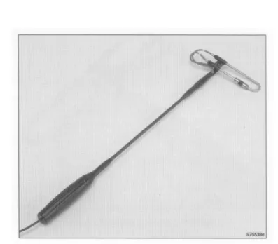
Figure 3.1 Sound intensity probe manufactured by Brüel & Kjær. The microphones are ‘face-to-face’.
The time domain formulation is equivalent to the frequency domain formulation, and in principle eq. (3.4) gives exactly the same result as eq. (3.3) when the intensity spectrum is integrated over the frequency band of concern.4 The frequency domain formulation, which makes it possible to
determine sound intensity with a dual channel FFT analyser, was derived independently by Fahy and Chung in the late 1970s [16, 17].
side’. The latter arrangement has the advantage that the diaphragms of the microphones can be placed very near a radiating surface, but the disadvantage that the microphones disturb each other. At high frequencies the face-to-face configuration with a solid spacer between the microphones is superior [18]. A face-to-face sound intensity probe produced by Brüel & Kjær is shown in figure 3.1. The ‘spacer’ between the microphones stabilises the ‘acoustic distance’ between them.
3.2 Errors and limitations in measurement of sound intensity
There are many sources of error in the measurement of sound intensity, and a considerable part of the sound intensity literature has been concerned with identifying and studying such errors. Some of the sources of error are fundamental and others are associated with various technical deficiencies. As mentioned, one complication is that the accuracy depends very much on the sound field under study; under certain conditions even minute imperfections in the measuring equipment will have a significant influence. Another complication is that small local errors are sometimes amplified into large global errors when the intensity is integrated over a closed surface, as pointed out by Pope [19].
The following is an overview of some of the sources of error in the measurement of sound intensity. Literature with more detailed discussions is listed in the bibliography.
Those who make sound intensity measurements should know about the limitations imposed by
• the finite difference error [20],
• errors due to scattering and diffraction [18, 21], and • instrumentation phase mismatch [17, 22, 23].
Airflow can be a problem, and strictly speaking the p-p measurement principle is simply not valid in a moving medium [24]. However, the resulting error is negligible if the speed of the flow is less than, say, 10 m/s. Under such conditions the main problem caused by the airflow is that the measurements are affected by
• additive ‘false’ intensity signals caused by turbulence at low frequencies [25].
A windscreen on the sound intensity probe reduces the problem of flow-induced false intensity signals, but under some circumstances
• bias errors caused by the losses of the windscreen [26] will occur.
In measurement of sound intensity at discrete points one should be aware of the • random errors associated with a given finite averaging time [27, 28],
which tend to be larger than the corresponding errors in measurement of the sound pressure, and sometimes very much larger. If the sound intensity level is low, say, less than 50 dB, one should be aware of an additional
• random error caused by electrical noise in the microphones [29], which in practice can make the measurement impossible at low frequencies.
An finally, if ordinary condenser microphones are used rather than microphones with reduced vent sensitivity [30], a
• bias error caused by the microphones pressure equalisation vent [31] can also occur.
Errors due to the finite difference approximation
The most fundamental limitation of the p-p measurement principle is due to the fact that the sound pressure gradient is approximated by a finite difference of pressures at two discrete points. This obviously imposes an upper frequency limit that is inversely proportional to the distance between the microphones. The resulting bias error depends on the sound field in a
complicated manner [20]. In a plane sound wave of axial incidence the finite difference error, that is, the ratio of the measured intensity Îr to the true intensity Ir, can be shown to be [32]
(3.5)
Figure 3.2 Finite difference error of an ideal two-microphone sound intensity probe in a plane wave of axial incidence for different values of the separation distance. ))) , 5 mm; - - -, 8.5 mm;AAAA, 12 mm; )) )) , 20 mm;
)) A )) A, 50 mm. (From reference [18].)
Figure 3.3 Error of a sound intensity probe with half-inch microphones in the face-to-face configuration in a plane wave of axial incidence for different spacer lengths. ))) , 5 mm; - - -, 8.5 mm; AAAA, 12 mm; )) )) , 20 mm;
)) A )) A, 50 mm. (From reference [18].)
This relation is shown in figure 3.2 for different values of the microphone separation distance. The upper frequency limit of intensity probes has generally been considered to be the frequency at which this error is acceptably small. With 12 mm between the microphones (a typical value) this gives an upper limiting frequency of about 5 kHz.
Errors due to scattering and diffraction
Equation (3.5) is correct for an ideal sound intensity probe that does not in any way disturb the sound field. In other words, the interference of the microphones on the sound field has been ignored. This would be a good approximation if the microphones were small compared with the distance between them, but it is not a good approximation for a typical sound intensity probe such as the one shown in figure 3.1. The high frequency performance of a real, physical probe is obviously a combination of the finite difference error and the effect of the probe itself on the sound field. In the particular case of the face-to-face configuration it turns out that the two effects to some extent cancel each other for a certain geometry; a recent numerical and experimental study has shown that the upper frequency limit of such an intensity probe can be extended to about an octave above the limit determined by the finite difference error if the length of the spacer between the microphones equals the diameter. The physical explanation is that the resonance of the cavities in front of the microphones gives rise to a pressure increase that to some extent compensates for the finite difference error. Thus the resulting upper frequency limit of a sound intensity probe composed of half-inch microphones separated by a 12-mm spacer is 10 kHz, which is an octave above the limit determined by the finite difference error when the interference of the microphones on the sound field is ignored [18]; compare figures 3.2 and 3.3. No similar serendipitous cancelling of errors occurs with the side-by-side configuration. Instrumentation phase mismatch
Phase mismatch between the two measurement channels is the most serious source of error in the measurement of sound intensity, even with the best equipment that is available today. It can be shown that the estimated intensity, subject to a phase error ne, to a very good
approximation can be written as
(3.6) that is, the phase error causes a bias error in the measured intensity that is proportional to the phase error and to the mean square pressure [22]. Equation (3.6) is a consequence of eq. (2.22) and can be derived by inserting the actual phase angle between the sound pressure signals in the sound field plus the phase error due to the measurement system into this expression. Ideally the phase error should be zero, of course. In practice one must, even with state-of-the-art equipment, allow for phase errors ranging from about 0.05/ at 100 Hz to 2/ at 10 kHz. Both the IEC standard and the North American ANSI standard on instruments for the measurement of sound intensity specify performance evaluation tests that ensure that the phase error is within certain limits.
Example 3.1
In a plane wave and in a simple spherical wave the gradient of the phase of the sound pressure in the direction of propagation equals - k (cf. example 2.7). It follows that the physical phase difference between the pressures at two points a distance of )r apart is k)r. With 12 mm between the microphones this amounts to about 3° at 250 Hz. Obviously, the phase error introduced by the measurement system should be much smaller than that, say, no larger than 0.3°. Moreover, as shown in example 3.2 the requirements are much stronger in an interference field.
Example 3.2
Equation (2.22) shows that the gradient of the phase of the sound pressure can be expressed in terms of the ratio of the mean square pressure to the sound intensity,
However, since the ratio may take values of up to, say, ten, under realistic measurement conditions it follows that the phase gradient can easily be ten times smaller than in a plane propagating wave. In other words, it is quite reasonable to require that the phase error of an intensity measurement system at 250 Hz should be much smaller than 0.3°, that is, very small indeed; cf. example 3.1.
Equation (3.6) is often written in the form
(3.7)
where the residual intensity Io and the corresponding sound pressure po,
(3.8)
have been introduced. The residual intensity is the ‘false’ sound intensity indicated by the instrument when the two microphones are exposed to the same pressure po, for instance in a small cavity. Under such conditions the true intensity is zero, and the indicated intensity Io should
obviously be as small as possible. The right-hand side of eq. (3.7) clearly shows how the error caused by phase mismatch depends on the ratio of the mean square pressure to the intensity in the sound field – in other words on the sound field condition.
Phase mismatch is usually described in terms of the so-called residual pressure-intensity index,
(3.9) which is just a convenient way of measuring, and describing, the phase error ne. With a
microphone separation distance of 12 mm the typical phase error mentioned above corresponds to a pressure-residual intensity index of 18 dB in most of the frequency range. The error due to phase mismatch is small provided that
(3.10) where
(3.11) is the pressure-intensity index of the measurement. The inequality (3.10) is simply a convenient way of expressing that the phase error ne of the equipment should be much smaller than the phase
angle between the two sound pressure signals in the sound field. A more specific requirement can be expressed in the form
where the quantity
(3.13) is called ‘the dynamic capability’ of the instrument and K is ‘the bias error factor’. As can be seen from the inequality (3.12) the dynamic capability indicates the maximum acceptable value of the pressure-intensity index of the measurement for a given grade of accuracy. The larger the value of K the smaller is the dynamic capability, the stronger and more restrictive is the requirement, and the smaller is the error. From eqs. (3.9) and (3.11) it follows that the inequality (3.12) is equivalent to the requirement
(3.14)
which corresponds to requiring that the phase error ne should be 10K/10 times smaller than the
phase angle in the sound field. Combined with eq. (3.7) this inequality leads to the conclusion that the condition expressed by the inequality (3.12) and a bias error factor of 7 dB guarantee that the error due to phase mismatch is less than 1 dB; with K = 10 dB the error will be less than 0.5 dB [33]. These requirements correspond to the phase error ne being five and ten times less than
the actual phase angle in the sound field respectively.
Most engineering applications of sound intensity measurements involve integrating the normal component of the intensity over a surface. Integrating both sides of eq. (3.7) over a measurement surface S gives the expression
(3.15)
which shows that the global version of the inequality (3.12) can be written
(3.16) where
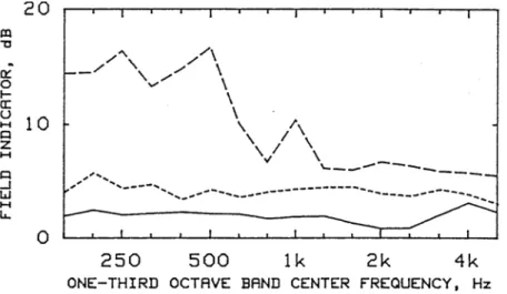
(3.17) is the global pressure-intensity index of the measurement. Comparing eqs. (3.7) and (3.15) shows that this quantity plays the same rôle in sound power estimation as the pressure-intensity index does in measurements at discrete points. Figure 3.4 shows examples of the global index measured under various conditions. It is obvious that the presence of noise sources outside the measurement surface increases the mean square pressure on the surface, and thus the influence of a given phase error; therefore a phase error, no matter how small, limits the range of measurement.
In practice one should examine whether the inequality (3.16) is satisfied or not whenever there is significant noise from extraneous sources. If the inequality is not satisfied it can be recommended to use a measurement surface somewhat closer to the source than advisable in
more favourable circumstances. It may also be necessary to modify the measurement conditions – to shield the measurement surface from strong extraneous sources, for example, or to increase the sound absorption in the room. All modern sound intensity analysers can determine the pressure-intensity index concurrently with the actual measurement, so one can easily check whether phase mismatch is a problem or not. Some instruments automatically examine whether the condition (3.16) (or (3.12) in a point measurement) is satisfied or not and give warnings when this is not the case.
Figure 3.4 The global pressure-intensity index )pI determined under three different conditions. ))) , Measurement
using a ‘reasonable’ surface; - - -, measurement using an eccentric surface; )) )), measurement with strong background noise. (From reference [34].)
Random errors associated with a given finite averaging time
Random errors due to incomplete time averaging reveal themselves by poor repeatability. Such errors can be of concern in several applications of sound intensity measure-ments. The averaging time needed to ensure a given accuracy depends very much of the local properties of the sound field, and some positions will require a very long averaging time. This is not very important if the sound intensity is averaged over a measurement surface, since the random errors are largest at positions that do not contribute much to the surface integral [35]. However, it is obviously inconvenient to use a very long averaging time at each point if the sound intensity is to be mapped in front of a large, complicated source of noise. In fact, even if an automated measurement system is available, the averaging time may be of concern, for example because the sound source under study is not completely stable over a long period of time.
That the normalised random errors in sound intensity measurements can be much larger than the theoretical minimum value of known from mean square estimation, where B is the bandwidth and T is the averaging time, was pointed out as early as in 1975 [36]. Some years later theoretical expressions were derived that showed that the random errors can be very large when the phase angle between two pressure signals from the sound intensity probe is small and the coherence of the signals is less than unity [27, 28].
It can be shown that the above mentioned additional random error due electrical noise in the microphone signals can be written [29]
where nrms is the rms value of the noise signals that contaminate the microphone signals and )N
is the phase angle between the two pressure signals, cf. eq. (2.22). The right-hand side of the equation shows that this error is inversely proportional to the signal-to-noise ratio and inversely proportional to the phase angle between the two sound pressure signals, which can be very small indeed; therefore, an averaging time of several minutes can be required even with a fairly large signal-to-noise ratio. However, this is a problem only at low frequencies (say, below 100 Hz) and at fairly low sound pressure levels, say, less than 40 dB re 1 :Pa.
3.3 Testing and verification
By now it should be apparent that even a sound intensity probe of the highest quality will give erroneous results under sufficiently difficult sound field conditions. A standardised verification procedure therefore prescribes that the intensity probe should be exposed to the sound field in a standing wave tube with a specified standing wave ratio; when the sound intensity probe is drawn through this interference field the sound intensity indicated by the measurement system should be within a certain tolerance.
Figure 3.5 (a) Sound pressure level ( ))) ), particle velocity level ( )) )) ) and sound intensity level ( )) A )) ) in a standing wave field with a standing wave ratio of 24 dB. (b) Estimation error of a sound intensity measurement system with a residual pressure-intensity index of 14 dB (positive and negative phase error). (From reference [37].)
The sound pressure in a one-dimensional interference field is
(3.19) where R is the reflection factor at the termination (see, eg, ref. [4]). The corresponding amplitude is
(3.20) (see figure 3.5). The particle velocity is [4]
(3.21) and the corresponding amplitude is
(3.22) The sound intensity in this interference field follows from eq. (2.18):
(3.23) Figure 3.5 (a) illustrates how the sound pressure, the particle velocity and the sound intensity vary with position in a one-dimensional interference field with a standing wave ratio of 24 dB. It is apparent that the pressure-intensity index varies strongly with the position in such a sound field. Accordingly, the influence of a given phase error depends on the position. Figure 3.5 (b) shows how the sound intensity measured with a certain instrument will deviate from the true value as a function of the position in a standing wave tube with a standing wave ratio of 24 dB, which is the sound field specified in the IEC standard on sound intensity measurement systems. According to this IEC standard deviations within an interval of ± 1.5 dB are acceptable for ‘class 1 instruments’.
4. APPLICATIONS
Some of the most common practical applications of sound intensity measurements are now discussed briefly.
Sound power determination
One of the most important applications of sound intensity measurements is the determination of the sound power of operating machinery in situ. Sound power determination using intensity measurements is based on eq. (2.16), which shows that the sound power of a source is given by the integral of the normal component of the intensity over a surface that encloses the source, also in the presence of other sources outside the measurement surface. Neither an anechoic or a reverberation room is required. The analysis of errors and limitations presented in section 3.2 leads to the conclusion that the sound intensity method is suitable • for stationary sources in stationary background noise provided that
The method is not suitable
• for sources that operate in long cycles (because the sound field will change during the measurement)
• in non-stationary background noise (for the same reason)
• for weak sources of low frequency noise (because of large random errors caused by electrical noise in the microphone signals).
The surface integral can be approximated either by sampling at discrete points or by scanning manually or with a robot over the surface. With the scanning approach, the intensity probe is moved continuously over the measurement surface in such a way that the axis of the probe is always perpendicular to the measurement surface. The scanning procedure, which was introduced in the late 1970s on a purely empirical basis, was regarded with much scepticism for
more than a decade [38], but is now generally considered to be more accurate and far more convenient than the procedure based on fixed points [39]. A moderate scanning rate, say 0.5 ms-1,
and a ‘reasonable’ scan line density should be used, say 5 cm between adjacent lines if the surface is very close to the source, 20 cm if it is further away. One cannot use the scanning method if the source is operating in cycles, though; both the source under test and possible extraneous noise sources must be perfectly stationary.
Usually the measurement surface is divided into a number of segments, each of which will be convenient to scan. One will often determine the pressure-intensity index of each segment, and the accuracy of each partial sound power estimate will of course depend on whether the inequality (3.16) is satisfied or not, but it follows from eq. (3.15) that it is the global pressure-intensity index associated with the entire measurement surface that determines the accuracy of the estimate of the (total) radiated sound power. It may be impossible to satisfy (3.16) on a certain segment, for example because the net sound power passing through the segment takes a very small value because of extraneous noise, but if the global criterion is satisfied then the total sound power estimate will nevertheless be accurate.
Theoretical considerations seem to indicate the existence of an optimum measurement surface that minimises measurement errors. In practice one uses a surface of a simple shape at some distance, say 25-50 cm, from the source. If there is a strong reverberant field or significant ambient noise from other sources, the measurement surface should be chosen to be somewhat closer to the source under study.
Noise source identification and visualisation of sound fields
This is another important application of the sound intensity method. A noise reduction project usually starts with the identification and ranking of noise sources and transmission paths, and sound intensity measurements make it possible to determine the partial sound power contribution of the various components directly. Two-dimensional contour plots of the sound intensity normal to a measurement surface can be used in locating noise sources. Visualisation of sound fields, helped by modern computer graphics, contributes to our understanding of radiation and propagation of sound and of diffraction and interference effects. However, since measurements at many discrete points are needed random errors associated with the finite averaging time can be a problem, in particular at positions where the sound radiation is weak. Transmission loss of structures and partitions
The conventional measure of the sound insulation of panels and partitions is the transmission loss (also called sound reduction index), which is the ratio of incident to transmitted sound power in logarithmic form. The traditional method of measuring this quantity requires a transmission suite consisting of two vibration-isolated reverberation rooms. The sound power incident on the partition under test in the source room is deduced from an estimate of the spatial average of the mean square sound pressure in the room on the assumption that the sound field is diffuse, and the transmitted sound power is determined from a similar measurement in the receiving room where, in addition, the reverberation time must be determined. The sound intensity method has made it possible to measure the transmitted sound power directly using a sound intensity probe. In this case it is not necessary that the sound field in the receiving room is diffuse, which means that only one reverberation room (the source room) is necessary [40]. One cannot measure the incident sound power in the source room using sound intensity, since the method gives the net sound intensity.
The main advantage of the intensity method over the conventional approach is that it is possible to evaluate the transmission loss of individual parts of the partition. However, each sound power measurement must obviously satisfy the condition
There are other sources of error than phase mismatch. For example, Roland has called attention to the fact that the traditional method of measuring the sound power transmitted through the partition under test gives the transmitted sound power irrespective of the absorption of the partition, whereas the intensity method gives the net power [41]. If a significant part of the absorption in the receiving room is due to the partition then the net power is less than transmitted power. Under such conditions one must increase the absorption of the receiving room; otherwise the intensity method will overestimate the transmission loss because the transmitted sound power is underestimated.
It has often been reported that the intensity method gives lower values of the transmission loss than the conventional one at low frequencies and higher values at high frequencies. However, this pattern has not been confirmed by a recent investigation in which very good agreement was found from 80 Hz to 6.3 kHz [42].
As an interesting byproduct of the intensity method it can be mentioned that deviations observed between results determined using the traditional pressure-based method and the intensity method led several authors to re-analyse the traditional method in the 1980s [43, 44] and point out that the Waterhouse correction [45], well established in sound power determination using the reverberation room method, had been overlooked in the standards for conventional measurements of transmission loss (the ISO 140 series). For more than a decade various authors expressed different opinions about whether the Waterhouse correction should be applied in the source room and not just in the receiving room; see, e.g., [46]. Much later a correction for the extra incident sound power in the source room was derived and it was shown that from a practical point of view it will be cancelled by the Waterhouse correction on the receiving side; in other words that no correction should be applied in conventional pressure-based measurements [47]. However, this cancellation occurs only if the partition is a complete wall [47].
Measurement of the emission sound pressure level
The ‘emission sound pressure level’ is the sound pressure level at an operator’s position near a large machine. There is now a standard based on the idea of deducing this level from sound intensity measurements in order to reduce the influence of certain sources of error.
Measurement of absorption
In principle it should be possible to measure the sound absorption of materials in situ using sound intensity, but so far this has generally been regarded as the least successful application of the method. Recent results have indicated that it may be possible to do it, though, but more work is needed.
REFERENCES
1. P.M. Morse and K.U. Ingard: Theoretical Acoustics. McGraw-Hill, New York, 1968. 2. A.D. Pierce: Acoustics: An Introduction to Its Physical Principles and Applications. 2nd
edition, Acoustical Society of America, New York, 1989.
3. S.W. Rienstra and A. Hirchberg: An introduction to acoustics. Report 1WDE99-02, Instituut Wiskundige Dienstverlering Eindhoven, Technische Universiteit Eindhoven, The Netherlands, 1999.
4. F. Jacobsen: Propagation of sound waves in ducts. Acoustic Technology, Department of Electrical Engineering, Technical University of Denmark, note no 31260, 2010. 5. F. Jacobsen and P.M. Juhl: Radiation of sound. Acoustic Technology, Department of
Electrical Engineering, Technical University of Denmark, 2010.
6. J.A. Mann III, J. Tichy and A.J. Romano: Instantaneous and time-averaged energy transfer in acoustic fields. Journal of the Acoustical Society of America 82, 17-30, 1987. 7. J.-C. Pascal: Mesure de l’intensité active and réactive dans different champs acoustiques. Proceedings of International Congress on Recent Developments in Acoustic Intensity Measurement, Senlis, France, 1981, pp. 11-19.
8. F. Jacobsen: Active and reactive, coherent and incoherent sound fields. Journal of Sound and Vibration 130, 493-507, 1989.
9. P.J. Westervelt: Acoustical impedance in terms of energy functions. Journal of the Acoustical Society of America 23, 347-349, 1951.
10. W. Maysenhölder: The reactive intensity of general time-harmonic structure-borne sound fields. Proceedings of Fourth International Congress on Intensity Techniques, Senlis, France, 1993, pp. 63-70.
11. F. Jacobsen, A note on instantaneous and time-averaged active and reactive sound intensity. Journal of Sound and Vibration 147, 489-496, 1991.
12. W.F. Druyvesteyn and H.E. de Bree: A novel sound intensity probe. Comparison with the pair of pressure microphones intensity probes. Journal of the Audio Engineering Society 48, 49-56, 2000.
13. R. Raangs, W.F. Druyvesteyn and H.-E. de Bree: A low-cost intensity probe. Journal of the Audio Engineering Society 51, 344-357, 2003.
14. F. Jacobsen and H.-E. De Bree: A comparison of two different sound intensity measurement principles. Journal of the Acoustical Society of America 118, 1510-1517, 2005.
15. F. Jacobsen and V. Jaud: A note on the calibration of pressure-velocity sound intensity probes. Journal of the Acoustical Society of America 120, 830-837, 2006.
16. F.J. Fahy: Measurement of acoustic intensity using the cross-spectral density of two
microphone signals. Journal of the Acoustical Society of America 62, 1057-1059, 1977. 17. J.Y. Chung: Cross-spectral method of measuring acoustic intensity without error caused by instrument phase mismatch. Journal of the Acoustical Society of America 64, 1613-1616, 1978.
18. F. Jacobsen, V. Cutanda and P.M. Juhl: A numerical and experimental investigation of the performance of sound intensity probes at high frequencies. Journal of the Acoustical Society of America 103, 953-961, 1998.
19. J. Pope: Qualifying intensity measurements for sound power determination. Proceedings of Inter-Noise 89, Newport Beach, CA, USA, pp. 1041-1046, 1989.
20. U.S. Shirahatti and M.J. Crocker: Two-microphone finite difference approximation errors in the interference fields of point dipole sources. Journal of the Acoustical Society of America 92, 258-267, 1992.
21. G. Krishnappa: Interference effects in the two-microphone technique of acoustic intensity measurements. Noise Control Engineering Journal 21, 126-135, 1983. 22. F. Jacobsen: A simple and effective correction for phase mismatch in intensity probes.
Applied Acoustics 33, 165-180, 1991.
23. M. Ren and F. Jacobsen: Phase mismatch errors and related indicators in sound intensity measurement. Journal of Sound and Vibration 149, 341-347, 1991.
24. D.H. Munro and K.U. Ingard: On acoustic intensity measurements in the presence of mean flow. Journal of the Acoustical Society of America 65, 1402-1406, 1979. 25. F. Jacobsen: Intensity measurements in the presence of moderate airflow. Proceedings
of Inter-Noise 94, Yokohama, Japan, pp. 1737-1742, 1994.
26. F. Jacobsen: A note on measurement of sound intensity with windscreened probes. Applied Acoustics 42, 41-53, 1994.
27. A.F. Seybert: Statistical errors in acoustic intensity measurements. Journal of Sound and Vibration 75, 519-526, 1981.
28. F. Jacobsen: Random errors in sound intensity estimation. Journal of Sound and Vibration 128, 247-257, 1989.
29. F. Jacobsen: Sound intensity measurement at low levels. Journal of Sound and Vibration 166, 195-207, 1993.
30. E. Frederiksen and O. Schultz: Pressure microphones for intensity measurements with significantly improved phase properties. Brüel & Kjær Technical Review 4, 11-23, 1986. 31. F. Jacobsen and E.S. Olsen: The influence of microphone vents on the performance of
sound intensity probes. Applied Acoustics 41, 25-45, 1994.
32. S. Gade, Sound intensity (Theory). Brüel & Kjær Technical Review 3, 3-39, 1982. 33. S. Gade, Validity of intensity measurements in partially diffuse sound field. Brüel &
Kjær Technical Review 4, 3-31, 1985.
34. F. Jacobsen, Sound field indicators: Useful tools. Noise Control Engineering Journal 35, 37-46, 1990.
35. F. Jacobsen: Random errors in sound power determination based on intensity measurement. Journal of Sound and Vibration 131, 475-487, 1989.
36. B.G. van Zyl and F. Anderson: Evaluation of the intensity method of sound power determination. Journal of the Acoustical Society of America 57, 682-686, 1975. 37. F. Jacobsen and E.S. Olsen: Testing sound intensity probes in interference fields.
Acustica 80, 115-126, 1994.
38. M.J. Crocker: Sound power determination from sound intensity – To scan or not to scan. Noise Control Engineering Journal 27, 67, 1986.
39. U.S. Shirahatti and M.J. Crocker: Studies of the sound power estimation of a noise source using the two-microphone sound intensity technique. Acustica 80, 378-387, 1994.
40. M.J. Crocker, P.K. Raju and B. Forssen, Measurement of transmission loss of panels by the direct determination of transmitted acoustic intensity. Noise Control Engineering Journal 17, 6-11, 1981.
41. J. Roland and C. Martin and M. Villot: Room to room transmission: What is really measured by intensity? Proceedings of 2nd International Congress on Acoustic Intensity,
Senlis, France, pp. 539-546, 1985.
42. M. Machimbarrena and F. Jacobsen: Is there a systematic disagreement between intensity-based and pressure-based sound transmission loss measurements? Journal of Building Acoustics 6, 101-111, 1999.
43. R.E. Halliwell and A.C.C. Warnock: Sound transmission loss: Comparison of conventional techniques with sound intensity techniques. Journal of the Acoustical Society of America 77, 2094-2103, 1985.
44. B.G. van Zyl, P.J. Erasmus and F. Anderson: On the formulation of the sound intensity method for determining sound reduction indices. Applied Acoustics 22, 213-228, 1987.
45. R.V. Waterhouse: Interference patters in reverberant sound fields. Journal of the Acoustical Society of America 27, 247-258, 1955.
46. M. Vorländer: Revised relation between the sound power and the average sound pressure level in rooms and consequences for acoustic measurements. Acustica 81, 332-343 (1995).
47. F. Jacobsen and E. Tiana-Roig: Measurement of the sound power incident on the walls of a reverberation room with near field acoustic holography. Acta Acustica united with Acustica 96, 76-91 (2010).
BIBLIOGRAPHY
Frank Fahy’s monograph Sound Intensity summarises the wide range of publications on this topic up to 1995, and deals with practically all aspects of sound intensity and its measure1ment. The special issue of Applied Acoustics concentrates on sound power determina-tion based on sound intensity. The chapter in Handbook of Acoustics gives an introductory updated overview of the topic, whereas the chapter in Handbook of Signal Processing in Acoustics is concerned with the pressure-velocity sound intensity probe produced by Microflown. 1. F.J. Fahy: Sound Intensity. 2nd edition, E&FN Spon, London, 1995.
2. F. Jacobsen (ed.) Applied Acoustics 50 (2), 1997. Special issue on sound intensity measurement.
3. F. Jacobsen: Sound Intensity. Chapter 25 in Springer Handbook of Acoustics, ed. Thomas Rossing. Springer Verlag, New York, 2007.
4. F. Jacobsen and H.-E. de Bree: The Microflown particle velocity sensor. Chapter 68 (pp. 1283-1291) in Handbook of Signal Processing in Acoustics, eds. D. Havelock, S. Kuwano and M. Vorländer (Springer Verlag, New York, 2008).
LIST OF SYMBOLS B bandwidth [Hz] c speed of sound [m/s] E sound energy [J] f frequency [Hz] I sound intensity [W/m2]
Ir component of sound intensity [W/m2]
finite difference estimate of sound intensity component [W/m2]
Iref reference sound intensity [W/m2]
Io residual intensity [W/m2]
J reactive sound intensity [W/m2]
k wavenumber [m-1]
K bias error factor [dB] Ld dynamic capability [dB]
LI sound intensity level [dB re Iref]
Lp sound pressure level [dB re pref] p sound pressure [Pa]
sound pressure (complex representation) [Pa] finite difference estimate of sound pressure [Pa] pref reference sound pressure [Pa]
prms rms sound pressure [Pa] p0 static pressure [Pa]
po sound pressure used in determining the residual intensity [Pa]
Pa sound power [W]
Q volume velocity of source [m3/s]
r radial distance in cylindrical and spherical coordinate system [m] R gas constant [m2s-2K-1]; reflection factor [dimensionless]
S area [m2]
S12 cross spectrum of microphone signals [Pa2/Hz]
t time [s]
T averaging time [s] u particle velocity [m/s]
component of the particle velocity [m/s]
particle velocity (complex representation) [m/s]
finite difference estimate of particle velocity component [m/s] V volume [m3]
w total energy density [J/m3]
wpot potential energy density [J/m3]
wkin kinetic energy density [J/m3]
Zs specific impedance [kgm-2s-1]
( ratio of specific heats [dimensionless]
*pI pressure-intensity index [dB]
*pIo residual pressure-intensity index [dB] )pI global pressure-intensity index [dB]
)r microphone separation distance [m]
2 phase angle of reflection factor [radian]
n phase angle between sound pressure and particle velocity [radian]
N phase angle of complex pressure [radian]
ne phase error [radian]
T angular frequency [radian/s] ^ a finite difference estimate
~ complex representation of a harmonic variable G time averaging
APPENDIX A: COMPLEX NOTATION
In a harmonic sound field the sound pressure is a function of the type cos(Tt + n) at any point. It is common practice to use complex notation in such cases. This is a symbolic method that makes use of the fact that complex exponentials give a more condensed notation that trigonometric functions because of the complicated multiplication theorems of the latter.
Complex representation of harmonic signals is based on Euler’s equation,
(A1) In a harmonic sound field the sound pressure can be written
(A2) where A is the complex amplitude of the sound pressure. The real, physical sound pressure is of course a real function of the time,
(A3) which is seen to be an expression of the form cos(Tt + n). The magnitude of the complex quan-tity *A* is called the amplitude of the pressure, and nA is its phase, and these two quantities
depend on the position in the sound field.
Acoustic second-order quantities involve time averages of squared harmonic signals and, more generally, products of harmonic signals. Such quantities are dealt with in a special way, as follows. Expressed in terms of the complex pressure amplitude the mean square pressure becomes
(A4) in agreement with the fact that the average value of a squared cosine is ½. Note that it is the squared magnitude of that enters into the expression, not the square of which is a complex number proportional to e2jTt.
The time average of a product of harmonic signals is expressed as follows,
(A5)
(A6) Note that either or must be conjugated.
5For sound in other fluids than atmospheric air the reference sound pressure is 1 :Pa.
APPENDIX B: LEVELS AND DECIBELS
The human auditory system can cope with sound pressure variations over a range of more than a million times. Because of this wide range, the sound pressure and other acoustic quantities are usually measured on a logarithmic scale. An additional reason is that the subjective impression of how loud noise sounds correlates much better with a logarithmic measure of the sound pressure than with the sound pressure itself. The unit is the decibel, abbreviated dB, which is a relative measure, requiring a reference quantity. The results are called levels. The sound pressure level is defined as
(B1)
where pref is the reference sound pressure, and log10 is the logarithm to the base of 10, henceforth
written log. The reference sound pressure is 20 :Pa for sound waves in air,5 corresponding
roughly to the lowest audible sound at 1000 Hz.
The acoustic second-order quantities sound intensity and sound power are also measured on a logarithmic scale. The sound intensity level is
(B2)
where I is the intensity and Iref = 1 pWm-2 = 10-12 Wm-2, and the sound power level is
(B3) where Pa is the sound power and Pref = 1 pW. Note than levels of linear quantities are defined as twenty times the logarithm of the ratio of the rms value to a reference value, whereas levels of second-order quantities are defined as ten times the logarithm, in agreement with the quadratic relation between second-order and first-order quantities.
The simple relationship between the sound intensity and sound pressure in a plane propagating wave and in a simple spherical sound field,
(B4) implies that the sound intensity level is approximately equal to the sound pressure level in air under normal ambient conditions. This is due to the fact that the quantity is close to unity (or that is close to 400 kgm-2s-1). With the relations
and (B5a, B5b) where p0 is the static pressure, ( is the ratio of specific heats, R is the gas constant and T is the absolute temperature, it follows that
(B6)
which is close to unity under normal ambient conditions; it equals 1.028 at 101.325 kPa and 296.15 K = 23/C. This factor corresponds to 0.12 dB, which is a small correction. Accordingly,
For the same reason the pressure-intensity index
(B7) is sometimes written simply as Lp - LI.
APPENDIX C: STANDARDS FOR SOUND INTENSITY MEASUREMENTS
There are several international and national standards for the measurement of sound intensity:
ISO (International Organization for Standardization) 9614-1 Acoustics ) Determination of Sound Power Levels of Noise Sources Using Sound Intensity ) Part 1: Measurement at Discrete Points, 1993.
ISO (International Organization for Standardization) 9614-2 Acoustics ) Determination of Sound Power Levels of Noise Sources Using Sound Intensity ) Part 2: Measurement by Scanning, 1996.
ISO (International Organization for Standardization) 9614-3 Acoustics ) Determination of Sound Power Levels of Noise Sources Using Sound Intensity ) Part 3: Precision Method for Measurement by Scanning, 2002.
IEC (International Electrotechnical Commission) 1043 Electroacoustics ) Instruments for the Measurement of Sound Intensity ) Measurements with Pairs of Pressure Sensing Microphones, 1993.
ANSI (American National Standards Institute) S12.12-1992 Engineering Method for the Determination of Sound Power Levels of Noise Sources Using Sound Intensity.
ANSI (American National Standards Institute) S1.9-1996 Instruments for the Measurement of Sound Intensity.
ISO (International Organization for Standardization) 15186-1 Acoustics ) Measurement of Sound Insulation in Buildings and of Building Elements ) Part 1: Laborary measurements, 2000. ISO (International Organization for Standardization) 15186-2 Acoustics ) Measurement of Sound Insulation in Buildings and of Building Elements ) Part 2: Field measurements, 2003. ISO (International Organization for Standardization) 11205 Acoustics ) Determination of Emission Sound Pressure Levels In Situ at the Work Station and other Specified Positions Using Sound Intensity, 2003.
INDEX
Absorption, measurement of, 26 Acoustic energy
see Sound energy Acoustic intensity
see Sound intensity Active sound field, 11
see also Reactive sound field Adiabatic compressibility, 6
Airflow, influence of, 17 Amplitude gradient, 13 Averaging time, 22 Bias errors, 17 Bias error factor, 21 Complex notation, 33 Complex sound intensity, 14 Conservation of mass, 6 Conservation of momentum, 7 Conservation of sound energy, 7 Diffraction, 19
Diffuse sound field, 13
Discrete points, measurements at, 25 Dynamic capability, 21
Electrical noise, effect of, 23 Emission sound pressure level, 26 Energy acoustics, 5
Euler’s equation of motion, 7 Face-to-face arrangement, 17 Far field approximation, 10
Finite difference approximation, 18 Free-field method, 10
Frequency domain formulation, 16 Frequency range of measurement, 19 Gauss’s theorem, 7
Global pressure-intensity index, 21 Hot wire anemometer, 15
Identification of sources, 25 Incoherent sources
see Uncorrelated sources In-phase component, 10
Instantaneous energy density, 7
Instantaneous sound intensity, 6 Interference field, 23
Impedance
characteristic, 9, 35 radiation, 11 specific, 11 Kinetic energy density, 6 Linearised acoustic equations, 7 Location of sources, 25
Measurement standards, 37 Measurement surface, 25
Microphone separation distance, 18 Nearfield characteristics, 11 Particle velocity, 6 Phase error, 19 Phase mismatch, 19 Phase gradient, 10 Plane wave, 9, 19
Potential energy density, 6 p-p measurement principle, 15 Pressure-intensity index, 20, 36 p-u measurement principle, 15 Quadrature, 13
Random errors, 17, 22 Rank order of sources, 25 Reactive sound field, 13 Reactive sound intensity, 11 Reference value, 35
Residual intensity, 20
Residual pressure-intensity index, 20 Scanning method, 25
Scattering
see Diffraction Simple spherical field, 9, 10 Sound energy, 6
Sound intensity, 7
Sound power determination, 8, 24 Spacer, 17, 19
Standing wave tube, 23 Surface segments, 25 Superposition, 8
Testing and verification, 23
Time averaged sound intensity, 7, 10 Time domain formulation, 16
Transmission loss, 25 Two-microphone method
see p-p measurement principle Uncorrelated sources, 8
Visualisation of sound fields, 25 Waterhouse correction, 26 Weak sources, 23, 25 Windscreens, 17
![Figure 2.1 Measurement in an active sound field (from reference [11]). (a) )) , Instantaneous sound pressure; - - - , instantaneous particle velocity multiplied by D c](https://thumb-us.123doks.com/thumbv2/123dok_us/471444.2555671/12.892.245.640.355.824/measurement-reference-instantaneous-pressure-instantaneous-particle-velocity-multiplied.webp)
![Figure 2.2 Measurement in a reactive sound field (from reference [11]). Key as in figure 2.1](https://thumb-us.123doks.com/thumbv2/123dok_us/471444.2555671/13.892.223.655.102.668/figure-measurement-reactive-sound-field-reference-key-figure.webp)
![Figure 2.3 Measurement in a diffuse sound field (from reference [11]). Key as in figure 2.1](https://thumb-us.123doks.com/thumbv2/123dok_us/471444.2555671/14.892.240.648.313.814/figure-measurement-diffuse-sound-field-reference-key-figure.webp)