Comparison of Kernel Support Vector Machine (SVM) in Classification of Human Development Index (HDI)

(1)

Comparison of Kernel Support Vector Machine

(SVM) in Classification of Human

Development Index (HDI)

Harun Al Azies1_{, Dea Trishnanti}2_{, Elvira Mustikawati P.H}3

Abstract Human Development Index (HDI) is one of measuring instrument of achieving quality of life of one region even country. There are three basic components of the Human Development Index compilers: health dimension, knowledge dimension, and decent living dimension. Classification is a method for compiling data systematically according to the rules that have been set previously. In recent years, classification method has been proven to help many people’s work, such as image classification, medical biology, traffic light, text classification etc. There are many methods to solve classification problem. This variation method makes the researchers find it difficult to determine which method is best for a problem this framework is aimed to compare the ability of classification methods, such as Support Vector Machine (SVM) Linear Kernel, Radial Basis Function (RBF) Kernel and Polynomial kernel methods. The result of classification of HDI by using RBF kernel is the best kernel to solve HDI problem, with parameter combination cost= 1 and gamma=1 obtained classification accuracy of 98.1% which is the best classification accuracy.

KeywordsClassification, HDI, Support Vector Machine, Linear Kernel, RBF Kernel, Polynomial kernel.

I. INTRODUCTION

The human development index is one measure of achieving the quality of life of an area or country. There are 3 basic components of the Human Development Index (HDI), namely the health dimension, the knowledge dimension, and the decent living dimension [1]. To measure the dimensions of health, life expectancy at birth is used. Next to measure the dimensions of knowledge used a combination of indicators of school long expectations and the average length of school. The decent living dimension is used as an indicator of people's purchasing power to a number of basic needs as seen from the average amount of expenditure per capita adjusted. [1]. Indonesia is a developing country where every district and city in the province has a wide HDI value. Human Development Index (HDI) according to the Central Statistics Agency [1] is divided into 4 categories or groups namely Human Development Index _______________________

1_{Department of Statistics, PGRI Adi Buana University, Surabaya,} 60234, Indonesia. E-mail:harunalazies@gmail.com

2_{Department of Statistics, PGRI Adi Buana University, Surabaya,} 60234, Indonesia. E-mail: trishnantidea@gmail.com

3_{Department of Statistics, PGRI Adi Buana University, Surabaya,} 60234, Indonesia. E-mail: elvira@unipasby.ac.id

(HDI) low (<60), moderate (60 ≤ HDI <70), high (70 ≤ HDI <80), and very high (≥ 80) [1]. Because development in Indonesia is uneven, the HDI in regions, especially districts / cities, is very diverse. HDI with high to very high categories is only found in regencies/big cities in Indonesia, because in regencies/big cities in Indonesia have adequate health, education and needs facilities. In contrast to areas outside of Java that tend to have uneven distribution of HDI.

Data mining works to gather information from a large amount of data. Jobs closely related to data mining are prediction modeling, cluster analysis, association analysis, and anomaly detection [2]. The methods contained in data mining include Artificial Neural Network (ANN), Support Vector Machine (SVM), k-Nearset Neighbor (k-NN) and Naïve Bayes.

Support Vector Machine (SVM) is a classification method introduced by Vapnik in 1995[3]. Support Vector Machine (SVM) belongs to the Artifical Neural Network (ANN) class. In classifying the Support Vector Machine (SVM) there is a need for training stages and testing stages. The advantage of Support Vector Machine (SVM) compared to Artificial Neural Network (ANN) is in terms of the solution achieved, where Artifical Neural Network (ANN) solution is obtained in the form of optimal local, while Support Vector Machine (SVM) is optimal global. The goal of the Support Vector Machine (SVM) method is to find an optimal classifier function that can separate two different data sets [3]. The best separator or hyperplane function is the hyperplane that is caught in the middle of two objects from both classes.

This study uses a cross-sectional study to explain the relationship between the independent variable or risk factor and the dependent variable. The dependent variable is a binary data or dichotomous. In the previous research, the study comparison of kernel function such as RBF, linear and polynomial has been conducted and as a result showed that the RBF kernel function has the highest performance for text or image document categorization [4].

The Support Vector Machine (SVM) is a type of machine learning, based on statistical learning theory, which contains polynomial classifiers, neural networks, and radial basis function (RBF) networks as special cases. In the RBF case, the SV algorithm automatically determines centers, weights, and threshold that minimize an upper bound on the expected test error. Therefore, this research is purposed to investigate the classification of

(2)

the Human Development Index (HDI) performance between Linear Kernel, RBF Kernel and Polynomial kernel

II. METHOD

A. Support Vector Machine (SVM)

Support Vector Machine (SVM) is included in the Artifical Neural Network (ANN) class. In classifying the Support Vector Machine (SVM) there is a need for training stages and testing stages. The goal of the Support Vector Machine (SVM) method is to find an optimal classifier function that can separate two different data sets [3]. The best separator or hyperplane function is the hyperplane that is caught in the middle of two objects from both classes. The linear function of SVM:

( )

x sign

(

f

( )

x

)

g = (1) With

( )

x w x b f = T + (2)

𝑥, 𝑤 𝜖𝑅𝑛_and_𝑏𝜖𝑅_{this classification problem can be} formulated as below: to find the value of a parameter (𝑤,

𝑏) then 𝑠𝑔𝑛(𝑓(𝑥𝑖)) = 𝑠i𝑔𝑛(< 𝑤, 𝑥 > +𝑏) = 𝑦𝑖 for i.

If the set 𝑋 = {𝑥1, 𝑥2, …, 𝑥𝑛}, expressed as a positive

class if 𝑓(𝑥) ≥ 0 and others are included in the negative. SVM classifies the training vector set in the form of paired data sets from two classes [3] is (𝑥𝑖,𝑦𝑖),𝑥𝑖𝜖𝑅𝑛,𝑦𝑖 𝜖 {1,−1},𝑖=1,…,𝑛

Optimize hyperplane by enlarging 2‖𝑤‖ or minimize

𝜑(𝑤)= [8]. This optimization problem can be

solved by using the Lagrange function:

(3)

Which 𝛼𝑖 is the Lagrange function multiplier. The

equation is a primal space equation so it needs to be transformed into dual space.

(4)

with restrictions, ,

In the non-separable case some data might not be grouped correctly, then the objective function is modified by including the slack variable 𝜉 > 0. Then the equation becomes below [8].

(5)

with restrictions 𝑦𝑖 [(𝑤𝑇_𝑥𝑖_{) +}_𝑏_{] +}_𝜉𝑖_{≥ 1}_𝑖_{= 1,2, … ,}_𝑛 In the case of separable and non-sparable differences between the two lies in the addition of constraints 0 ≤ 𝛼𝑖

≤ 𝐶 on separable problems [5]. In the case of non-linear optimization the equation becomes below:

(6) With restrictions 0≤𝛼 ≤ 𝐶, 𝑖 = 1, … , 𝑛 and

𝐾(𝑥𝑖, 𝑥𝑗) is a kernel function used to handle non-linear data. obtained functions for non-linear as below:

₍₇₎

All value 𝑓(𝑥) < 0 labeled " − 1" and 𝑓(𝑥) > 0 labeled " + 1". Various types of kernels.

Linier j T i j i K(x ,x )=x x (8) Polynomial d j T i j i K(x ,x )=(x x +1) (9)

Gaussian/Radial Basis Function (RBF)

d j T i j i K(x ,x )=(x x +1) (10)

B. Data Sources and Research Variables

This study uses a cross-sectional study to explain the relationship between independent variables or risk factors and the dependent variable. The data used in this study are secondary data obtained from the official publication of the Central Statistics Agency [1] on the Human Development Index, Life Expectancy, Average Length of Schooling, Expectancy of Old School, and expenditure per capita adjusted in 2018 with a total of 541 data namely data for each district / city in Indonesia [1]. With the data structure found in Table 1.

TABLE 1. RESEARCH VARIABLES

Variable Category Scale

Human Development Index (Y)

1 = Low HDI

Ordina l 2 = Medium HDI 3 = High HDI 4 = Very High HDI [11]

Life Expectancy (X1) - Ratio

Expected Years of Schooling

(X2) - Ratio

Mean Years of Schooling (X3) - Ratio Per capita expenditure (X4) - Ratio The dataset was divided into 2 parts, training data (80%) and testing data (20%) as in Table 2.

(3)

TABLE 2. CLASSIFICATION DATASET

Amount Data Set Training Data Set Testing Data Set

514 411 103

Taking training dataset and testing the dataset is done randomly with the help of python software. As explained in the research method in the previous chapter, classification methods will be used contained in data mining namely Support Vector Machine (SVM) to find the best accuracy value.

III. RESULTS AND DISCUSSION

A. Overview of HDI in Indonesia

Figure 1. Descriptive Statistics of Overview of HDI in Indonesia Based on Figure 1 it can be seen that 57 percent or around 296 districts / cities in Indonesia have a moderate HDI which is an HDI value between 60 ≤ HDI <70. Meanwhile 32 percent or around 163 districts / cities in Indonesia have a high HDI that is a HDI value between 70 ≤ HDI <80. While 5 percent or around 26 regencies / cities in Indonesia have low HDI, that is, the HDI value is less than 60 with Nduga Regency in Papua Province is the region with the lowest HDI in Indonesia, amounting to 29.42. While the remaining 29 districts / cities in Indonesia have a very high HDI that is an HDI value of more than 80, Yogyakarta is the region in Indonesia with the highest HDI of 86.11

B. Support Vector Machine (SVM) Result

The analytical method that will be used in research is to use Support Vector Machine (SVM). In the use of the SVM method a separation of training dataset and testing dataset will be performed. The training dataset is taken 80% of the total of 514 sample data. As for testing the dataset is the remainder of the data to be tested for accuracy. Taking training dataset and testing the dataset is done randomly with the help of python software. The following is a visualization of the dataset used.

Figure 2 above explains that the data is divided into four groups, namely districts / cities that have low, medium, high to very high HDI. Therefore, one of the classification techniques that can be used is the Support Vector Machine (SVM) Method, As explained in the research method in the previous chapter, three SVM functions will be used to find the best accuracy value,

Figure 2. Distribution of Data Based on HDI Categories including linear SVM, SVM kernel RBF, and SVM kernel polynomial which will be discussed one by one as below

C. Linear Kernel SVM

Linear Kernel SVM is a good kernel function to use when the data is linearly separated. The analysis was performed using 869 samples divided into two parts, 80% as a training dataset and another 20% as a testing dataset. In analyzing the linear kernel function, the C or Cost parameters are optimized. Optimization of parameter C can be done by trial and error [10]. Here is a table determining the best linear kernel parameters by trial and error.

TABLE 3.

THE BEST PARAMETERS ACCURACY BY LINEAR KERNEL

Parameter Accurate

C = 0.0001 0.495

C = 0.001 0.495

C = 0.01 0.951

From the overall trial and error carried out, the same accuracy is obtained for each cost parameter so that the determination of the best parameters can be done by selecting one of the cost parameter values. The author will use C = 0.01 as the best parameter in forming the model by testing the dataset. So that the parameters of the model will be obtained are as below.

TABLE 4.

PARAMETERS OF THE LINEAR KERNEL

SVM-Type SVM-Kernel Cost

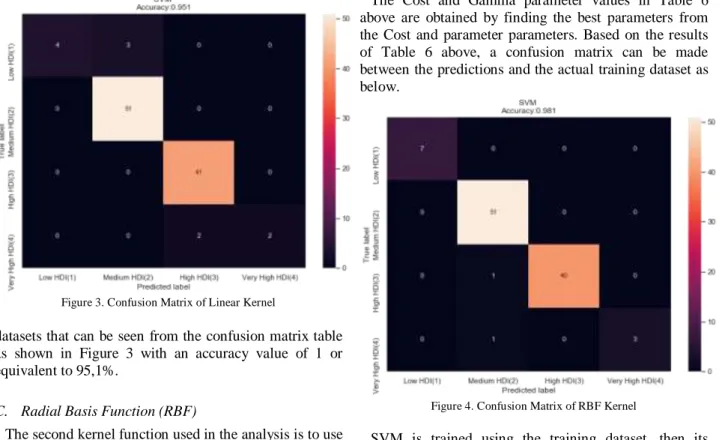
C – Classification Linear 0.01 Based on Table 4 above, when the linear kernel function is used in analyzing the results, the best parameter for C parameter is 0.01. From the results of obtaining the best parameters above, a confusion matrix can be made between the predictions and the actual testing dataset as below.

SVM is trained using the training dataset, then its performance is evaluated in the testing dataset. When an SVM analysis is performed using the Linear kernel function, the results show that SVM will correctly classify 98 samples from a total of 103 sample

(4)

testing

Figure 3. Confusion Matrix of Linear Kernel

datasets that can be seen from the confusion matrix table as shown in Figure 3 with an accuracy value of 1 or equivalent to 95,1%.

C. Radial Basis Function (RBF)

The second kernel function used in the analysis is to use the SVM kernel RBF as explained in the foundation theory chapter, the RBF kernel is a kernel function that is used when data is not linearly separated. In analyzing the kernel RBF function, the cost (C) and Gamma (γ) parameters are optimized. The analysis was performed using 869 samples divided into two parts, 80% as a training dataset and another 20% as a testing dataset. Just as in the linear kernel function, in determining the best parameters in the kernel RBF also carried out trial and error so the following table will be obtained

From the entire trial and error conducted, in Table 5 the results obtained are almost the same accuracy on each cost parameter and γ so that the determination of the best parameters can be done by selecting one of the cost parameters and γ.

TABLE 5.

THE BEST PARAMETERS ACCURACY BY RBFKERNEL

Parameter Accurate

γ = 1 γ =2 γ =3

C = 1 0.981 0.942 0.902

C = 2 0.981 0.942 0.913

C = 3 0.981 0.942 0.913

The researcher will use C = 1, and γ = 1 as the best parameter in forming the model by testing the dataset. So that the parameters of the model will be obtained are as below.

TABLE 6.

PARAMETERS OF THE RBFKERNEL

SVM-Type SVM-Kernel Cost Gamma

C – Classification Radial 1 1

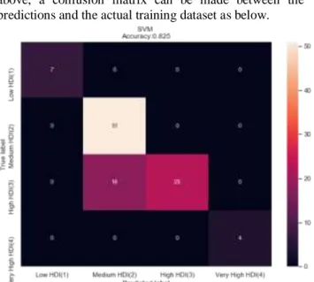
The Cost and Gamma parameter values in Table 6 above are obtained by finding the best parameters from the Cost and parameter parameters. Based on the results of Table 6 above, a confusion matrix can be made between the predictions and the actual training dataset as below.

Figure 4. Confusion Matrix of RBF Kernel

SVM is trained using the training dataset, then its performance is evaluated in the testing dataset. When an SVM analysis is performed using the RBF kernel function, the results show that SVM will classify 101 samples correctly from a total of 103 sample testing datasets that can be seen from the confusion matrix table as shown in Figure 4 with an accuracy value of 0.981 or equal to 98.1%.

D. Polynomial Kernel SVM

The third kernel function used in the analysis is to use the Polynomial kernel as explained in the foundation theory chapter, the Polynomial kernel is a kernel function that is used when data is not linearly separated. In analyzing the kernel RBF function, the cost (C) and degree value (d) parameters are optimized. The analysis was performed using 869 samples divided into two parts, 80% as a training dataset and another 20% as a testing dataset. Just as in the linear kernel function, in determining the best parameters in the Polynomial kernel also carried out trial and error so the following table will be obtained

TABLE 7.

THE BEST PARAMETERS ACCURACY BY POLYNOMIAL KERNEL

Parameter Accurate d = 4 d = 5 d = 6 C = 1 0.734 0.777 0.728 C = 2 0.777 0.816 0.738 C = 3 0.816 0.825 0.748

From the overall trial and error conducted, in Table 7 the accuracy of several parameters cost and d is obtained. The results in the table show that the accuracy at C = 3 with the degree value (d) = 5 is 0.825. The author will use

(5)

C = 3, and d = 5 as the best parameter in the formation of the model by testing the dataset. So that the parameters of the model will be obtained are as below.

TABLE 8.

PARAMETERS OF THE RBFKERNEL

SVM-Type SVM-Kernel Cost Degree

C – Classification Polynomial 3 5 The Cost and degree parameters (d) in Table 8 above are obtained by finding the best parameters of the Cost and degree parameters. Based on the results of Table 8 above, a confusion matrix can be made between the predictions and the actual training dataset as below.

Figure 5. Confusion Matrix of Polynomial Kernel

SVM is trained using the training dataset, then its performance is evaluated in the testing dataset. When an SVM analysis is performed using the polynomial kernel function, the results show that SVM will classify 85 correctly from a total of 103 sample testing datasets that can be seen from the confusion matrix table as shown in Figure 5 with an accuracy value of 0.825 or equal to 82.5%.

E. Comparison of the Three Functions of the SVM Kernel

After conducting the analysis using the linear kernel function, RBF, as well as the HDI polynomial districts and cities in Indonesia. Then it will be determined which kernel function is most suitable to be used in determining the accuracy of HDI classification of districts and cities in Indonesia. The following is a summary of the accuracy values of the three kernel functions.

Figure 6. Accuracy Comparison Chart based on Kernel Tricks used in SVM

Gamma and C parameter values are used as input for the classification process so as to produce an accuracy level, following the best accuracy level comparison based on gamma and C values for Support Vector Machine (SVM). Support Vector Machine (SVM) with 98% accuracy is a RBF kernel function with a combination of parameters C = 1. For data mining classification, the accuracy value can be divided into several groups [3].

0.90 - 1.00 = very good classification. 0.80 - 0.90 = good classification 0.70 - 0.80 = enough classification 0.60 - 0.70 = bad classification 0.50 - 0.60 = wrong classification

Based on the discussion above it can be concluded that the results of the classification of the Human Development Index (HDI) with the Radial Basis Function Support Vector Machine (SVM) methods are included in the very good classification level. The result of classification of HDI by using RBF SVM method is the best method to solve HDI problem, with parameter combination cost=1 and gamma=1 obtained classification accuracy of 98,1% which is the best classification accuracy

IV. REFERENCES

[1] Badan Pusat Statistik, Indeks Pembangunan Manusia 2018. Jakarta: Badan Pusat Statistik RI, 2018.

[2] Prasetyo E., Data Mining Konserp dan Aplikasi Menggunakan MATLAB. Yogyakarta: Andi, 2012.

[3] Vapnik, The Natural of Statistical Learning Thoery. New York: Springer, 1995.

[4] M. Yekkekhany, G., Safari, A., Homayouni, S., and Hasanlou, “A Comparison study of different kernel functions for SVM-based classification of multi-temporal polametry SAR data,” Volume XL-2W3, 2014.

[5] Novianti FA and Purnami SW, “Analisis Diagnosis Pasien Kanker Payudara Menggunakan Regresi Logistik dan Support Vector Machine (SVM) Berdasarkan Hasil Mamografi,” J. Sains dan Seni ITS, vol. 1, no. 1, 2012.