Variational Bayesian Algorithm For Distributed
Compressive Sensing
Wei Chen
∗†and Ian J. Wassell
†∗ State Key Laboratory of Rail Traffic Control and Safety, Beijing Jiaotong University, China † Computer Laboratory, University of Cambridge, UK
[email protected], [email protected]
Abstract—Distributed compressive sensing (DCS) concerns the reconstruction of multiple sensor signals with reduced numbers of measurements, which exploits both intra- and inter-signal correlations. In this paper, we propose a novel Bayesian DCS algorithm based on variational Bayesian inference. The proposed algorithm decouples the common component, that character-izes inter-signal correlation, from innovation components, that represent intra-signal correlation. Such an operation results in a computational complexity of reconstruction which is linear with the number of signals. The superior performance of the algorithm, in terms of the computing time and reconstruction quality, is demonstrated by numerical simulations in comparison with other existing reconstruction methods.
Index Terms—Distributed compressive sensing (DCS), Bayesian inference, signal reconstruction.
I. INTRODUCTION
C
OMPRESSIVE sensing (CS) [1], [2] enables one to reconstruct compressible signals from a reduced number of linear measurements. Owning to its convenience for data acquisition, CS has been proposed to take the place of the traditional sampling-and-compression approach in applications such as wireless sensor networks (WSNs) where data acquisi-tion is costly. In a WSN, the sensor nodes are embedded into the environment being sensed, which often places stringent constraints on power consumption, since it may be highly impractical to regularly replace or recharge embedded or implanted batteries, especially if there are many nodes forming a network. By applying CS, the number of samples required can be reduced and the compression operation is simpler than that for traditional compression methods. It has been shown that the limited energy supply in WSNs can be used more efficiently with CS, which leads to a longer network lifetime [3]–[5].CS exploits the sparse structure of a signal and applies random measurements. However, in WSN applications, dense-ly deployed sensors within the event area have high spatial correlations. Such spatial correlations, which represent inter-signal correlations, are not considered in conventional CS. To further exploit inter-signal correlations, the CS framework has This work is supported by EPSRC Research Grant (EP/K033700/1); the Natural Science Foundation of China (61401018, U1334202); the State Key Laboratory of Rail Traffic Control and Safety (RCS2014ZT08), Beijing Jiao-tong University; the Fundamental Research Funds for the Central Universities (2014JBM149); the Key Grant Project of Chinese Ministry of Education (313006); the Scientific Research Foundation for the Returned Overseas Chinese Scholars, State Education Ministry.
been extended for multiple measurement vectors (MMVs) [6], [7] which, similarly to sparse signal reconstruction, jointly recover a set of signals. The MMVs model assumes that all signals share a common support, which may not be true in WSN applications. In [8], [9], distributed compressive sensing (DCS) [8], [9] is proposed to model the intra- and inter-signal correlations with a common component and an innovation component. This DCS model occurs for example in WSN applications that involve monitoring of various physical parameters, such as temperature, humidity, light intensity and air pressure. Global factors, e.g., the sun and prevailing winds, are common to all sensors and contribute to the common com-ponent, while local factors corresponding to distinct locations results in different innovation components.
The convenience of the compression operation in CS leads to the increased complexity of the decoding operation, and sophisticated algorithms are required to recover the original signal. Joint reconstruction of multiple signals in DCS has a much higher computational complexity than signal recon-struction in CS. The DCS reconrecon-struction algorithm proposed in [8] concatenates measurements of each signal and per-forms a weighted ℓ1-norm minimization to jointly recover multiple signals. This scheme has the following drawbacks: i) the computational complexity of the joint reconstruction is
O(K3.5) (where K is the number of signals) times higher than conventional CS with basis pursuit (BP) [10], and thus the algorithm is impractical for a large number of signals with a high dimensionality; ii) one needs to choose weights for the common component and innovation components respectively, and improper selection of weights degrades the reconstruction performance. To reduce the computational complexity, Chen et al. propose a Fr´echet mean approach in [4], which first estimates the common signal support from multiple correlated signals and then leverages the support estimate to enhance the reconstruction of each signal.
In this paper, we focus on the sparse common and innova-tions model of DCS, and propose a Bayesian DCS algorithm, which extends the sparse Bayesian learning framework [11] to the DCS scenario. By applying variational approximation, the new approach decouples the common component, that characterizes inter-signal correlation, from innovation compo-nents, that represent intra-signal correlation. Such an operation results in a computational complexity which is linear with the number of signals. The performance of the proposed algorithm
is studied by numerical simulations and compared with other existing approaches.
The rest of the paper is organized as follows: Section II describes in detail the background for CS and DCS. In Section III, we provide the Bayesian DCS framework and the proposed variational Bayesian algorithm. Numerical results are presented in Section IV, followed by conclusions in Section V.
The following notation is used. Lower-case letters denote numbers, boldface upper-case letters denote matrices, and boldface lower-case letters denote column vectors. The su-perscripts(·)T and(·)−1denote the transpose and the inverse of a matrix, respectively. rank(X)and |X|denotes the rank and the determinant of matrixX, respectively. xi denotes the ith element of x and Xi,i denotes the ith diagonal element
of X. Ep(x)(·)denotes expectation with respect to p(x), i.e., the distribution ofx.N(µ,Σ)denotes the multivariate normal distribution with mean vectorµand covariance matrixΣ.In
denotes then×nidentity matrix. Theℓ0 norm, theℓ1 norm, and the ℓ2 norm of vectors, are denoted by ∥ · ∥0, ∥ · ∥1, and∥ · ∥2, respectively. The Frobenius norm of a matrixXis denoted by ∥X∥F.
II. BACKGROUND
In this section, we first provide a brief overview of CS under the sparse Bayesian learning framework, and then introduce DCS, i.e., an extension of CS for joint reconstruction of multiple signals with both sparse structures and inter-signal correlation.
A. Compressive Sensing and Sparse Bayesian Learning
The classical CS model is given by:
y=Ax+e, (1) wherey∈Rm (m < n) denotes the vector of measurements,
A ∈ Rm×n denotes the projection matrix, e ∈ Rm denotes
the noise term for the measuring process, andx∈Rndenotes
thes-sparse vector to be estimated. Here,s-sparse means that only s(s≪n) elements in vectorx are non-zeros while all the other elements are zeros, i.e., ∥x∥0 =s. In practice, one may obtain the measurements vector from the original signal using analogue CS encoders [12], whereby the measurements vector is obtained directly from the analogue continuous-time signal, or using digital CS encoders [13], whereby the measurements vector is obtained from the Nyquist sampled discrete-time signal. Recent studies suggest that digital CS encoders are more energy efficient than analogue CS encoders for WSNs [13].
The typical signal reconstruction process behind conven-tional CS approaches involves solving the following optimiza-tion problem to recover the original signal:
min
x ∥x∥1+λ∥Ax−y∥ 2
2, (2)
where λ is a parameter to trade-off sparsity level and dis-tortion. It has been demonstrated that only m = O(slogns)
measurements [14] are required for robust reconstruction in the CS framework.
The conventional CS problem can be formulated from a Bayesian perspective. Under the assumption of Gaussian measurement noise, i.e., e∼ N(0, σ2Im), whereσ2 denotes
the noise variance, we have the following likelihood
p(y|x;σ2) =N(y;Ax, σ2Im). (3)
To obtain a sparse solution, it is necessary to consider the use of a sparse-enforcing prior p(x). For example, by using a Laplace prior, the maximum a posteriori estimate, i.e., arg max
x p(x|y), is the solution of the optimization problem (2).
The sparse Bayesian learning framework [11] considers a zero-mean Gaussian prior distribution
p(x;Γ) =N(x;0,Γ) (4) where Γ ∈ Rn×n is a diagonal matrix composed of n
hyperparametersγi (i= 1, . . . , n). With uniform hyperpriors, i.e.,p(γi) andp(σ2), the value of these hyperparameters can be inferred by max Γ,σ2logp(Γ, σ 2|y)∝max Γ,σ2logp(y;Γ, σ 2) = max Γ,σ2log ∫ p(y|x;σ2)p(x;γ)dx ∝min Γ,σ2log|Σ|+y TΣ−1y, (5) where Σ = σ2I
m + AΓAT. In [11], the
expectation-maximization (EM) algorithm is employed to solve (5). Given these hyperparameters, x can be inferred by maximizing the posterior distribution ˆ x= arg max x p(x|y;γ, σ 2) = arg max x p(y|x;σ 2)p(x;γ) =ΓATΣ−1y. (6)
It has been demonstrated in [15], [16] that the sparse Bayesian learning approach penalizes sparse solutions with a non-seperable cost function which is superior to solving the opti-mization problem (2).
B. Distributed Compressive Sensing
DCS extends CS to the application of joint reconstruction of multiple correlated signals. In the DCS setting, K signals are measured by
yk =Akxk+ek (k= 1, . . . , K), (7)
where yk ∈ Rmk, Ak ∈ Rmk×n,xk ∈ Rn, and ek ∈ Rmk
denote the vector of measurements, the projection matrix, the sparse signal to be estimated, and measurement noise for signal k, respectively. In the DCS model, the sparse signal
xk (k= 1, . . . , K) can be represented as
where zc ∈ Rn with ∥zc∥0 =sc ≪ n denotes the common component of the sparse signal xk, which captures the
inter-signal correlation and is common to all inter-signals, and zk ∈Rn
(i= 1, . . . , K) with∥zk∥0=sk≪ndenotes the innovations
component of the sparse signal xk, which captures the
intra-signal correlation and is specific to the intra-signal k.
In [8], Baron et al. propose to jointly reconstruct multiple sparse signals by solving the following optimization problem:
min ˜ z ∥˜z∥1 s.t. ∥Az˜−y˜∥ 2 2≤ϵ, (9) where ϵ ≥ 0, z˜ = [zT c zT1 . . . zTK ]T ∈ R(K+1)n is the
ex-tended signal vector,y˜ =[yT1 . . . yKT
]T
∈R∑K
k=1mk is the
extended measurements vector andA∈R∑Kk=1mk×(K+1)n is
the extended sensing matrix given by:
A= A1 A1 0 0 · · · 0 .. . . .. ... AK 0 0 0 · · · AK .
The optimization problem in (9) can be seen as recovering a(K+ 1)×nsignal with∑Kk=1mk measurements, which in
general requires more computing power and storage resources than does independent reconstruction of K signals. In [4], a Fr´echet mean approach is proposed for joint reconstruction of multiple correlated signals with a reduced computational complexity. Instead of solving (9) with concatenated mea-surements y˜, a crude estimate of the common component is inferred directly from the measurements, and then those signals are recovered one by one with the use of the estimate of the common component. The Fr´echet mean of K sparse signals, i.e.,˜zc∈Rn, can be obtained from the measurements
as follows: ˜ zc= arg min ˜ zc K ∑ k=1 λkd2(Ak˜zc,yk), (10)
whereλk >0denotes the contribution weight of thekth signal
and d(Akx˜,yk) denotes the distance function between the
vectorAk˜zcandyk. By using the Euclidean distance function,
the Fr´echet mean is given by: ˜
zc= ( ˆATAˆ)−1AˆTˆy, (11)
where the extended sensing matrix Aˆ ∈ R(∑Kk=1mk)×n
and the extended measurement vector yˆ ∈ R∑Kk=1mk
are given by Aˆ = [√λ1AT1,· · · , √ λKATK]T and yˆ = [√ λ1yT1,· · ·, √ λKyT K ]T respectively1.
III. VARIATIONALBAYESIANLEARNING FOR DISTRIBUTEDCOMPRESSIVESENSING
In this section, we provide the Bayesian formulation for the DCS model and a variation inference approach for solving the joint reconstruction problem.
1Equation (11) requires rank( ˆA) = n, which can be satisfied when ∑K
k=1mk ≥ n for randomly generated sensing matrices Ak (k = 1, . . . , K).
A. Bayesian Formulation for Distributed Compressive Sensing
Akin to the sparse Bayesian learning framework [11], we adopt zero-mean Gaussian prior distributions for the common component and innovation components, respectively, which are given as
p(zc;Γc) =N(zc;0,Γc) (12)
and
p(zk;Γk) =N(zk;0,Γk), (13)
whereΓc∈Rn×n is a diagonal matrix with hyperparameters γc,i (i = 1, . . . , n), and Γk ∈ Rn×n is a diagonal matrix
with hyperparameters γk,i (k = 1, . . . , K;i = 1, . . . , n).
Assuming elements of the measurement noise vector ek are
drawn from independent and identically distributed (i.i.d.) zero-mean Gaussian distributions with variance σ2, we can write the likelihood function as
p(yk|zc,zk;σ2) =N(yk;Ak(zc+zk), σ2Imk). (14)
Thus, the marginalized probability density function (PDF) is given by p(y1, . . . ,yK;Γc,Γ1, . . . ,ΓK, σ2) = ∫ p(zc;Γc) K ∏ k=1 ∫ p(yk|zc,zk;σ2)p(zk;Γk)dzk dzc = In+Γc K ∑ k=1 ATkΣ−k1Ak −1 2 ∏K k=1 (2π)−mk2 |Σk|−12 exp 1 2 ( K ∑ k=1 ykTΣ−k1Ak ) ( Γ−c1+ K ∑ k=1 ATkΣ−k1Ak )−1 (K ∑ k=1 ATkΣ−k1yk ) −1 2 (K ∑ k=1 yTkΣ−k1yk ) ) (15) whereΣk =σ2Imk+AkΓkA T k (k= 1, . . . , K).
As with sparse Bayesian learning in [11], it is impossible to directly find the optimal hyperparameters that maximize the marginalized PDF (15). By employing Bayesian inference, we can express the posterior as
p(zc,z1, . . . ,zK|y1, . . . ,yK;Γc,Γ1, . . . ,ΓK, σ2) = p(zc;Γc) K ∏ k=1 p(yk|zc,zk;σ2)p(zk;Γk) p(y1, . . . ,yK;Γc,Γ1, . . . ,ΓK, σ2) . (16)
We note that the common component and the innovation components are coupled in (15) which makes the posterior (16) become non-separable forzc andzk. Therefore, operations in
sparse Bayesian learning [11] cannot be directly applied to solve this problem. In order to apply sparse Bayesian learning, one has to concatenate all sensing matrices and solve a sparse signal reconstruction problem, which leads to manipulations on an(K+ 1)n×(K+ 1)ncovariance matrix.
B. Variational Bayesian Algorithm for Distributed Compres-sive Sensing
In order to reduce the computational complexity, we propose a variational Bayesian algorithm for DCS reconstruction. The essence of variational inference is to find some distribution which usually has a factorized form and closely approximates the true posterior distribution. Variational approximation pro-vides a method to bypass the requirement of exactly knowing the posterior. We adopt the variational approximation in the Bayesian formulation of DCS to find separable functions that approximate the posterior of zc andzk.
To simplify the notations, we define Y = {y1, . . . ,yK},
Z = {zc,z1, . . . ,zK} and θ = {Γc,Γ1, . . . ,ΓK, σ2}. Our
goal is to estimate the value of the hyperparameters, i.e., θ, which maximize the following log-likelihood
logp(Y;θ) =F(q(Z),θ) +KL(q(Z)∥p(Z|Y;θ)), (17) where F(q(Z),θ) = ∫ q(Z) log ( p(Z,Y;θ) q(Z) ) dZ, (18) and KL(q(Z)∥p(Z|Y;θ) =− ∫ q(Z) log ( p(Z|Y;θ) q(Z) ) dZ (19) is the Kullback-Leibler (KL) divergence between the true pos-terior p(Z|Y;θ) and a variational distribution q(Z). The KL divergenceKL(q(Z)∥p(Z|Y;θ))≥0and equality holds only when q(Z) = p(Z|Y;θ). We assume q(Z) has a factorized form, which is given by
q(Z) =q(zc)q(z1). . . q(zK). (20)
According to [17], to maximize F(q(Z),θ), the variational distributions satisfy q(zc)∝exp ( Eq(z1),...,q(zK) [ lnp(y1, . . . ,yK, zc,z1, . . . ,zK;Γc,Γ1, . . . ,ΓK, σ2) ]) ∝exp(Eq(z1) [ lnp(y1|zc,z1, σ2) ] +. . . +Eq(zK) [ lnp(yK|zc,zK, σ2) ] + lnp(zc|Γc) ) ∝ N(zc;µc,Σc), (21) where µc = σ−2Σ c K ∑ k=1 AT k(yk − Akµk), Σc = (∑K k=1 AT kAk σ2 +Γ−c1 )−1 andµk=Eq(z1) [ zk ] , and q(zk)∝exp ( Eq(zc),q(zj),j̸=k [ lnp(y1, . . . ,yK, zc,z1, . . . ,zK;Γc,Γ1, . . . ,ΓK, σ2) ]) ∝exp(Eq(zc) [ lnp(yk|zc,zk, σ2)]+ lnp(zk|Γk) ) ∝ N(zk;µk,Σk), (22) where µk = σ−2ΣkATk(yk − Akµc) and Σk = ( ATkAk σ2 +Γ− 1 k )−1 .
According to (21) and (22), we conclude that q(zc) and q(zk)are Gaussian distributions, i.e., q(zc) =N(zc;µc,Σc)
andq(zk) =N(zk;µk,Σk)(k= 1, . . . , K). Now givenq(zc)
andq(zk)(k= 1, . . . , K), hyperparameters can be updated by
θ= arg max
θ F(q(Z),θ). Specifically, we have
γc,inew= (Σc)i,i+µ2c,i, γk,inew= (Σk)i,i+µ2k,i,
(σ2)new= 1 K∑Kk=1mk ( K ∑ k=1 ∥yk−Ak(µc+µk)∥ 2 2+ (σ2)old K ∑ k=1 n ∑ i=1 (
1−(γk,iold)−1(Σk)i,i
) + (σ2)old n ∑ i=1 (
1−(γoldc,i)−1(Σc)i,i
))
.
(23) The variational optimization proceeds by iteratively updat-ing (21), (22) and (23) until convergence to stable hyperpa-rametersθ. In the end, we can obtain the reconstructed signal by applying the maximum a posteriori estimation
ˆ xk = arg max zc+zk p(Z|Y;θ) = arg max zc q(zc) + arg max zk q(zk) =µc+µk. (24)
C. Comparison with the Fr´echet mean approach
The proposed variational Bayesian algorithm for DCS is derived directly from a Bayesian perspective, while it exhibits some similarities to the Fr´echet mean approach [4] in the estimation of the common component. In specific, in each iteration of the proposed algorithm, the mean of the common component is updated by µc= (K ∑ k=1 ATkAk+σ2Γ−c1 )−1 K ∑ k=1 ATk(yk−Akµk), (25)
while the Fr´echet mean approach with equal weights and Euclidean distance function gives a crude estimate of the common component by ˜ zc= (K ∑ k=1 ATkAk )−1 K ∑ k=1 ATkyk. (26)
Comparing (25) (26), we note that the Fr´echet mean ap-proach employs least squares estimation and ignores the im-pact of innovation components, while the proposed approach essentially applies minimum mean square error estimation with previous estimate of innovation components.
Given the estimated mean and covariance of the common component, the innovation components are updated separately in the proposed algorithm, which is similar to the process used by the sparse Bayesian learning and the Fr´echet mean approach.
IV. NUMERICALSIMULATIONS
In this section, we compare the performance of the proposed variational Baysian algorithm for DCS reconstruction with other existing approaches by numerical simulations.
A. Experiment Setup
We consider a set of K correlated signals following the DCS model. Without loss of generality, we let m = mk
(k = 1, . . . , K), i.e., all signals have the same number of measurements, and sI = sk (k = 1, . . . , K), i.e., the innovation components of different signals have the same sparsity level. We first generate the sparse common component
zc randomly for all signals and then generate the sparse
innovation componentzk(k= 1, . . . , K) randomly for each of
the signals independently, where the non-zero components of both zc and zk are drawn from i.i.d. Gaussian distributions N(0,1). The sensing matrices Ak are generated randomly
for different signals, where the elements are drawn from the i.i.d. Gaussian distribution N(0,1), followed by a column normalization. The received measurements are corrupted by additive zero-mean Gaussian noise to yield signal noise ratio (SNR), i.e., ∥Akxk∥22
∥ek∥22 , of
20dB.
Two performance metrics including computing time and averaged relative error are considered in the comparison. The averaged relative error is defined as the average of∑
K
k=1∥ˆxk−xk∥22
∑K k=1∥xk∥22
. We conduct1000 trials for each experiment setting and provide the averaged result.
The following approaches are compared:
1) ℓ1minimization: Signals are reconstructed independent-ly by basis pursuit denoising;
2) Jointℓ1minimization: Joint signal reconstruction by the concatenated and weightedℓ1-norm minimization as (9); 3) Fr´echet mean approach: Joint signal reconstruction by
the Fr´echet mean approach [4];
4) Proposed approach: Joint signal reconstruction by the proposed variational Baysian algorithm.
We use CVX, a package for specifying and solving convex programs [18], to solve inverse problems inℓ1 minimization, joint ℓ1 minimization and the Fr´echet mean approach.
B. Performance Comparison for DCS
In the first experiment, we compare the computing time consumed by the different approaches in the joint recon-struction of multiple correlated signals that satisfy the DCS model. Our simulations are performed in a MATLAB R2012b environment on a system with a quad-core 3.4GHz CPU and 32 GB RAM, running under the Microsoft Windows 7 operating system. As shown in Fig. 1, a significant improve-ment of the required computing time can be observed using the proposed approach. This simulation result agrees with the analysis that the computational complexity of joint ℓ1 minimization is O((Km)2(Kn)1.5), which is much higher than O(Km2n1.5), i.e., the complexity of solving an ℓ
1 optimization problem [10]. 2 3 4 5 6 7 8 100 101 102 103
Number of correlated signals
Computing time (second)
L1 minimization Joint L1 minimization Frechet mean approach Proposed
Fig. 1. Comparison of computing time consumed by different approaches (m= 250,n= 500,sc= 90andsI= 10).
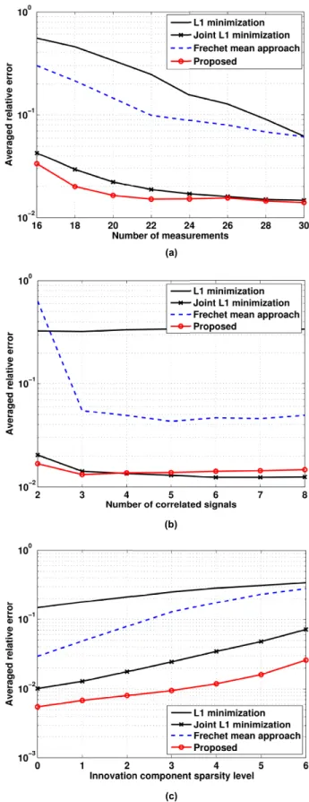
The reconstruction quality for different approaches is given in Fig. 2. In this experiment, we have compared the averaged relative error against number of measurements, number of signals and innovation component sparsity level. Comparing with conventional CS, i.e., performing independent ℓ1 min-imization, improved reconstruction quality is observed for the three approaches that exploit inter-signal correlations, and the proposed approach outperforms the other two joint reconstruction approaches. In addition, from Fig. 2 (c) we note that a high innovation component sparsity level results in a poor estimation quality of the common component by using the Fr´echet mean, and thus degrades the performance of the Fr´echet mean approach. However, the gain of the pro-posed approach is maintained for the case of high innovation component sparsity levels.
V. CONCLUSION
In this paper, we provide a Bayesian DCS framework for joint reconstruction of multiple correlated signals. An algorithm is proposed based on variational inference under the Bayesian DCS framework. The superiority of the proposed approach in relation to other existing approaches is revealed by our experimental study. Future work is to explore theoretical guarantees for the proposed approach.
ACKNOWLEDGMENT
The authors would like to thank Dr. David Wipf for gener-ously lending his expertise in a series of insightful discussions.
REFERENCES
[1] E. Cand`es, J. Romberg, and T. Tao, “Robust uncertainty principles: exact signal reconstruction from highly incomplete frequency information,” Information Theory, IEEE Transactions on, vol. 52, no. 2, pp. 489–509, 2006.
[2] D. Donoho, “Compressed sensing,”Information Theory, IEEE Transac-tions on, vol. 52, no. 4, pp. 1289–1306, 2006.
[3] R. Xie and X. Jia, “Transmission-efficient clustering method for wireless sensor networks using compressive sensing,”Parallel and Distributed Systems, IEEE Transactions on, vol. 25, no. 3, pp. 806–815, March 2014.
[4] W. Chen, M. Rodrigues, and I. Wassell, “A fr´echet mean approach for compressive sensing date acquisition and reconstruction in wireless sensor networks,” Wireless Communications, IEEE Transactions on, vol. 11, no. 10, pp. 3598 –3606, 2012.
[5] W. Chen and I. Wassell, “Energy-efficient signal acquisition in wireless sensor networks: a compressive sensing framework,” Wireless Sensor Systems, IET, vol. 2, no. 1, pp. 1–8, 2012.
[6] M. Duarte and Y. Eldar, “Structured compressed sensing: From theory to applications,”Signal Processing, IEEE Transactions on, vol. 59, no. 9, pp. 4053–4085, Sept 2011.
[7] M. Davies and Y. Eldar, “Rank awareness in joint sparse recovery,” Information Theory, IEEE Transactions on, vol. 58, no. 2, pp. 1135– 1146, Feb 2012.
[8] D. Baron, M. Wakin, M. Duarte, S. Sarvotham, and R. Baraniuk, “Dis-tributed compressed sensing,”Technical Report ECE-0612, Electrical and Computer Engineering Department, Rice University, Dec. 2006. [9] M. Duarte, M. Wakin, D. Baron, S. Sarvotham, and R. Baraniuk,
“Mea-surement bounds for sparse signal ensembles via graphical models,” Information Theory, IEEE Transactions on, vol. 59, no. 7, pp. 4280– 4289, 2013.
[10] D. Needell and J. Tropp, “Cosamp: Iterative signal recovery from incom-plete and inaccurate samples,”Applied and Computational Harmonic Analysis, vol. 26, no. 3, pp. 301 – 321, 2009.
[11] M. E. Tipping, “Sparse bayesian learning and the relevance vector machine,”The journal of machine learning research, vol. 1, pp. 211– 244, 2001.
[12] F. Chen, A. Chandrakasan, and V. Stojanovic, “Design and analysis of a hardware-efficient compressed sensing architecture for data compression in wireless sensors,”Solid-State Circuits, IEEE Journal of, vol. 47, no. 3, pp. 744–756, March 2012.
[13] F. Chen, F. Lim, O. Abari, A. Chandrakasan, and V. Stojanovic, “Energy-aware design of compressed sensing systems for wireless sensors under performance and reliability constraints,”Circuits and Systems I: Regular Papers, IEEE Transactions on, vol. 60, no. 3, pp. 650–661, March 2013. [14] R. Baraniuk, M. Davenport, R. DeVore, and M. Wakin, “A simple proof of the restricted isometry property for random matrices,”Constructive Approximation, vol. 28, no. 3, pp. 253–263, 2008.
[15] D. Wipf and B. Rao, “Sparse bayesian learning for basis selection,” Signal Processing, IEEE Transactions on, vol. 52, no. 8, pp. 2153–2164, Aug 2004.
[16] D. Wipf, B. Rao, and S. Nagarajan, “Latent variable bayesian models for promoting sparsity,”Information Theory, IEEE Transactions on, vol. 57, no. 9, pp. 6236–6255, Sept 2011.
[17] J. M. Winn and C. M. Bishop, “Variational message passing,” inJournal of Machine Learning Research, 2005, pp. 661–694.
[18] M. Grant and S. Boyd, “CVX: Matlab software for disciplined convex programming, version 2.0 beta,” http://cvxr.com/cvx, Sep. 2013.
(a)
(b)
(c)
Fig. 2. Comparison of reconstruction performance for different approaches. (a) reconstruction quality vs. number of measurements (n = 50,K = 4,
sc = 8and sI = 2); (b) reconstruction quality vs. number of correlated signals (n= 50,m= 25,sc= 10andsI= 1); (c) reconstruction quality vs. innovation component sparsity level (n= 50, m = 25, K = 4and