Galaxy Morphology and Evolution
by
Michael Andrew Peth
A dissertation submitted to The Johns Hopkins University in conformity with the requirements for the degree of Doctor of Philosophy.
Baltimore, Maryland May, 2016
c
Michael Andrew Peth 2016 All rights reserved
We can track the physical evolution of massive galaxies over time by characterizing the morphological signatures inherent to different mechanisms of galactic assembly. Structural studies rely on a small set of measurements to bin galaxies into disk, spheroid and irregular classifications. These classes are correlated with colors, SF history and stellar masses. Rare and subtle features that are lost in such a generic classification scheme are important for characterizing the evolution of galaxy mor-phology. We can connect the Hubble sequence observed for local galaxies to their high redshift progenitors to determine the full distribution of galaxy morphologies as a function of time over the entire lifetime of the Universe. To fully capture the complex morphological transformation of galaxies we need more useful classifications. To accomplish such a feat in a computationally tractable way we will need to convert galaxy images to low-dimensional representations of only a few parameters.
To overcome the limitations of the Hubble sequence, we use a principal component analysis of non-parametric morphological indicators (concentration, asymmetry, Gini coefficient,M20, multi-mode, intensity and deviation) measured at rest-frameB-band
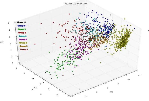
(corresponding to HST /W F C3 F125W at 1.4 < z < 2) to trace the natural distri-bution of massive (> 1010M) galaxy morphologies. Principal component analysis (PCA) quantifies the correlations between these morphological indicators and deter-mines the relative importance of each. The first three principal components (PCs) capture∼75% of the variance inherent to our sample. We interpret the first principal component (PC) as bulge strength, the second PC as dominated by concentration and the third PC as dominated by asymmetry. PC1 is a better predictor of quenching than stellar mass, as good as other structural indicators (S´ersic-n or compactness). We divide the PCA results into groups using an agglomerative hierarchical clustering method. Distinguishing between these galaxy structural types in a quantitative man-ner is an important step towards understanding the connections between morphology, galaxy assembly and star-formation.
Using a random forest classification technique, we are able to distinguish mergers from non-merger galaxies in Pan-STARRS imaging using a variety of input features (PCs, non-parametric morphologies, sSFR, M∗, rest-frame color). Determining if a galaxy is a merger is important to understand how influential mergers are in building bulges and assembling galaxies. The galaxies were initially visually classified by users of Galaxy Zoo. Asymmetry is by far the most important indicator of whether a galaxy is experiencing a merger. The next most important features include: PC7, PC5, PC3, deviation and d(G,M20). The importance of PC7 represents a very interesting result
a galaxy is a merger.
Galaxy simulations can provide valuable insight into the mechanisms behind galaxy evolution. The VELA simulations and subsequent non-parametric morpholog-ical measurements provide a resource to study the connection between morphology (through the use of PC results) and physical properties (such as sSFR, gas fraction, etc.). We stack the results of a discrete cross correlation between PCs and physical parameters from 9 VELA galaxies. Each of the first three PCs correlates differently with these physical parameters: PC1 is correlated strongly with ex-situ stellar mass, the gas fraction and sSFR; PC2 is weakly anti-correlated with all physical properties; PC3 is strongly correlated with sSFR at all length scales and with gas fraction in the central kpc. The process of star-formation, gas accretion and bulge assembly is a messy picture that will require more simulate galaxies to further understand the process of galaxy evolution.
Primary Reader: Dr. Jennifer Lotz (Space Telescope Science Institute) Secondary Reader:
I first need to thank my family: my mom, my dad, my sister and my grandma. All of you have been with me every step of the way. Without all the trips to the Air & Space Museum would I even be here writing this? There have been so many struggles along the way but each of you have kept me sane, kept me happy and made me feel loved. I have to thank my girlfriend, Ilana. No one has been able to help me believe in myself more than her. She has been a source of strength during the often difficult experience of writing this thesis and hunting for jobs.
I owe so much to my advisor Jennifer Lotz. Without her help, guidance and mentoring I would have been completely lost in graduate school. I feel like I won the lottery in terms of advisors. I couldn’t have asked for someone more patient, thoughtful and understanding. Not to mention she is one of the most intelligent people I’ve ever met and I am constantly in awe of how she is able to understand and dissect any topic in discussion. I owe a debt of gratitude to Gregory Snyder and Alireza Mortazavi. Our weekly group discussion were very helpful and insightful. I can trace the origins of a good chunk of this theses to comments and suggestions
made in those meetings. I also would like to thank our collaborators Peter Freeman and David Thilker who really provided me with the set of tools and impressive data (especially chapter 3). I need to thank my committee member and original co-advisor Harry Ferguson. I am very grateful to have been included in the CANDELS research team as I have been introduced to so many smart and interesting people, while also providing a chance to spread my scientific wings. None of this thesis would have been possible without contributions from those who crated the photometric, SED, visual morphology, VELA simulation and other assorted catalogs. I also need to thank my committee member Tamas Budavari who taught me so much about SQL, machine learning and data science in general in his course. I would like to thank the remainder of my thesis committee: Alex Szalay and Petar Maksimovic for reading my thesis, asking insightful questions and offering quality feedback. The thesis defense would not have been possible without the efforts of Jessica Rexroad and Kelley Key who really made it happen.
My fellow graduate students have been what has made this whole experience worth it. It all began with my friends who entered with me back in 2010: JT Mlack, Keith Redwine, Chris Martin, Kevin Grizzard and everybody else. We lived through the worst of the prelim exams, the POE and classes together, all while taking time to enjoy life and get together often. My 401 family (Raymond Simons, Rachael Alexandroff and Kirill Tchernyshyov) and the rest of the family tree (Duncan Watts, Roseanne Cheng, Erini Lambrides, David Jones and the rabble) hold a special place
in my heart. My 401 family has been a source of inspiration in my research but also have been a source of so many great experiences. No one will ever be able to top the homemade fried chicken found at Bones ’n’ Thrones. I truly would not be the person I am today without each of your friendships.
I thank the editors and anonymous reviewers of the Monthly Notices of the Royal
Astronomical Society who were very helpful in getting chapter 2 published as Peth
et al. (2016). This thesis used the following python libraries extensively: matplotlib, sci-kit learn, pandas, astropy, APLpy. I would like to thank the writers and main-tainers of these particular libraries for creating such quality products.
Lastly, I need to thank The Simpsons, Seinfeld, Curb Your Enthusiasm and The
Sopranos. When work became extremely stressful these shows provided me with some
much needed comfort. And thank you Radiohead for releasing new music right as work on this thesis reached a fever pitch.
When I heard the learnd astronomer;
When the proofs, the figures, were ranged in columns before me;
When I was shown the charts and the diagrams, to add, divide, and measure them;
When I, sitting, heard the astronomer, where he lectured with much ap-plause in the lecture-room,
How soon, unaccountable, I became tired and sick; Till rising and gliding out, I wanderd off by myself, In the mystical moist night-air, and from time to time, Lookd up in perfect silence at the stars.
Abstract ii
Acknowledgments v
Contents x
List of Tables xv
List of Figures xvii
1 Introduction 1
1.1 A Very Brief Overview of Galaxies . . . 1
1.2 Physical Mechanisms Causing Galaxy Evolution . . . 4
1.3 Galaxy Morphology as a Tool to Study Evolution . . . 9
1.4 Using Machine Learning to Analyze Galaxy Morphology . . . 12
1.5 Data Sets Used in This Analysis . . . 16
Structure at 1.4 < z < 2 via Principal Component Analysis 19
2.1 Introduction . . . 19
2.2 Data . . . 22
2.2.1 Sample Selection Criteria . . . 23
2.2.2 Galaxies with FLAG=1 . . . 25
2.3 Morphological Measurements . . . 25 2.3.1 Non-parametric Morphology . . . 25 2.3.1.1 Petrosian Radius . . . 27 2.3.1.2 Concentration . . . 27 2.3.1.3 Asymmetry . . . 28 2.3.1.4 Gini Coefficient . . . 29 2.3.1.5 M20 . . . 31 2.3.1.6 Multi-mode . . . 32 2.3.1.7 Intensity . . . 33 2.3.1.8 Deviation . . . 34
2.3.2 Morphological Principal Components . . . 34
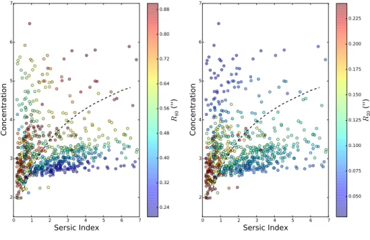
2.3.3 Concentration - S´ersic Index Relationship . . . 37
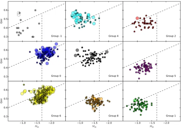
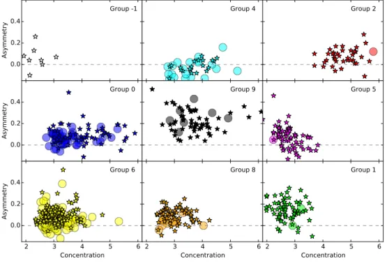
2.4 PCA-Morphology Group Properties . . . 48
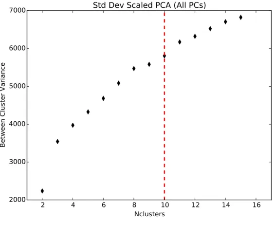
2.4.1 Defining PCA morphology groups . . . 48
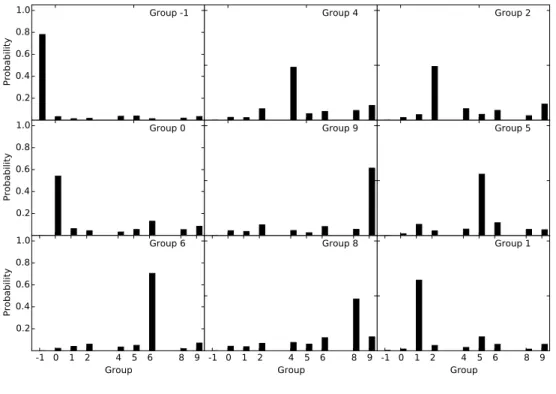
2.4.2 Morphological Error Estimation . . . 50
2.6 Discussion . . . 74
2.6.1 Stellar Mass - Quenching Connection for groups . . . 76
2.6.2 The relationship between PCA Classes and Visual/S´ersic Clas-sifications . . . 77
2.6.2.1 The Compact and Bulge-Dominated Galaxies: Groups 0, 6 and 9 . . . 78
2.6.2.2 The Disk-dominated Galaxies: Groups 1, 2 and 5 . . 80
2.6.2.3 The Intermediate Galaxies: Groups 4 and 8 . . . 81
2.6.2.4 Comparing the Irregular Galaxies of Groups 1 and 9 82 2.7 Summary . . . 84
3 Merger Classifications of Pan-STARRS Galaxies Using Random For-est 96 3.1 Introduction . . . 96
3.2 Data . . . 101
3.2.1 Ground Based Surveys: Pan-STARRS and SDSS . . . 101
3.2.2 Galaxy Zoo . . . 102
3.3 Non-parametric Morphology of Pan-STARRS Galaxies . . . 105
3.3.1 Principal Component Analysis of PanSTARRS Galaxies . . . 108
3.4 Random Forest Classifier . . . 115
3.4.1 Random Forest Inputs . . . 120
3.5.1 Random Forest Classifications . . . 121
3.5.1.1 Random Forest Input Parameter Tests . . . 123
3.5.1.2 Comparisons of RF on Different Subsamples . . . 130
3.6 Discussion . . . 140
3.6.1 Random Forest Classifications of MaNGA Galaxies . . . 140
3.7 Summary and Conclusions . . . 142
4 VELA Simulation Galaxy Morphologies 148 4.1 Introduction . . . 149
4.2 Data . . . 156
4.2.1 VELA Simulation . . . 156
4.2.2 Image Processing and CANDELization . . . 158
4.3 PCA-Morphology Groups . . . 160
4.3.1 PC Group Demographics . . . 161
4.3.2 PC Group Flow . . . 165
4.4 Time Series Cross-Correlations . . . 175
4.4.1 Discrete Correlation Function . . . 179
4.4.2 Stacks of PCs and Physical Parameters Correlations . . . 188
4.5 Discussion . . . 212
4.5.1 Is PC1 an indicator of evolution? . . . 213
4.5.2 How PC2 interacts with galaxy evolution . . . 216
4.6 Summary . . . 219
5 Summary and Future Directions 222 5.1 Galaxy Morphological Classifications Using PCA . . . 223
5.2 Random Forest Classifications of Pan-STARRS Galaxies . . . 224
5.3 Studying Galaxy Morphology Using VELA Simulation Suite . . . 226
5.4 Mergers Can Grow Bulges and Regulate Star-formation . . . 227
5.5 Future Work . . . 230
Bibliography 233
2.1 PC Weights with error estimates based on a bootstrap scattering method 38 2.2 Group percentages by mass range for both original group and “MC
Group” . . . 63
2.3 Demographics of Visual Classifications of Groups . . . 64
2.4 Demographics of S´ersic Classifications of Groups . . . 65
2.5 U V J Quenched Fractions of Groups . . . 66
3.1 Feature Importances of RF Classifications . . . 128
3.2 Feature Importances of RF Classifications . . . 129
3.3 Summary Statistics of RF Classifications . . . 135
3.4 Summary Statistics of RF Classifications . . . 136
3.5 False Positive Examples . . . 145
4.1 VELA PCA Group Demographics at all viewing angles. The CAN-DELS sample is shown for comparison. . . 166
4.2 VELA PCA Group Demographics by Camera Angle. CAMERA0 rep-resents the face-on view and CAMERA1 reprep-resents the edge-on view. The remaining cameras are from random angles. The CANDELS sam-ple is shown for comparison. . . 167
2.1 Histogram of F125W J-band Magnitude for galaxies with FLAG=1
and FLAG=0 . . . 26
2.2 Example of M ID statistics . . . 30
2.3 Concentration - S´ersic index for sample . . . 41
2.4 Concentration - S´ersic Including PSF Effects . . . 42
2.5 PC1 vs Sersic Index and Gini-M20 Bulge Strength . . . 43
2.6 3D PC1-PC2-PC3 color-coded by group . . . 44
2.7 Between cluster variance vs. N clusters . . . 45
2.8 Magnitude vs. ∆(GOODS - UDF) morphological statistics . . . 46
2.9 Magnitude vs. ∆(GOODS - UDF) morphological statistics . . . 47
2.10 Group classification uncertainty . . . 51
2.11 Rest-frame U V J . . . 52
2.12 Rest-frame U −V vs. Stellar Mass . . . 56
2.13 Gini – M20 . . . 57
2.15 Effective radii (kpc) - M∗ . . . 59
2.16 Cumulative quenched fraction rank . . . 75
2.17 Group 6 F125W 1.36 <z < 1.97 galaxies . . . 87 2.18 Group 0 F125W 1.36 <z < 1.97 galaxies . . . 88 2.19 Group 9 F125W 1.36 <z < 1.97 galaxies . . . 89 2.20 Group 4 F125W 1.36 <z < 1.97 galaxies . . . 90 2.21 Group 8 F125W 1.36 <z < 1.97 galaxies . . . 91 2.22 Group 1 F125W 1.36 <z < 1.97 galaxies . . . 92 2.23 Group 2 F125W 1.36 <z < 1.97 galaxies . . . 93 2.24 Group 5 F125W 1.36 <z < 1.97 galaxies . . . 94 2.25 Group -1 F125W 1.36 <z <1.97 galaxies . . . 95
3.1 Galaxy Zoo Decision Tree . . . 106
3.2 Gini - M20 for PANSTARRS Mergers . . . 109
3.3 Concentration - Asymmetry for PANSTARRS Mergers . . . 110
3.4 Concentration - Asymmetry for PANSTARRS Mergers . . . 111
3.5 PC1-PC2-PC3 Plot for PANSTARRS Galaxies . . . 113
3.6 Histogram of PC groups for CANDELS and Pan-STARRS . . . 114
3.7 Visualization of Random Forest Part 1 . . . 118
3.8 Visualization of Random Forest Part 2 . . . 119
3.9 Gini-M20 color-coded by RF Classification Probabilities . . . 124
3.11 Concentration-Asymmetry color-coded by RF Classification Probabilities126 3.12 Concentration–Asymmetry coded by RF Classification Confusion Matrix127 3.13 OOB Errors for Random Forests Using Different Numbers of Max Leaf
Nodes . . . 131
3.14 Summary Statistics for Random Forests Using Different Max Leaf Nodes132 3.15 ROC Curve . . . 133
3.16 Feature Importance Comparisons between Blue and Red Galaxies . . 137
3.17 Feature Importance Comparisons between Merged Galaxies and Merg-ing Pairs . . . 138
3.18 Feature Importance Comparisons between the Full Sample and Blue/Red, Merged Galaxies/Merging Pairs . . . 139
3.19 Images of False Positives . . . 143
3.20 Segmentation Maps of False Positives . . . 144
4.1 PC group histogram of VELA galaxies . . . 168
4.2 Gini–M20 of VELA galaxies . . . 169
4.3 Concentration–Asymmetry of VELA galaxies . . . 170
4.4 PC group histogram of VELA galaxies with Asym Correction . . . . 171
4.5 PC group histogram of minor mergers . . . 172
4.6 PCgroup(z) for all VELA galaxies . . . 176
4.7 fgas(t) for all VELA galaxies . . . 177
4.9 PC2 for all VELA galaxies . . . 190
4.10 PC3 for all VELA galaxies . . . 191
4.11 sSFR for all VELA galaxies . . . 192
4.12 fgas for all VELA galaxies . . . 193
4.13 ˙fgas for all VELA galaxies . . . 194
4.14 ex-situ M∗ for all VELA galaxies . . . 195
4.15 ex-situ ˙M∗ for all VELA galaxies . . . 196
4.16 M˙dm for all VELA galaxies . . . 197
4.17 sSFR-PC1 Cross-correlation for VELA02 . . . 198
4.18 Gas Fraction - PC1 Cross-correlation for VELA02 . . . 199
4.19 Rate of gass mass into central kpc - PC1 of VELA02 . . . 200
4.20 Ex-situ stellar mass into central kpc - PC1 of VELA02 . . . 201
4.21 Rate Ex-situ stellar mass into central kpc - PC1 of VELA02 . . . 202
4.22 Rate of DM mass into central kpc - PC1 of VELA02 . . . 203 4.23 Stack of cross-correlations for PC1 - physical parameters for inner kpc 206 4.24 Stack of cross-correlations for PC1 - physical parameters for total galaxy207 4.25 Stack of cross-correlations for PC2 - physical parameters for inner kpc 208 4.26 Stack of cross-correlations for PC2 - physical parameters for total galaxy209 4.27 Stack of cross-correlations for PC3 - physical parameters for inner kpc 210 4.28 Stack of cross-correlations for PC3 - physical parameters for total galaxy211
Introduction
1.1
A Very Brief Overview of Galaxies
Initially after the Big Bang, the Universe was in a state of near but not perfect homogeneity with small quantum fluctuations present throughout. Following a period of rapid expansion in the Universe, known as inflation, these quantum fluctuations became amplified into regions of higher and lower density. At this point the Universe was radiation dominated and all primordial elements (such as hydrogen) were fully ionized. However, the ionized photons could not travel very far without Thomson scattering off a free electron. The continuing expansion cooled the Universe enough that it became energetically possible for protons and electrons to combine and form neutral hydrogen. This era, known as recombination (or decoupling), brought about the opportunity for baryonic matter assembly. Photons became decoupled from the
formerly charged particles and became free to propagate throughout the universe. These photons are visible as the Cosmic Microwave Background (CMB). The CMB is nearly uniform except for slight temperature fluctuations on the order of 10−5 K
(Bennett et al., 2013; Mather et al., 1990; Planck Collaboration et al., 2014). These temperature fluctuations are the evidence of the density fluctuations of the post-inflation Universe.
The standard model of cosmology, known as Lambda-Cold Dark Matter (ΛCDM), posits the existence of “dark energy” which is responsible for counteracting the at-tractive effects of gravity and “cold dark matter” that only interacts with itself and other particles through gravity and does not radiate photons. Dark matter clumps grew from the perturbations in the density distribution of the Universe.
Dark matter is able to collapse in a dissipational manner (does not radiate away energy through photons) due to to gravity and forms halos. The smallest dark matter halos are able to form first, later merging with one another to create progressively larger halos (White & Rees, 1978). This growth of dark matter halos is known as hierarchical assembly and is central to ΛCDM cosmology. Baryonic matter (in the form of gas) is accreted by these halos at which time the gas cools and fragments to form galaxy structures. Eventually, dark matter halos accrete enough gas to form what we know of as galaxies.
Galaxies can continually accrete material either smoothly or stochastically from the surrounding intergalactic medium. Smooth accretion in the form of cold gas
dis-tributed along dark matter filamentary structure is directly dumped onto the galaxy (Birnboim & Dekel, 2003; Dekel et al., 2009b). These so-called cold streams are among the main sources of gas for higher redshift galaxies (Dekel et al., 2009b). Stochastic accretion can occur in the form of merging galaxies (see §1.2).
Modern cosmological simulations (such as Illustris Vogelsberger et al., 2014 and EAGLE McAlpine et al., 2015) have successfully reproduced how observed galaxies form and grow in dark matter halos through the constant collapse of molecular clouds into stars and the gravitational attraction to form increasingly complex structures (Springel et al., 2005).
The most widely used visual classification scheme, the Hubble sequence, divides galaxies into ellipticals (also known as early-type galaxies), transitionary phase (known as lenticular galaxies) and spiral galaxies (also known as late type galaxies) (Hubble, 1926). The elliptical galaxies vary in elongation from round to triaxial shapes and have smooth light profiles, star follow random orbits and appear spheroidal. The spiral galaxies consist of stars orbiting rotationally in spiral structures are subdivided by how tightly wound the spiral arms are and is a central bar exists. Typically the spectral color of a galaxy is related to the morphology: elliptical galaxies are com-posed of red and old stars, while spiral galaxies are comcom-posed of blue and young stars. Galaxies not fitting into this scheme are labeled as irregular. Irregular galaxies can be low mass galaxies or the result of the merger of two galaxies.
way they do? What physical mechanisms build galaxies into these specific structures and either create a large number of stars or prevent stars from forming?
1.2
Physical Mechanisms Causing Galaxy
Evolution
There exists a strong correlation between the rate of star-formation and the amount of stellar mass, known as the “main sequence of star formation” as far back asz ∼2.5 (Noeske et al., 2007; Wuyts et al., 2011). In this correlation, there exists a bi-modality in star-formation and stellar mass that is highly correlated with color and morphological type. Blue, star forming, primarily disk galaxies have star-formations and masses that follow a very tight relationship (e.g. Baldry & Glazebrook, 2003; Hogg et al., 2004; Bell et al., 2004). Meanwhile, red, low star-formation, primarily spheroidal galaxies fall below this relationship and have less star-formation than a bluer galaxy has for a specific mass and redshift. Galaxies with star-formation below the main sequence are known as “quenched”.
During the epoch known as “cosmic high noon” (z=1.5 – 3), the cosmic star formation rate is at a maximum and at which time nearly half of all stellar mass assembles (Madau & Dickinson, 2014). Galaxies were forming more stars per unit mass at higher redshift (Noeske et al., 2007). Even at this epoch, massive galaxies (M∗ >1010 M) begin to experience declining star formation, which is coupled with
an emergence of red central bulges (Kriek et al., 2006; van Dokkum et al., 2008; Kriek et al., 2009; Whitaker et al., 2012). Since “cosmic high noon” there has been a dramatic increase in the number of high mass quenched galaxies observed (e.g. Faber et al., 2007; Bell et al., 2012).
Any discussion of the overall galaxy morphology and star-formation characteristics would be incomplete without a discussion of bulges. Not all bulges are created equal, there are a few different structures which may collectively be called “bulges” but which are different from one another. There are “classical” bulges which resemble giant elliptical galaxies, but exist at the center of disk galaxies. The stars in these bulges are on random orbits and are redder than the stars in the disk. The light distribution is well described by the de Vaucouleurs law (surface brightness∝r1/4). A classical bulge is likely the final stage of the merger of two disk galaxies (Toomre, 1977; Kormendy & Kennicutt, 2004). Additionally, there are “pseudo-bulges” which are spheroidal and exist at the center of disk galaxies, however the stars orbit the center rotationally (similar to the outer disk). Pseudo-bulge light profiles are not well described by the de Vaucouleurs profile and are instead better fit by a Sersic profile (∝ r). Pseudo-bulges are likely the result of internal galaxy interactions such as bars and spiral structure (Kormendy & Kennicutt, 2004). Understanding the difference between these two types of bulges can have an impact on the likely formation mechanisms for a particular galaxy.
(r.1–3 kpc) galaxies can resemble local elliptical galaxies but are actually a separate class, known as “compact” galaxies. Compact galaxies likely formed via gas inflows towards the central region of the galaxy. Quenched compact galaxies can have radii of 1 kpc or smaller (van der Wel et al., 2014a). Many z∼3 galaxies are compact elliptical galaxies with low amounts of star formation (van Dokkum et al., 2008, 2010; Whitaker et al., 2012). Compact, star forming galaxies have similar masses, kinematics, and abundances as quenched, red compact galaxies and are the likely progenitors (Barro et al., 2013, 2014b; Williams et al., 2014). Both types of compact galaxies are seen in hydrodynamical (Ceverino et al., 2014; Wellons et al., 2015) and semi-analytic (Brennan et al., 2015) simulations.
Why galaxies experience this reduction in star formation and bulge formation is hotly debated. Observations reveal a cosmic transition from blue and star form-ing disk galaxies to red and quenched spheroidal galaxies leadform-ing to an interestform-ing “chicken or egg” problem: Do galaxies experience a morphological transformation that quenches star formation, or does star formation quenching lead to a fading disk? The mechanisms quenching star formation and affecting the morphology of galaxies are not fully understood but can be explained in a few different ways: major/minor mergers (e.g. Naab et al., 2006a; Hopkins et al., 2010); feedback from active galactic nuclei (AGN; e.g. Croton et al., 2006; Somerville et al., 2008a); secular processes (such as the spiral bar instabilities, star formation, gas recycling Kormendy & Kennicutt, 2004; Bournaud et al., 2007; Elmegreen et al., 2008; Genzel et al., 2008).
Mergers are are defined by their mass ratios (major or minor) and their gas content (gas-rich or “wet” and gas-poor or “dry”). Each type of merger can influence star-formation and morphology in a different manner.
Major mergers (collisions between galaxies of roughly equivalent mass, mass ratio of.1:3) can destroy disks by the gravitational interactions of the constituent galaxies and eventually reassemble into a relaxed spheroid. Galaxies with significant gas fractions interact which leads to peculiar features such as tidal tails, asymmetries, double nuclei, rings, shells (Toomre & Toomre, 1972). Major gas-rich galaxy mergers rapidly funnel gas into the cores of massive galaxies and feeds bulges (e.g. Sanders & Mirabel, 1996; Heckman et al., 2004). Gas-rich mergers provide a supply of star-forming fuel which can lead to starburst activity. Meanwhile, Gas-poor mergers are primarily responsible for the mass and size evolution of spheroids at z < 2 (Naab et al., 2006a, 2009).
Minor mergers (which are generally between galaxies with a mass ratio of >1:10) may also disrupt morphologies, and gas-poor minor mergers must be more frequent than major mergers (Lotz et al., 2011; Papovich et al., 2012). Peculiar properties, such as low surface brightness tidal features, are often difficult to detect and require deep observations. The primary galaxy accretes stellar material from the satellite onto the outskirts (e.g. Naab et al., 2006b; Bell et al., 2006). Even the small amount of gas accreted in a minor merger is sufficient to trigger an AGN or starburst, and eventually quench star-formation (Kormendy & Richstone, 1995; Croton et al., 2006;
Somerville et al., 2008b).
Internal mechanisms, collectively referred to as secular processes, include the in-teractions of bars in a spiral galaxy rearranging disk gas (Kormendy & Kennicutt, 2004), and violent disk instabilities (VDIs, Kereˇs et al., 2005) leading to enhanced star-formation, irregular morphologies, angular momentum loss, rapid star-formation and supermassive black hole (SMBH) growth (Magorrian et al., 1998; Ferrarese & Merritt, 2000; Shankar et al., 2012; Elbaz & Cesarsky, 2003). In this scenario, the morphology of the galaxy is unaffected and the galaxy appears undisturbed and disk-like (Simard & Pritchet, 1998; Schawinski et al., 2011). Once the reservoir of gas is exhausted and star-formation is quenched, a disk structure can still exist.
Slow, long-term quenching mechanisms are required to keep galaxies quenched (Barro et al., 2013). This quenched state can be maintained by mechanisms such as mass quenching (Dekel & Birnboim, 2006; Bell et al., 2012) which is caused by the halo growing above a threshold mass of 1011M. At this mass, shocks are created which do not allow gas to cool sufficiently to form stars. Quenching can also maintained by a sufficiently massive central bulge stabilizing the disk from further fragmentation and thus shutting down star formation (morphological quenching; Tacchella et al., 2015; Martig et al., 2009; Genzel et al., 2014). Additionally, AGN can provide strong jets that can heat the surrounding halo and thus prevent gas to cool and form stars (Cattaneo et al., 2009). On the other hand bulges, by themselves, have proven to be a “necessary but not sufficient” mechanism to shut down star-formation (Bell et al.,
2012; Fang et al., 2013).
Each mechanism leaves behind different clues (in the shape and structure of galax-ies). Can we determine which mechanisms are important for a specific type of galaxy during a specific cosmic epoch? A possible answer is in the morphology of a galaxy. The shape and structure can tell us what processes have been important during a galaxy’s history.
1.3
Galaxy Morphology as a Tool to Study
Evolution
Morphology can offer clues that indicate how responsible mergers (and other mech-anisms) are (or are not) in quenching galaxies and building bulges. Morphological classes (such as spheroids and disks) are correlated with colors, star-formation his-tory and stellar masses. Significant correlations have been observed between star-formation rate, stellar mass and quantitative morphological measurements (Wuyts et al., 2011).
To study the processes driving evolution, we need a method to effectively and efficiently characterize the structures and shapes of galaxies. Visual classifications (such as the Hubble sequence) have been used since the discovery of galaxies, and have subsequently been adapted to fit modern surveys (e.g. Galaxy Zoo, Lintott et al., 2008a; Kartaltepe et al., 2015). These visual studies rely on the Hubble sequence to
classify galaxies and will have classifiers place galaxies into disk, spheroids, irregular and unknown categories. Visual classifications can find subtle structural elements possibly missed by an automated routine. However, human classifications of galaxies can be very time consuming and subjective.
However, galaxy structure at high redshift does not always correspond to the local Hubble sequence (Bruce et al., 2012; Bell et al., 2012; Kriek et al., 2009; Lee et al., 2013). Disk-dominated galaxies can appear clumpy (F¨orster Schreiber et al., 2009) and spheroid-dominated galaxies can be compact, very red and massive, but possess no extended envelope (e.g. van Dokkum et al., 2008). Therefore the standard Hubble sequence will miss rare and subtle features inherent to the morphology of high redshift galaxies and may need updating for high redshift.
Galaxies can appear vastly different between UV and optical wavelengths (e.g., Meurer et al., 1995). UV light traces bright stars and thus active star formation (since these stars are short-lived). Meanwhile, optical wavelengths longer than the Balmer (400 nm) break observe stars at a variety of ages. Progressively older stars dominate the galaxy spectral energy distribution (SED) at longer wavelengths. Additionally, dusty galaxies can have much of their optical light absorbed (Calzetti et al., 2000) and reradiated in the IR. To combat these wavelength-dependent morphological conditions it is important to observe galaxy morphology at a single rest-frame wavelength across redshift.
defining morphology have been created. The relationship between surface brightness and radius for elliptical galaxies (I ∝ r1/4) was first determined by de Vaucouleurs (1948). The de Vaucouleurs law was eventually generalized by Sersic (1968) to a S´ersic profile (I ∝ r1/n) with disk galaxies of n=1. Later studies decomposes the galaxy
into bulge and disk profiles (Kormendy, 1977b) for even further discriminatory power between disks and bulge dominated galaxies. Many studies (e.g. Bell et al., 2012; van der Wel et al., 2012) fit a S´ersic profile to a galaxy for the purposes of classification.
GALFIT (Peng et al., 2002, 2010) is an automated technique often used to classify galaxies by fitting the galaxy light distribution to a S´ersic profile (r−1/n) and is
sen-sitive to small galaxies, can distinguish overlapping light profiles of nearby galaxies, incorporates the point spread function of a specific field/detector, and most impor-tantly is easy to interpret. However, GALFIT assumes a symmetric and smooth light profile, which at times can be problematic. This assumption does not hold for irreg-ular galaxies, merger remnants, and disk galaxies with bars or clumps.
Quantitative non-parametric morphological statistics characterize galaxy struc-ture and do not assume an analytic light profile. This fact allows us to apply au-tomated characterization to irregular galaxies as well. Examples of non-parametric morphological indicators include: concentration index (C, Bershady et al., 2000; Con-selice et al., 2003), asymmetry (A, Conselice et al., 2000), Gini coefficient (G, Abra-ham et al., 2003; Lotz et al., 2004), M20 (Lotz et al., 2004), and three new statistics
M IDstatistics have been found to be the most sensitive to mergers and clumpy star-formation, even at high redshift (Freeman et al., 2013). CASis capable of identifying major mergers, while Gini–M20 can identify both major and minor mergers (just not
to the same extent as the M ID statistics, Conselice, 2014).
However, for many galaxies these statistics can be strongly correlated. Moreover, cosmological models of galaxy formation yield a picture in which these structures can evolve quickly along diverse paths, thereby motivating the need for a broad classifi-cation system (Snyder et al., 2015a). Therefore we require further analysis to under-stand the inherent relationships among these statistics and between galaxy assembly processes.
1.4
Using Machine Learning to Analyze
Galaxy Morphology
In the upcoming years and decades, many new telescopes and surveys will become operational; such as the Large Synoptic Sky Telescope (LSST; Ivezi´c et al., 2008), the European Extremely Large Telescope (E-ELT), the Thirty Meter Telescope (TMT), and the Dark Energy Survey (DES), among others. Each of these telescopes will produce terabytes to petabytes of observational data nightly. Novel data analysis strategies will need to be created to account for the sheer deluge of information. These massive data sets will provide significant insights into every aspect of astrophysics to
a degree that only a decade ago may have seemed outlandish.
The sheer amount of images from future telescope surveys will make human visual classifications of galaxies an intractable problem. However, machine learning tech-niques are often successful at reproducing many of the results. In their review of data mining in astronomy, Ball & Brunner (2010), state the advantages as follows: sim-plicity, influence from prior information, pattern recognition, complimentary analysis and the simple ability to “get anything at all”. Complimentary analysis refers to the idea that different approaches to a problem will reduce the systematic errors inherent to any single approach.
To make sense of all this data, astronomers have begun to implement machine learning and data mining into their analysis. Data mining is simply a collection of techniques useful for analyzing and describing structured data (Ivezi´c et al., 2013). These techniques include: principal component analysis (PCA), clustering, unsu-pervised classification, amongst many others. Machine learning refers to a set of techniques that compare datasets to previously understood sets. These techniques include: random forest (RF), support vector machines (SVM), artificial neural net-works (ANN) and maximum likelihood estimator.
There are two broad categories of machine learning techniques: supervised and unsupervised. Unsupervised techniques (such as principal component analysis, see Chapter 2) are helpful to reduce the dimensionality of a problem and to find rela-tionships amongst the data. Supervised learning techniques, such as random forest
(Breiman, 2001), support vector machines (Vapnik & Vapnik, 1998), and artificial neural networks (ANN; Ripley, 1981, 1988), use a training set of labeled data to build a framework for which to classify unlabeled data.
Principal component analysis (PCA) is a simple way to reduce the dimensionality, break internal degeneracies and find the natural distributions of data in parameter space. To eliminate degeneracies inherent in these morphological statistics we per-formed a PCA using 7 non-parametric morphology measurements on 1244 galaxies from 1.36 < z < 1.97. PCA has been shown to efficiently classify galaxies (e.g. Taghizadeh-Popp et al., 2012; the Zurich Estimator of Structural Types (ZEST), Scarlata et al., 2007a). A few studies immediately capitalized on the ZEST classifica-tions to study the number density evolution of disk galaxies (Sargent et al., 2007), the luminosity function evolution for elliptical galaxy progenitors (Scarlata et al., 2007b), and the evolution of the galaxy merger rate toz ∼ 1 (Kampczyk et al., 2007).
The Zurich Estimator of Structural Types (ZEST; Scarlata et al., 2007a) uses a PCA of 5 non-parametric morphological diagnostics: Gini coefficient, M20,
concen-tration, asymmetry, and ellipticity. They classify ∼56,000 bright (IAB < 24)
COS-MOS into spheroidal, disk and irregular galaxy types while additionally calculating a bulginess, elongation, irregularity and clumpiness parameter for each galaxy. The classifications are used to demonstrate redshift evolution (since z∼1) of the galactic luminosity function (LF) for galaxies of different classes. Their analysis concluded that the average volume density of disk galaxies remains constant. However, the
stel-lar populations of these systems are brightened at earlier epochs. Only the bright, (MB < -21.5) end of the irregular and the early-type galaxies remains roughly
con-sistent with the LF of local galaxies. At fainter magnitudes, irregular and early-type galaxies show evolution from z = 0 to 0.7.
Similarly, Taghizadeh-Popp et al. (2012) uses PCA to describe the entire zoo of galaxy morphologies with a single parameter. Which they derived from a set of ob-servational derived quantities: mass-to-light ratio, surface brightness, concentration, star-formation rate, specific star-formation rate, g-r and u-r. Their analysis labels, ranks and classifies galaxies by a single arc-length value.
Supervised methods such as random forest have been used to classify galaxies (e.g. Lahav et al., 1995; Freeman et al., 2013). The random forest technique was developed by Breiman (2001) as a supervised method for classification. The random forest classifier is learned from a labeled training set representing a random sample of the total sample. The split best differentiating mergers from non-mergers among the random subset of the features in each node defines the optimal classifiers. Random forest inherently provides probabilities which we can use to investigate the effect thresholds have on the completeness and quality of classifications.
Supervised techniques require a basis set of data in which all subsequent classifi-cations are founded upon. Freeman et al. (2013) uses the CANDELS visual classifica-tions (Kartaltepe et al., 2015) to build a classification schema out of non-parametric morphologies for separating mergers from non-mergers. The M, I, and D statistics
are more useful than Gini and M20 at identifying disturbed morphologies. Lahav
et al. (1995) compared visual classifications of galaxies by world experts (such as de Vaucouleurs) to classifications by an Artificial Neural Network. The Sloan Digital Sky Survey was used as a training set (over 143 million objects) to separate galaxies from stars (Ball et al., 2004). Huertas-Company et al. (2015) uses convolutional neural networks to classify galaxies based on non-parametric morphological measurements from CANDELS.
Supervised techniques are not just used to classify galaxies but can be used to infer values such as photometric redshifts and galaxy stellar masses. Kamdar et al. (2016a,b) use random forest regression of semi-analytic models of galaxies to make predictions of observable galaxy properties from pure dark matter simulations. Carliles et al. (2010) uses random forest trained upon SDSS galaxies to calculate photometric redshifts.
1.5
Data Sets Used in This Analysis
The Cosmic Assembly Near Dawn Extragalactic Legacy Survey (CANDELS, PIs: S. Faber and H. Ferguson; Grogin et al. 2011 and Koekemoer et al. 2011) provides a wealth of data from 5 heavily studied fields (UDS, EGS, COSMOS and GOODS-North+South) with observations by the Hubble Space Telescope (HST). Space based observations from HST provide the highest resolution ever for a sample of high
red-shift galaxies . High resolution is critical for observations of low surface brightness structural features. Without which, morphological evolution would be incredibly dif-ficult. Observations by the Wide Field Camera 3 (WFC3) in Near-Infrared bands, F125W (J) and F160W (H), combined with observations from the Advanced Camera for Surveys (ACS) in UV-Visible bands, F814W (i) and F606W (V) constitute the new measurements in the CANDELS program.
We focus on high mass (M∗ > 1010 M) galaxies, brighter than H < 24.5. We restrict ourselves to only redshift ranges that correspond our observed morphologies to a single rest-frame waveband. Constant rest-frame morphologies are crucial for understanding possible evolution in the stellar structures of galaxies while preventing strong wavelength, and therefore redshift biases.
High redshift observations can be extended to low redshifts through the use of large all sky surveys. In the next few years, the Panoramic Survey Telescope and Rapid Response System (Pan-STARRS) will provide a dataset of up to 50,000 galaxies (with an addition 3,000 from a Medium Deep Survey) that will need to be analyzed. Pan-STARRS will take frequent and repetitive wide-field images over nearly the entire visible sky. Additionally, the Sloan Digital Sky Survey (SDSS; York et al., 2000a), is a very well established program that has observed over a million low redshift galaxies. The observations of low redshift galaxies from SDSS and PAN-STARRS will offer a critical baseline for comparison to the high redshift galaxies from CANDELS.
moderately massive galaxies calculated using Eulerian gas dynamics and an N-body Adaptive Refinement tree (ART, Kravtsov et al., 1997; Kravtsov, 2003). The VELA simulations are described in depth by Ceverino et al. (2010a); Ceverino & Klypin (2009); Ceverino et al. (2012); Dekel et al. (2013); Ceverino et al. (2014). The simula-tion outputs have been processed (usingSUNRISEJonsson, 2006; Jonsson et al., 2010 and CANDELization Mozena, 2013) to resemble observed galaxies at high redshift by CANDELS (Snyder et al., 2015b). The VELA simulations offer a new avenue to study individual galaxy evolution from 1 . z . 3 and how physical processes are directly related to morphology.
Beyond Spheroids and Discs:
Classifications of CANDELS
Galaxy Structure at 1.4
< z <
2 via
Principal Component Analysis
2.1
Introduction
Massive galaxies today form stars at a lower rate than in the past due to many factors. However, we do not have a complete accounting of the processes quenching the star-formation in galaxies. An increase in the mass/number densities (Tomczak et al., 2014; van der Wel et al., 2014b) of massive, red galaxies implies stars are not
forming to the same extent they once were. Each of these observations attempt to connect of observed color (or star-formation rate) and stellar masses to morphology. The star-formation rate - stellar mass (SFR−M∗) relationship shows star-forming galaxies at z ∼ 0 follow a “main sequence” (Brinchmann et al., 2004; Wuyts et al., 2011). Galaxies on the main sequence are bluer and have lower S´ersic-indices than galaxies below the relation. Massive galaxies with low SFRs are red and have high S´ersic indices and bulge strengths. The SFR−M∗ morphology relation has been shown to hold out toz ∼ 2.5 (Wuyts et al., 2011). However, bulge strength has been described as a “necessary but not sufficient” condition for quenching star-formation inz . 2.2 galaxies (Bell et al., 2012).
If the presence of a bulge is not sufficient to fully quench a galaxy, other factors such as size may be important for shutting down star-formation. At redshifts z ∼ 1.5, galaxies of sufficiently high mass and small size are quenched (Barro et al., 2013). This suggests a relationship between so-called “compactness” (Σ1.5 =M/re1.5) and the
specific star-formation rate (sSFR) . However, the number density of these compact galaxies has been decreasing with the age of the Universe.
The mechanisms for quenching star-formation and transforming the morphology of galaxies are not fully understood. Proposed mechanisms include: major mergers (e.g. Naab et al., 2006a; Hopkins et al., 2010); minor mergers (e.g. Taniguchi, 1999; Hopkins & Hernquist, 2009; Villforth et al., 2013); secular processes (for review see Kormendy & Kennicutt, 2004; Cisternas et al., 2011); AGN feedback (e.g. Silk &
Rees, 1998; Schawinski et al., 2006); and mass quenching (Dekel & Birnboim, 2006; Bell et al., 2012). Comprehensive models of galaxy formation can yield a reasonable link between galaxy morphology and star formation (e.g. Snyder et al., 2015b) but we do not yet have a perfect accounting of how all these processes might contribute. As a result, two evolutionary tracks have been developed to explain the disappear-ance of compact, quenched galaxies: (1) major mergers at z ∼ 2-3 quickly cause a galaxy to quench, which later grow through minor mergers and gas accretion; (2) vio-lent disk instabilities/secular processes/minor mergers at z∼1.5 cause a slower decline in star-formation and simultaneous size growth before the quiescent phase.
To study the processes driving evolution, we need a method to effectively and efficiently characterize the structures and shapes of galaxies.
Quantitative non-parametric morphological statistics characterize galaxy struc-ture and do not assume an analytic light profile. This fact allows us to apply au-tomated characterization to irregular galaxies as well. Examples of non-parametric morphological indicators include: concentration index (C, Bershady et al., 2000; Con-selice et al., 2003), asymmetry (A, Conselice et al., 2000), Gini coefficient (G, Abra-ham et al., 2003; Lotz et al., 2004), M20 (Lotz et al., 2004), and three new statistics
from Freeman et al. (2013): Multimode (M), Intensity (I), and Deviation (D). The M IDstatistics have been found to be sensitive to mergers and clumpy star-formation, even at high redshift (Freeman et al., 2013).
on their structure. These classifications allow us to characterize galaxies by more subtle means than the traditional Hubble sequence scheme. We can test the mecha-nisms which cause galaxies to reassemble and/or influence star-formation by tracking how morphologies change across time. This places vital constraints on the physical mechanisms assembling galaxies and quenching star-formation.
All magnitudes are quoted in the AB system. A standard ΛCDM cosmology of H0 = 70 km s−1 Mpc−1, ΩM = 0.3, and ΩΛ = 0.3 is used throughout this work.
2.2
Data
The Cosmic Assembly Near-IR Deep Extragalactic Legacy Survey (CANDELS, PIs: S. Faber and H. Ferguson; Grogin et al. 2011 and Koekemoer et al. 2011) ob-served 5 heavily studied fields (of which we use UDS, GOODS-S and COSMOS) with
the Hubble Space Telescope (HST). High resolution imaging by Wide Field Camera
3 (WFC3) in near-infrared bands F125W (J) and F160W (H), combined with ob-servations from the Advanced Camera for Surveys (ACS) in visible bands F606W (V) and F814W (Iw) constitute the new measurements in the CANDELS program.
For the purposes of our study, we initially focus only on the F125W WFC3 images. Future work will study the evolution of galaxy morphology at a consistent rest-frame wavelengths.
Galametz et al., 2013; GOODS-S, Guo et al., 2013; COSMOS, Nayyeri et al., in prep), photometric redshifts (Dahlen et al., 2013), non-parametric morphologies (this work), S´ersic parameters (van der Wel et al., 2012), visual classifications (Kartaltepe et al., 2015), rest-frame photometry, and stellar masses (this work). The limiting magnitude for HST/WFC3 F125W and F160W are 27.35 and 27.45 respectively with FWHM of ∼0.135” and ∼0.15” respectively. Galametz et al. (2013) outlined the techniques used to create the photometric catalogs.
The photometric redshift catalogs of Dahlen et al. (2013) are the combination of multiple different photometric redshift calculating codes and techniques which reduce the scatter of photometric redshifts (toσ∼0.03, with an outlier fraction of 3 percent). Throughout the rest of this paper, we usezto denote the average photometric redshift in these CANDELS catalogs (Mobasher et al., 2015).
Rest-frameU−V−J colors were calculated by the sed-fitting codeEAZY (Bram-mer et al., 2008), using the empirical local galaxy templates of Brown et al. (2014). Stellar masses were computed with FAST (Kriek et al., 2009), assuming Bruzual & Charlot (2003) delayed exponential star-formation histories, a Chabrier (2003) initial mass function, Calzetti et al. (2000) dust attenuation, and solar metallicities.
2.2.1
Sample Selection Criteria
We select bright (H < 24.5), massive (M∗ > 1010M) galaxies with 1.36 < z < 1.97 galaxies measured in F125W (J). This band approximately corresponds to
rest-frame optical B-band at these redshifts. This redshift range provides a large sample of galaxies measured in a constant rest-frame waveband, and offers a high enough redshift to have a different morphological distribution from a local sample. At this redshift and magnitude, the CANDELS surveys are mass-complete down to 1010M
(Wuyts et al., 2011). In our sample of UDS, COSMOS and GOODS-S there are a total of 6269 galaxies with H < 24.5 and M∗ >1010M. Of those galaxies 1539 are within our redshift range (1.36 <z <1.97).
The following affect our sample completeness: high signal-to-noise (per pixel) mea-surements (S/N > 4), an internal morphology quality flag = 0, and a well measured concentration (i.e. C 6= -99) requirement. The quality flag requirement removes objects from the sample with discontiguous segmentation maps resulting from low surface brightness, and/or poor masking of bright neighbors. In §2.2.2 we include a brief discussion of galaxies with a quality flag = 1. The concentration requirement removes the contamination from poorly measured galaxies on the overall PCA. For some galaxies, r20 (and thus C) can not be accurately measured because either the
object is too small, or there is a bright point source disrupting the light profile (see §2.3.1.2). The concentration requirement reduces the total of galaxies in the sample to 1482. The FLAG requirement reduces the sample to 1250. The signal-to-noise, FLAG and well measured concentration requirements together reduce our final sample to 1244 galaxies.
2.2.2
Galaxies with FLAG=1
Galaxies with non-contiguous segmentation maps receive a FLAG=1 designation. The disconnected segmentation maps could be the result of a few factors: the light of a nearby bright galaxy encroaching on a galaxy, low surface brightness or low signal-to-noise. For this reason their non-parametric morphology measurements are likely to be unreliable. Fig. 2.1 is the normalized histogram of magnitudes for galaxies with either FLAG=0 or FLAG=1. We also show the fraction of galaxies per magnitude bin. The number of galaxies with FLAG=1 galaxies as a fraction of all galaxies increases up to magnitude 24.5, which is the brightness limit of the survey. For these reasons we leave these galaxies out of our sample in this work, but we will investigate these galaxies in a future work.
2.3
Morphological Measurements
2.3.1
Non-parametric Morphology
We focus on non-parametric morphology statistics: concentration, asymmetry, Gini coefficient,M20, along with three new statistics from Freeman et al. 2013:
multi-mode, intensity and deviation. The code for calculating the morphological statistics (originally developed by Lotz et al. 2008) has been modified to include the new statistics and accommodate much larger input images. The code is applied to the
20.0 20.5 21.0 21.5 22.0 22.5 23.0 23.5 24.0 24.5 F125W J Magnitude 0 50 100 150 200 250 300 350 N Galaxies FLAG = 0 FLAG = 1 0.0 0.2 0.4 0.6 0.8 1.0
N
FLAG
=
1
/
N
Total
Figure 2.1 Histogram of F125W J-band Magnitude for galaxies with FLAG=1 and FLAG=0 and a plot of the fraction of all galaxies with FLAG = 1 designation per magnitude bin (black dashed line).
CANDELS F125W mosaics using the F160W detected catalogs and segmentation maps as the input.
2.3.1.1
Petrosian Radius
The Petrosian radius rp is the radius we set to where the surface brightness µ is
20% of the mean interior surface brightness (Eq. 2.1; Petrosian, 1976). The Petrosian radius is more robust to surface brightness dimming than isophotal sizes are. We can measure the same physical portions for galaxies at a variety of redshifts (e.g. Lotz et al., 2004). 0.2 = µ(rp) ¯ µ(r < rp) (2.1)
2.3.1.2
Concentration
The concentration index (C; Bershady et al., 2000; Conselice et al., 2003) is the ratio of the circular radius containing 80% (r80) of a galaxy’s light (as measured
within 1.5 Petrosian radii) to the radius containing 20% (r20) of the light (Eq. 2.2).
A large concentration value indicates a majority of light is concentrated at the center of the galaxy. Elliptical galaxies and bulge-dominated spirals have high concentration values. However, a spiral or irregular galaxy with diffuse light profile and weak/no bulge will have low concentration values.
C = 5 log r80 r20 (2.2) For some galaxiesr20(and thusC) can not be accurately measured because either
the object is too small, or there is a bright point source disrupting the light profile. These galaxies instead have unphysical concentration values (C < 0) and are not included in the definition of our principal components (see §2.2.1).
2.3.1.3
Asymmetry
Asymmetry (A; Conselice et al., 2000) measures the difference between the image of a galaxy (Ix,y) and the galaxy rotated by 180 degrees (I180(x,y); Eq. 2.3). This
determines a ratio of the amount of light distributed symmetrically to all light from the galaxy. A is calculated from a sum of all pixels within 1.5 Petrosian radii from the center of the galaxy. We then correct by B180, which is the average asymmetry of
the background. An initial guess for the center of rotation is defined by the physical center, but is updated through an iterative process. This process continues until a global minimum value forA is found (Conselice et al., 2000).
A= P
x,y|I(x,y)−I180(x,y)|
2P
|I(x,y)|
−B180 (2.3)
Due to their uniform morphologies and lack of structure elliptical galaxies typ-ically have small asymmetry values (A ∼ 0.02). Meanwhile spiral galaxies usually have values between A ∼ 0.07 to 0.2 (Conselice, 2014). This statistic is most useful
for identifying irregular galaxies because they appear lopsided or ragged. Visually inspected merger remnants can have A & 0.3 (Conselice et al., 2003). The asymme-try statistic is more sensitive to gas-rich mergers than to gas-poor or minor mergers (Lotz et al., 2010a,b).
If the local background is high and the galaxy is is sufficiently low surface bright-ness then negativeAvalues are measured. This is consistent with measurement errors (see §2.4.2).
2.3.1.4
Gini Coefficient
The Gini coefficient (G; Lorenz, 1905; Abraham et al., 2003; Lotz et al., 2004) is a statistic adapted from economics that measures the equality of light distribution in a galaxy. The Gini coefficient is defined by the Lorenz curve of the galaxy’s light distribution, and is not affected by spatial position. This implies that only the amount of light distribution matters, which differentiates the Gini coefficient from the concentration statistic (Conselice, 2014).
The pixels are ranked by increasing flux value, then G is determined by Eq. 2.4, wherenis the number of pixels in the galaxy’s segmentation map, Xi is the pixel flux
at the rank i pixel and ¯X is the mean pixel value.
G= 1 ¯ Xn(n−1) n X i (2i−n−1)Xi (2.4)
Conversely, a galaxy with a large fraction of light concentrated on a few pixels will have a Gini coefficient closer to 1. Elliptical galaxies and galaxies with bright nuclei have high Gini coefficients, while disks and galaxies with a uniform surface brightness will have low Gini coefficients.
F125W(AB) = 22.20 M= 0.60 I= 0.94 D= 0.55
Galaxy 17102, Threshold = 0.92
Figure 2.2 F125W (AB) = 22.2 CANDELS galaxy image is shown to demonstrate the M, I and D statistics. The left panel shows the image of the galaxy outlined by the segmentation map created using our morphology code. The middle panel shows red outlines describing the clumps found when calculating the M statistic. The white X displays the location of the brightness distribution peak, and the cyan circle represents the location of the intensity centroid used to calculate theDstatistic (§2.3.1.8). The right panel color codes the clumps for easy identification. This galaxy is highly disturbed and is broken into 3 bright regions, with the brightness peak well separated from the intensity centroid. The threshold value (ql) in this case is 0.92,
2.3.1.5
M
20The second order moment of the brightest regions of a galaxy (M20; Lotz et al.,
2004) traces the spatial distribution of any bright clumps. When used in tandem with the Gini coefficient, M20can be an effective tool for differentiating galaxies with
bright off-center clumps (such as irregular galaxies) from those with one bright central region (such as the bulge of a spiral galaxy). We define the regions representing the brightest 20% of the galaxy (Eq. 2.5), and then calculate the spatial distribution of those pixels as an offset from the central pixel. The center is defined as the position minimizing Mtot. X i fi <0.2ftot (2.5) Mtot = n X i Mi = n X i fi (xi−xc)2+ (yi−yc)2 (2.6) Finally we calculate the second order moment (Eq. 2.7).
M20= log P iMi Mtot (2.7) Values for theM20 statistic are generally between -0.5 and -2.5. Elliptical galaxies
have M20 closer to -2.5 signifying a lack of bright-off center clumps. Meanwhile disk
galaxies can haveM20 >-1.6 when, for example, bright star-forming knots are present.
Similar to concentration, M20is biased low for galaxies where the brightest 20% light
2.3.1.6
Multi-mode
The multi-mode (M) statistic is the ratio, in pixels, of the two brightest regions of a galaxy (adapted from Freeman et al., 2013). Bright regions are determined via a threshold method where ql represents the normalized flux value, and l% of pixel
fluxes are less than ql. This creates a new binary image gi,j where 1 represents fluxes
larger than ql and 0 represents fluxes less than ql (Eq. 2.8).
gi,j = 1 fi,j ≥ql 0 otherwise (2.8)
The number of pixels in contiguous groups of pixels with value 1 are then sorted in descending order by area. The 2 largest groups (Al,(2) and Al,(1)) define an area
ratio Rl:
Rl =
Al,(2)
Al,(1)
(2.9) The previous two steps are recomputed for various normalized flux levels l, and the M statistic is the maximum Rl value (Eq. 2.10). Values approaching 1 represent
multiple nuclei, while values near 0 are single nuclei systems.
M = maxRl (2.10)
This formulation is slightly revised from Freeman et al. (2013) to limit the M statistic to values between 0 and 1. Freeman et al. (2013) multiplies Eq. 2.9 by
an additional factor of Al,(2) to limit the effect of hot pixels. However, this adds
a size dependent factor to the calculation. Because we wish to measure M values for galaxies at a variety of angular distance scales, it is important to have a size independent measure. For illustrative purposes, Fig. 2.2 shows an example of how the M ID statistics are calculated. In small galaxies that are poorly resolved Al,(1)
is very small (approaching zero) and we set M=-99. We have tested the result of setting M=-99 values to M=0 but find the PC weights and group assignments are very similar to the original values.
2.3.1.7
Intensity
Intensity (I) is the ratio, in flux, of the two brightest regions (Freeman et al., 2013). The galaxy image is first smoothed by a symmetric bivariate Gaussian kernel. Regions are defined using maximum gradient paths, where the surrounding eight pixels of every pixel are inspected and the path of maximal intensity increase is followed until a local maximum is reached. Regions consist of pixels linked to a unifying local maximum. The fluxes within these groups are summed and sorted into descending order (by total flux) leading to our intensity ratio:
I = I(2) I(1)
(2.11) Similar to theM statistic, elliptical galaxies with a bright bulge haveI ∼0, while disk galaxies with bright clusters of star-formation are more likely to have I values
approaching 1.
2.3.1.8
Deviation
Deviation (D) measures the distance between the intensity centroid of a galaxy and the center of the brightest region (Freeman et al., 2013, Eq. 2.12 and Eq.2.13). Disk and spheroidal galaxies have deviation values near 0 because their central bulges typical possess the brightest pixels. On the other hand, a high deviation value indi-cates a galaxy has bright star forming knots significantly separated from the intensity centroid (e.g. Fig. 2.2).
(xcen, ycen) = 1 nseg X i X j ifi,j, 1 nseg X i X j jfi,j ! (2.12) The deviation statistic D is the Euclidean distance (in pixels) between the inten-sity centroid and brightest pixel scaled by a crude estimate of a galaxy’s radius based upon the number of pixels comprising the galaxy.
D= r π nseg q (xcen−xl(1)) 2+ (y cen−yl(1)) 2 (2.13)
2.3.2
Morphological Principal Components
Principal component analysis (PCA) is a linear transformation of multivariate data. This defines a set of uncorrelated axes, called principal components (PCs), which are ranked by the variance they capture (Pearson, 1901; Ivezi´c et al., 2013). A
linear combination of the original data and eigenvector solutions (also called weights) project the original data on to the PCs. Principal component analysis is a simple way to reduce the dimensionality and find the natural distributions of data in parameter space. PCA is able to determine the correlations between the input data and can find relationships missed by other means.
We begin by “whitening” the data, i.e. we subtract the mean of each morphological measurement and divide by the standard deviation of each feature. By dividing our data by feature variance we remove the effects of mixed units. We calculate the singular value decomposition (xij = VΣVT, SVD) of the “whitened” data matrix
(xij). An SVD decomposes the original data into a diagonal matrix (Σ) containing
eigenvalues (e) and a non-diagonal matrix V containing the expansion coefficients (aka weights). The eigenvalues determine how important each principal component is to explaining the original data set. The eigenvectors are rank ordered by their associated eigenvalue. We then project our “whitened” data onto our new eigenbasis to calculate the principal component scores, which inform us how similar are data points to each other (P Ci, Eq. 2.14).
P Ci = N
X
j=1
Vjixj(i= 1, ..., N) (2.14)
Table 2.1 shows the correlations and importance of different statistics across the eigenvector solutions of the principal component analysis. The scree value (e2/P
e2)
scree values demonstrate that the first 3 PCs account for>75% of the variance in the data. The fact that PC1 only accounts for 40% of the variance shows that more than a single parameter is needed to define a galaxy. The error estimates are the result of the scattering method described in §2.4.2.
PC1 is highly dependent uponM,I,D,M20and the Gini coefficient. We interpret
PC1 as a “bulge strength” indicator given the correlation with G− M20 and the
importance of the M ID statistics. Fig. 2.5 shows the relationship between PC1, S´ersic index and the Gini-M20 “bulge strength” (Eq. 2.15 and 2.16) the vector of
correlations between Gini and M20; Snyder et al., 2015b). Galaxies with low PC1
values have high Sersic indices and high F indicative of strong bulges, while galaxies with higher PC1 values have progressively smaller bulges and more prevalent disc properties (see§2.5 for more on the physical and visual properties of specific groups). We observe two correlations betweenF and PC1 which corresponds to different groups of galaxies. Additionally, the two parallel stripes of data seen in Fig. 2.5 are the result of M=-99 outlier values shifting PC1. We have tested the result of setting M=-99 values to M=0 and find that the PC eigenweights and the group classifications are very similar to our original values.
F(G, M20) = |F| G ≥ 0.14M20 + 0.778 −|F| G <0.14M20 + 0.778 (2.16)
PC2 is highly dependent upon concentration, and is larger for galaxies with bright centers and extended envelopes. PC3 is dominated by asymmetry and is larger for disturbed galaxies. The other principal components are harder to interpret, but are also less important as evidenced by their lower scree values. It is interesting to note PC1 defines a bulge strength but is not dependent on concentration (Eq. 2.2). Concentration for very small (re < 2 kpc), high Sersic (n > 2.5) galaxies is strongly
biased down (see§2.3.3). This bias is potentially important for∼14% of our sample. We performed tests on how PCA results are affected by whitening the data set using the interquartile range (IQR) statistic instead of a standard deviation. The eigenvectors calculated using either whitening method are mainly consistent. How-ever, we chose to use the standard deviation to whiten our data because the PC weights are more volatile when calculated with an IQR whitened data set. In par-ticular, the weight in PC3 describing concentration has a variance nearly nine times larger when calculated for an IQR-scaled data set compared to a standard deviation-scaled data set.
2.3.3
Concentration - S´
ersic Index Relationship
T able 2.1 PC W eigh ts with error estimates based on a b o otstrap scattering meth o d P arameter PC1 PC2 PC3 PC4 PC5 PC6 PC7 Scree v alue 0.41 0.19 0.15 0.08 0.06 0.0 6 0.05 Concen tration -0.06 ± 0.02 0.74 ± 0.01 -0.35 ± 0.03 0.19 ± 0.04 -0.31 ± 0.11 0.03 ± 0.12 -0.43 ± 0.07 M 20 0.48 ± < 0.01 -0.03 ± 0.02 -0.12 ± 0.02 0.16 ± 0.07 -0.67 ± 0.19 0.07 ± 0.19 0.52 ± 0.09 Gini -0.45 ± 0.01 0.27 ± 0.02 0.12 ± 0.02 0.45 ± 0.05 0.11 ± 0.16 -0.46 ± 0.13 0.53 ± 0.07 Asymmetry 0.00 ± < 0.01 0.41 ± 0.03 0.82 ± 0.02 -0.31 ± 0.03 -0.18 ± 0.05 0.18 ± 0.05 0.06 ± 0.03 Multi-mo de 0.38 ± < 0.01 0.45 ± 0.02 -0.27 ± 0.02 -0.30 ± 0.07 0.56 ± 0.11 0.14 ± 0.15 0.40 ± 0.07 In tensit y 0.49 ± < 0.01 0.04 ± 0.01 0.13 ± 0.01 -0.13 ± 0.03 0.02 ± 0.10 -0.82 ± 0.15 -0.24 ± 0.07 Deviation 0.43 ± < 0.01 0.00 ± 0.01 0.30 ± 0.01 0.73 ± 0.04 0.31 ± 0.15 0.25 ± 0.10 -0.18 ± 0.06
S´ersic-n. However, this relationship does not appear to hold for our high redshift sample. Fig. 2.3 shows a less established relationship for concentration and S´ersic-n in our galaxy sample. We show that concentration is biased low for very small (re<
2 kpc), high S´ersic n galaxies (n > 2.5) which represents ∼14% of our sample. We also find many z∼1.5 galaxies with high concentration and low S´ersic-n that deviate from the Andrae et al. (2011) relation and are not easily explained by measurement bias.
The PSF for F125W has a full width half-maximum (FWHM) of ∼0.135”. For many galaxies, r20 is smaller than the PSF (and in some cases evenre is smaller than
the PSF). Fig. 2.3 shows that high S´ersic galaxies make up some of the smallest objects in our sample. These small galaxies can have r80 ∼0.48”, which is only a few
times larger than the PSF.
We wish to test the effect of the size of the PSF can have on measuring the concentration index, particularly for small galaxies. To accomplish this we take a pure S´ersic surface brightness light profile I∼exp[(r/re)1/n] withre = 10 kpc and calculate
the Petrosian Radius (Eq. 2.1),r80,r20and thus concentration. We convolve the pure
S´ersic profile with a gaussian with the same FWHM as the PSF. This convolution has little effect on the concentration for large galaxies. However, we noticed in Fig. 2.3 that many galaxies have very small re values which could lead to why concentration
values are lower than anticipated. To test this hypothesis we convolve the S´ersic surface brightness profile of a small galaxy (re = 1 kpc and 2 kpc) with a gaussian
with the FWHM of the PSF. This will allow us to observe the effect of convolving the surface brightness profile of a small galaxy with a PSF of comparable size.
Fig. 2.4 shows the concentration - S´ersic relation present in our galaxy sample and is color coded by the ratio of the size of the PSF to the effective radius of a galaxy. The solid red line in Fig. 2.4 shows the relation between concentration and S´ersic calculated for a pure S´ersic surface brightness profile with re = 10 kpc (first
demonstrated in Andrae et al. 2011). The thin-thick and thick dashed lines in Fig. 2.4 show the concentration - S´ersic relation for a surface brightness profile (of a re
= 1 kpc or 2 kpc galaxy) convolved with a gaussian with the FWHM of the PSF. Galaxies with high FWHM/Re ratios (i.e. the galaxy has a comparable physical size
to the PSF) fall noticeably below the concentration-S´ersic relation for a pure S´ersic surface brightness profile