FLORIAN BLOCK
Abstract. According to the G¨ottsche conjecture (now a theorem), the degree
Nd,δ of the Severi variety of plane curves of degreed with δ nodes is given by a polynomial ind, provideddis large enough. These “node polynomials”Nδ(d) were determined by Vainsencher and Kleiman–Piene forδ≤6 andδ≤8, respectively. Building on ideas of Fomin and Mikhalkin, we develop an explicit algorithm for computing all node polynomials, and use it to computeNδ(d) forδ≤14.
Further-more, we improve the threshold of polynomiality and verify G¨ottsche’s conjecture on the optimal threshold up to δ≤14. We also determine the first 9 coefficients ofNδ(d), for generalδ, settling and extending a 1994 conjecture of Di Francesco
and Itzykson.
1. Introduction and Main Results
Node Polynomials. Counting algebraic plane curves is a very old problem. In 1848, J. Steiner determined that the number of curves of degree d with 1 node through d(d2+3) −1 generic points in the complex projective plane P2 is 3(d−1)2.
Much effort has since been put forth towards answering the following question:
How many (possibly reducible) degree d nodal curves with δ nodes pass through d(d2+3) −δ generic points in P2?
The answer to this question is theSeveri degree Nd,δ, the degree of the corresponding Severi variety. In 1994, P. Di Francesco and C. Itzykson [6] conjectured that Nd,δ is
given by a polynomial in d (assuming δ is fixed and d is sufficiently large). It is not hard to see that, if such a polynomial exists, it has to be of degree 2δ.
Recently, S. Fomin and G. Mikhalkin [7, Theorem 5.1] established the polynomi-ality of Nd,δ using tropical geometry and floor decompositions. More precisely, they
showed that there exists, for every δ ≥ 1, a node polynomial Nδ(d) which satisfies Nd,δ =N
δ(d) for all d≥2δ. (The δ= 0 case is trivial as Nd,0 = 1 for all d≥1.)
Forδ = 1,2,3, the polynomiality of the Severi degrees and the formulas for Nδ(d)
were determined in the 19th century. For δ = 4,5,6, this was only achieved by I. Vainsencher [13] in 1995. In 2001, S. Kleiman and R. Piene [9] settled the casesδ= 7,8. Earlier, L. G¨ottsche [8] conjectured a more detailed (still not entirely explicit) description of these polynomials for counting nodal curves on smooth projective algebraic surfaces.
Date: March 10, 2011.
Key words and phrases. Severi degree, G¨ottsche conjecture, node polynomials, floor diagram.
2010 Mathematics Subject Classification: Primary: 14N10. Secondary: 14T05, 14N35, 05A99. The author was partially supported by the NSF grant DMS-055588.
1
Main Results. In this paper we develop, building on ideas of S. Fomin and G. Mikhalkin [7], an explicit algorithm (see Algorithm 1) for computing the node poly-nomials Nδ(d) for arbitrary δ. This algorithm is used to calculate Nδ(d) for all δ≤14.
Theorem 1.1. The node polynomialsNδ(d), forδ≤14, are as listed in Appendix A.
P. Di Francesco and C. Itzykson [6] conjectured the first seven terms of the node polynomial Nδ(d), for arbitrary δ. We confirm and extend their assertion. The first
two terms already appeared in [9].
Theorem 1.2. The first nine coefficients of Nδ(d) are given by Nδ(d) = 3δ δ! d2δ−2δd2δ−1−δ(δ−4) 3 d 2δ−2 +δ(δ−1)(20δ−13) 6 d 2δ−3 + −δ(δ−1)(69δ 2−85δ+ 92) 54 d 2δ−4−δ(δ−1)(δ−2)(702δ2−629δ−286) 270 d 2δ−5 + +δ(δ−1)(δ−2)(6028δ 3−15476δ2+ 11701δ+ 4425) 3240 d 2δ−6 + +δ(δ−1)(δ−2)(δ−3)(13628δ 3−6089δ2−29572δ−24485) 11340 d 2δ−7 + −δ(δ−1)(δ−2)(δ−3)(282855δ 4−931146δ3+ 417490δ2+ 425202δ+ 1141616) 204120 d 2δ−8 +· · · .
Let d∗(δ) denote the polynomiality threshold for Severi degrees, i.e., the smallest positive integer d∗ = d∗(δ) such that Nδ(d) = Nd,δ for d ≥d∗. As mentioned above
S. Fomin and G. Mikhalkin showed that d∗ ≤2δ. We improve this as follows:
Theorem 1.3. For δ ≥1, we have d∗(δ)≤δ.
In other words, Nd,δ =Nδ(d) provided d≥δ≥1. L. G¨ottsche [8, Conjecture 4.1]
conjectured that d∗ ≤ δ
2
+ 1 for δ ≥1. This was verified for δ ≤8 by S. Kleiman and R. Piene [9]. By direct computation we can push it further.
Proposition 1.4. For 3≤δ ≤14, we have d∗(δ) =2δ+ 1.
That is, G¨ottsche’s threshold is correct and sharp for 3 ≤δ ≤ 14. For δ = 1,2 it is easy to see that d∗(1) = 1 and d∗(2) = 1.
P. Di Francesco and C. Itzykson [6] hypothesized that d∗(δ) ≤ l3 2 +
q
2δ+14m (which is equivalent to δ ≤ (d∗−1)(2d∗−2)). However, our computations show that this fails forδ = 13 as d∗(13) = 8.
The main techniques of this paper are combinatorial. By the celebrated Correspon-dence Theorem of G. Mikhalkin [11, Theorem 1] one can replace the algebraic curve count by an enumeration of certain tropical curves. E. Brugall´e and G. Mikhalkin [3, 4] introduced some purely combinatorial gadgets, called(marked) labeled floor di-agrams(see Section 2), which, if counted correctly, are equinumerous to these tropical curves. Recently, S. Fomin and G. Mikhalkin [7] enhanced Brugall´e and Mikhalkin’s definition and introduced a template decomposition of labeled floor diagrams which is crucial in the proofs of all results in this paper, as is the reformulation of algebraic plane curve counts in terms of labeled floor diagrams (see Theorem 2.5).
This paper is organized as follows: In Section 2 we review labeled floor diagrams, their markings, and their relationship with the enumeration of plane algebraic curves. The proofs of Theorems 1.1 and 1.2 are algorithmic in nature and involve a computer computation. We describe both algorithms in detail in Sections 3 and 5, respectively. The first algorithm computes the node polynomialsNδ(d) for arbitraryδ, the second
determines a prescribed number of leading terms of Nδ(d). The latter algorithm
relies on the polynomiality of solutions of certain polynomial difference equations: This polynomiality has been verified for pertinent values ofδ (see Section 5). Propo-sition 1.4 is proved in Section 3 by comparison of the numerical values of Nδ(d)
and Nd,δ for various d and δ (see Appendices A and B). Theorem 1.3 is proved in
Section 4.
Competing Approaches: Floor Diagrams vs. Caporaso-Harris recursion.
An alternative approach to computing the node polynomials Nδ(d) combines
poly-nomial interpolation with the Caporaso-Harris recursion [5]. Once a polypoly-nomiality threshold d0(δ) has been established (i.e., once we have proved that Nδ(d) = Nd,δ
for d ≥ d0(δ)), we can use the recursion to determine a sufficient number of Severi
degrees Nd,δ for d≥d
0(δ), from which we then interpolate.
This approach was first used by L. G¨ottsche [8, Remark 4.1(1)]. He conjectured [8, Conjecture 4.1] the polynomiality threshold d0(δ) = dδ2e+ 1, and combined it
with the “G¨ottsche-Yau-Zaslow formula” [8, Conjecture 2.4] (now a theorem of Y.-J. Tzeng [12]) to calculate the putative node polynomials Nδ(d) for δ ≤ 28. The
G¨ottsche-Yau-Zaslow formula is a stronger version of polynomiality that allows one to compute each next node polynomial by calculating only two additional Severi degreesNd0(δ),δ andNd0(δ)+1,δ, which is done via the Caporaso-Harris formula. Since
G¨ottsche’s threshold d0(δ) =dδ2e+ 1 remains open as of this writing, the algorithm
he used to compute the node polynomials is still awaiting a rigorous justification. The first polynomiality threshold d0(δ) = 2δ was established by S. Fomin and
G. Mikhalkin [7, Theorem 5.1]. Using this result, one can compute Nδ(d) for δ ≤9
but hardly any further1. With the threshold d0(δ) = δ established in Theorem 1.3,
it should be possible to compute Nδ(d) forδ ≤16 or perhapsδ ≤17.
By contrast, our Algorithm 1 does not involve interpolation nor does it require an a priori knowledge of a polynomiality threshold. Our computations verify the results of L. G¨ottsche’s calculations forδ≤14. In our implementations, Algorithm 1 is roughly as efficient as the interpolation method discussed above. (We repeat that the latter method depends on the threshold obtained using floor diagrams.)
Gromov-Witten invariants. TheGromov-Witten invariant Nd,g enumerates
irre-ducible plane curves of degree dand genusg through 3d+g−1 generic points inP2. Algorithm 1 (with minor adjustments, cf. Theorem 2.5(2)) can be used to directly compute Nd,g, without resorting to a recursion involving relative Gromov-Witten
invariants `a la Caporaso–Harris [5].
Follow-up work. By extending ideas of S. Fomin and G. Mikhalkin [7] and of the present paper, we can obtain polynomiality results for relative Severi degrees, the degrees of generalized Severi varieties (see [5, 14]). This is discussed in the separate paper [1]; see Remark 3.9.
A. Gathmann, H. Markwig and the author [2] defined Psi-floor diagrams which enumerate plane curves satisfying point and tangency conditions as well as condi-tions given by Psi-classes. We prove a Caporaso-Harris type recursion for Psi-floor diagrams, and show that relative descendant Gromov-Witten invariants equal their tropical counterparts.
Acknowledgements. I am thankful to Sergey Fomin for suggesting this problem and fruitful guidance. I also thank the anonymous referee, Erwan Brugall´e, Grigory Mikhalkin and Gregg Musiker for valuable comments and suggestions. Part of this work was accomplished at the MSRI (Mathematical Sciences Research Institute) in Berkeley, CA, USA, during the semester program on tropical geometry. I thank MSRI for hospitality.
2. Labeled Floor Diagrams
Labeled floor diagrams are combinatorial gadgets which, if counted correctly, enu-merate plane curves with certain prescribed properties. E. Brugall´e and G. Mikhalkin introduced them in [3] (in slightly different notation) and studied them further in [4]. To keep this paper self-contained and to fix notation we review them and their markings following [7] where the framework that best suits our purposes was intro-duced.
Definition 2.1. A labeled floor diagram D on a vertex set {1, . . . , d} is a directed graph (possibly with multiple edges) with positive integer edge weightsw(e) satisfy-ing:
(1) The edge directions respect the order of the vertices, i.e., for each edgei→j
of D we have i < j.
(2) (Divergence Condition) For each vertex j of D, we have div(j)def= X edgese j→e k w(e)− X edgese i→e j w(e)≤1.
This means that at every vertex of Dthe total weight of the outgoing edges is larger by at most 1 than the total weight of the incoming edges.
Thedegree of a labeled floor diagramDis the number of its vertices. It isconnected
if its underlying graph is. Note that in [7] labeled floor diagrams are required to be connected. If D is connected its genus is the genus of the underlying graph (or the first Betti number of the underlying topological space). The cogenus of a connected labeled floor diagram D of degree d and genus g is given by δ(D) =
(d−1)(d−2)
2 − g. If D is not connected, let d1, d2, . . . and δ1, δ2, . . . be the degrees
and cogenera, respectively, of its connected components. Then the cogenus of D is P
jδj +
P
floor diagrams ([7, Theorem 3.9]) these notions correspond literally to the respective analogues for algebraic curves. Connectedness corresponds to irreducibility. Lastly, a labeled floor diagramD has multiplicity2
µ(D) = Y
edgese w(e)2.
We draw labeled floor diagrams using the convention that vertices in increasing order are arranged left to right. Edge weights of 1 are omitted.
Example 2.2. An example of a labeled floor diagram of degreed = 4, genusg = 1, cogenus δ= 2, divergences 1,1,0,−2, and multiplicity µ= 4 is drawn below.
g g 2 g g
- - j
*
To enumerate algebraic curves via labeled floor diagrams we need the notion of markings of such diagrams.
Definition 2.3. A marking of a labeled floor diagram D is defined by the following three step process which we illustrate in the case of Example 2.2.
Step 1: For each vertex j of D create 1−div(j) many new vertices and connect them to j with new edges directed away from j.
g g 2 g g - - j * @ @ @@R w @ @ H H HH P P P P PP @ RHHj P P P q w w w
Step 2: Subdivide each edge of the original labeled floor diagram D into two directed edges by introducing a new vertex for each edge. The new edges inherit their weights and orientations. Call the resulting graph ˜D.
g- - g-2 -2 g j g * * j w w w w @ @ @@R @ @ H H HH P P P P PP @ RHHj P P P q w w w w
Step 3: Linearly order the vertices of ˜D extending the order of the vertices of the original labeled floor diagram D such that, as before, each edge is directed from a smaller vertex to a larger vertex.
2 2 g- w- g- w- g- w w w g w w w --
-The extended graph ˜D together with the linear order on its vertices is called a
marked floor diagram, or a marking of the original labeled floor diagramD.
We want to count marked floor diagrams up to equivalence. Two markings ˜D1,
˜
D2 of a labeled floor diagram D are equivalent if there exists an automorphism of
weighted graphs which preserves the vertices ofD and maps ˜D1 to ˜D2. The number of markings ν(D) is the number of marked floor diagrams ˜D up to equivalence.
2If floor diagrams are viewed as floor contractions of tropical plane curves this corresponds to
Example 2.4. The labeled floor diagramD of Example 2.2 hasν(D) = 7 markings (up to equivalence): In step 3 the extra 1-valent vertex connected to the third white vertex from the left can be inserted in three ways between the third and fourth white vertex (up to equivalence) and in four ways right of the fourth white vertex (again up to equivalence).
Now we can make precise how to compute Severi degreesNd,δ and Gromov-Witten
invariantsNd,g in terms of combinatorics of labeled floor diagrams, thereby
reformu-lating the initial question of this paper. Part 2 is not needed in the sequel and only included for completeness. It first appeared in [3, Theorem 1].
Theorem 2.5. [7, Corollary 1.9, Theorem 1.6]
(1) The Severi degreeNd,δ, i.e., the number of possibly reducible nodal curves in
P2 of degree d with δ nodes through d(d2+3) −δ generic points, is equal to
Nd,δ =X
D
µ(D)ν(D),
where D runs over all possibly disconnected labeled floor diagrams of degree d and cogenus δ.
(2) The Gromov-Witten invariant Nd,g, i.e., the number of irreducible curves in
P2 of degree d and genus g through 3d+g−1 generic points, is equal to
Nd,g =
X
D
µ(D)ν(D),
whereDruns over all connected labeled floor diagrams of degreedand genusg.
3. Computing Node Polynomials
In this section we give an explicit algorithm that symbolically computes the node polynomials Nδ(d), for givenδ ≥1. (As Nd,0 = 1 ford ≥1, we put N0(d) = 1.) An
implementation of this algorithm was used to prove Theorem 1.1 and Proposition 1.4. We mostly follow the notation in [7, Section 5]. First, we rephrase Theorem 1.1 in more compact notation. For δ ≤ 8 one recovers [9, Theorem 3.1]. For δ ≤ 14 this coincides with the conjectural formulas of [8, Remark 2.5].
Theorem 3.1. The node polynomials Nδ(d), for δ≤14, are given by the generating function P
δ≥0Nδ(d)x
δ via the transformation
X δ≥0 Nδ(d)xδ = exp X δ≥1 Qδ(d)xδ ,
where Q1(d) = 3(d−1)2, Q2(d) =−23(d−1)(14d−25), Q3(d) =13(690d2−2364d+ 1899), Q4(d) =14(−12060d2+ 47835d−45207), Q5(d) =15(217728d2−965646d+ 1031823), Q6(d) =16(−4010328d2+ 19451628d−22907925), Q7(d) =17(74884932d2−391230216d+ 499072374), Q8(d) =18(−1412380980d2+ 7860785643d−10727554959), Q9(d) =19(26842726680d2−157836614730d+ 228307435911), Q10(d) =101(−513240952752d2+ 3167809665372d−4822190211285), Q11(d) =111(9861407170992d2−63560584231524d+ 101248067530602), Q12(d) =121(−190244562607008d2+ 1275088266948600d−2115732543025293), Q13(d) =131(3682665360521280d2−25576895657724768d+ 44039919476860362), Q14(d) =141(−71494333556133600d2+ 513017995615177680d−913759995239314452). In particular, all Qδ(d), for 1≤δ ≤14, are quadratic in d.
L. G¨ottsche [8] conjectured that all Qδ(d) are quadratic. This theorem proves his
conjecture for δ ≤14.
The basic idea of the algorithm (see [7, Section 5]) is to decompose labeled floor diagrams into smaller building blocks. These gadgets will be crucial in the proofs of all theorems in this paper.
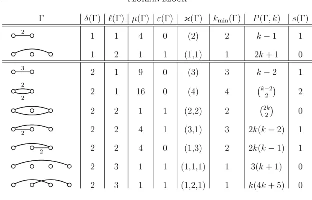
Definition 3.2. A template Γ is a directed graph (with possibly multiple edges) on vertices{0, . . . , l}, for l≥1, and edge weights w(e)∈Z>0, satisfying:
(1) Ifi→j is an edge then i < j.
(2) Every edgei→e i+ 1 has weight w(e)≥2. (No “short edges.”)
(3) For each vertex j, 1 ≤ j ≤ l −1, there is an edge “covering” it, i.e., there exists an edgei→k with i < j < k.
Every template Γ comes with some numerical data associated with it. Its length l(Γ) is the number of vertices minus 1. The product of squares of the edge weights is its multiplicity µ(Γ). Its cogenus δ(Γ) is
δ(Γ) =X i→ej (j−i)w(e)−1 .
For 1 ≤ j ≤ l(Γ) let κj = κj(Γ) denote the sum of the weights of edges i → k
with i < j ≤k and define
kmin(Γ) = max
Γ δ(Γ) `(Γ) µ(Γ) ε(Γ) κ(Γ) kmin(Γ) P(Γ, k) s(Γ) d 2 d 1 1 4 0 (2) 2 k−1 1 d d d 1 2 1 1 (1,1) 1 2k+ 1 0 d 3 d 2 1 9 0 (3) 3 k−2 1 d 2 d 2 2 1 16 0 (4) 4 k−2 2 2 d d d 2 2 1 1 (2,2) 2 2k 2 0 d d d 2 2 2 4 1 (3,1) 3 2k(k−2) 1 d d d 2 2 2 4 0 (1,3) 2 2k(k−1) 1 d d d d 2 3 1 1 (1,1,1) 1 3(k+ 1) 0 d d d d 2 3 1 1 (1,2,1) 1 k(4k+ 5) 0
Figure 1. The templates with δ(Γ)≤2.
This makeskmin(Γ) the smallest positive integer k such that Γ can appear in a floor diagram on {1,2, . . .}with left-most vertex k. Lastly, set
ε(Γ) =
1 if all edges arriving at l have weight 1,
0 otherwise.
Figure 1 (Figure 10 taken from [7]) lists all templates Γ with δ(Γ)≤2.
A labeled floor diagram D with d vertices decomposes into an ordered collection (Γ1, . . . ,Γm) of templates as follows: First, add an additional vertexd+ 1 (> d) to D
along with, for every vertexjofD, 1−div(j) new edges of weight 1 fromj to the new vertexd+ 1. The resulting floor diagramD0 has divergence 1 at every vertex coming
from D. Now remove all short edges fromD0, that is, all edges of weight 1 between
consecutive vertices. The result is an ordered collection of templates (Γ1, . . . ,Γm),
listed left to right, and it is not hard to see that P
δ(Γi) = δ(D). This process is
reversible once we record the smallest vertexkiof each template Γi(see Example 3.3). Example 3.3. An example of the decomposition of a labeled floor diagram into templates is illustrated below. Here, k1 = 2 andk2 = 4.
e e 2 e e e - - -j * 3
-l
D = e e 2 e e e e - - -j * 3 - -j *l
D0 = e e 2 e e e e - 3 -(Γ1,Γ2) =To each template Γ we associate a polynomial that records the number of “mark-ings of Γ:” For k ∈ Z>0 let Γ(k) denote the graph obtained from Γ by first adding k+i−1−κi short edges connectingi−1 to i, for 1≤i≤l(Γ), and then subdividing
each edge of the resulting graph by introducing one new vertex for each edge. By [7, Lemma 5.6] the number of linear extensions (up to equivalence) of the vertex poset of the graph Γ(k) extending the vertex order of Γ is a polynomial ink, if k ≥kmin(Γ),
which we denote by P(Γ, k) (see Figure 1). The number of markings of a labeled floor diagram D decomposing into templates (Γ1, . . . ,Γm) is then
ν(D) =
m
Y
i=1
P(Γi, ki),
where ki is the smallest vertex of Γi in D. The algorithm is based on
Theorem 3.4 ([7], (5.13)). The Severi degree Nd,δ, for d, δ ≥ 1, is given by the template decomposition formula
(3.1) X (Γ1,...,Γm) m Y i=1 µ(Γi) d−l(Γm)+ε(Γm) X km=kmin(Γm) P(Γm, km)· · · k2−l(Γ1) X k1=kmin(Γ1) P(Γ1, k1),
where the first sum is over all ordered collections of templates (Γ1, . . . ,Γm), for all m ≥ 1, with Pm
i=1δ(Γi) = δ, and the sums indexed by ki, for 1 ≤ i < m, are over kmin(Γi)≤ki ≤ki+1−l(Γi),
Expression (3.1) can be evaluated symbolically, using the following two lemmata. The first is Faulhaber’s formula [10] from 1631 for discrete integration of polyno-mials. The second treats lower limits of iterated discrete integrals and its proof is straightforward. HereBj denotes thejth Bernoulli number with the convention that B1 = +12.
Lemma 3.5 ([10]). Let f(k) = Pd
i=0cik
i be a polynomial in k. Then, for n≥0,
(3.2) F(n)def= n X k=0 f(k) = d X s=0 cs s+ 1 s X j=0 s+ 1 j Bjns+1−j. In particular, deg(F) = deg(f) + 1.
Lemma 3.6. Let f(k1) and g(k2) be polynomials in k1 and k2, respectively, and let a1, b1, a2, b2 ∈ Z≥0. Furthermore, let F(k2) = Pk2
−b1
k1=a1f(k1) be a discrete
anti-derivative of f(k1), where k2 ≥a1+b1. Then, for n≥max(a1+b1+b2, a2+b2), n−b2 X k2=a2 g(k2) k2−b1 X k1=a1 f(k1) = n−b2 X k2=max(a1+b1,a2) g(k2)F(k2).
Example 3.7. An illustration of Lemma 3.6 is the following iterated discrete inte-gral: n X k2=1 k2−2 X k1=1 1 = n X k2=1 k2−2 if k2 ≥2 0 if k2 = 1 = n X k2=3 k2−2.
Data: The cogenus δ.
Result: The node polynomial Nδ(d). begin
Generate all templates Γ withδ(Γ)≤δ;
Nδ(d)←0;
forall the ordered collections of templates Γ = (Γ˜ 1, . . . ,Γm) with
Pm i=1δ(Γi) = δ do i←1; Q1 ←1; while i≤m do ai ←
max kmin(Γi), kmin(Γi−1)+l(Γi−1), . . . , kmin(Γ1)+l(Γ1)+· · ·+l(Γi−1)
; end while i≤m−1 do Qi+1(ki+1)←P ki+1−l(Γi) ki=ai P(Γi, ki)Qi(ki); i←i+ 1; end Q˜Γ(d)←Pd−l(Γm)+ε(Γm) km=am P(Γm, km)Qm(km); Q˜Γ(d)←Qm i=1µ(Γi)·Q ˜ Γ(d); Nδ(d)←Nδ(d) +Q ˜ Γ(d); end end
Algorithm 1: Algorithm to compute node polynomials.
Using these results Algorithm 1 computes node polynomialsNδ(d) for an arbitrary
number of nodes δ. The first step, the template generation, is explained later in this section.
Proof of Correctness of Algorithm 1. The algorithm is a direct implementation of Theorem 3.4. The m-fold discrete integral is evaluated symbolically, one sum at a time, using Faulhaber’s formula (Lemma 3.5). The lower limit ai of the ith sum is
given by an iterated application of Lemma 3.6.
As Algorithm 1 is stated its termination in reasonable time is hopeless for δ ≥8 or 9. The novelty of this section, together with an explicit formulation, is how to implement the algorithm efficiently. This is explained in Remark 3.8.
Remark 3.8. The running time of the algorithm can be improved vastly as follows: As the limits of summation in (3.1) only depend on kmin(Γi), l(Γi) and ε(Γm), we
can replace the template polynomials P(Γi, ki) by PP(Γi, ki), where the sum is
over all templates Γi with prescribed (kmin, l, ε). After this transformation the first
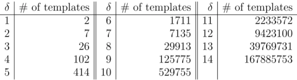
sum in (3.1) is over all combinations of those tuples. This reduces the computation drastically as, for example, the 167885753 templates of cogenus 14 make up only 343 equivalence classes. Also, in (3.1) we can distribute the template multiplicities
µ(Γi) and replace P(Γi, ki) by µ(Γi)P(Γi, ki) and thereby eliminate
Q
µ(Γi).
An-other speed-up is to compute all discrete integrals of monomials using Lemma 3.5 in advance.
The generation of the templates is the bottleneck of the algorithm. Their number grows rapidly with δ as can be seen from Figure 3. However, their generation can be parallelized easily (see below).
Algorithm 1 has been implemented in Maple. Computing N14(d) on a machine
with two quad-core Intel(R) Xeon(R) CPU L5420 @ 2.50GHz, 6144 KB cache, and 24 GB RAM took about 70 days.
Remark 3.9. Using the combinatorial framework of floor diagrams one can show that alsorelative Severi degrees(i.e., the degrees ofgeneralized Severi varieties, see [5, 14]) are polynomial and given by “relative node polynomials” [1, Theorem 1.1]. This suggests the existence of a generalization of G¨ottsche’s Conjecture [8, Conjecture 2.1] and the G¨ottsche-Yau-Zaslow formula [8, Conjecture 2.1]. Thus, the combinatorics of floor diagrams lead to new conjectures although the techniques and results seem to be out of reach at this time.
Remark 3.10. We can use Algorithm 1 to compute the values of the Severi degrees
Nd,δ for prescribed values of d and δ. After we specify a degree d and a number of nodes δ all sums in our algorithm become finite and can be evaluated numerically. See Appendix B for all values ofNd,δ for 0≤δ≤14 and 1≤d≤13.
Proof of Proposition 1.4. For 1 ≤δ ≤14 we observe, using the data in Appendices A and B, thatNδ(d) =Nd,δ for alld0(δ)≤d < δ, whered0(δ) =
δ
2
+ 1 is G¨ottsche’s threshold. Furthermore, Nδ(d0(δ)−1)6=Nd0(δ)−1,δ for all 3≤δ≤14. Template Generation. To compute a list of all templates of a given cogenus one can proceed as follows. First, we need some terminology and notation. An edge
i →j of a template is said to have length j −i. A template Γ is of type α = (αij), i, j ∈ Z>0, if Γ has αij edges of length i and weight j. Every type α satisfies, by
definition of cogenus of a template,
(3.3) X
i,j≥1
αij(i·j−1) = δ(Γ).
Note that α11= 0 as short edges are not allowed in templates. The number of types
constituting a given cogenus δ is finite.
We can generate all templates of typeαusing a branch-and-bound algorithm which slides edges in a suitable order. Let Γ0 be the unique template of type α with all
edges emerging from vertex 0. Fix a linear order on the set of edges of type α. For example, if α = 0 1 2 0 , we could choose: d d 2 - d d d
-<
d d d-<
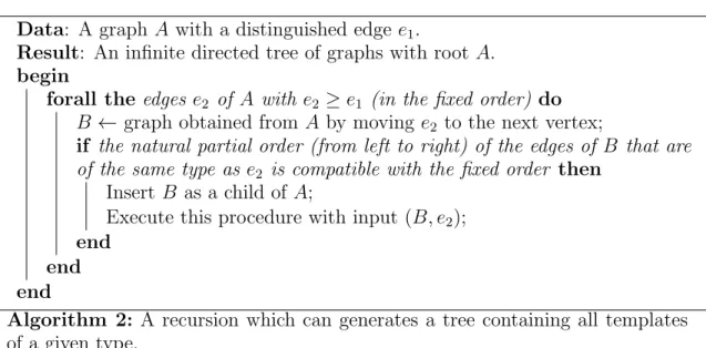
.Data: A graphA with a distinguished edge e1.
Result: An infinite directed tree of graphs with rootA.
begin
forall the edges e2 of A with e2 ≥e1 (in the fixed order) do B ← graph obtained fromA by moving e2 to the next vertex;
if the natural partial order (from left to right) of the edges of B that are of the same type as e2 is compatible with the fixed order then
Insert B as a child of A;
Execute this procedure with input (B, e2); end
end end
Algorithm 2: A recursion which can generates a tree containing all templates of a given type.
Algorithm 2 applied to the pair (Γ0, e0), wheree0is the smallest edge of Γ0, creates
an infinite directed tree with root Γ0 all of whose vertices correspond to different
graphs. Eliminate a branch if either
(1) no edge of the root of the branch starts at vertex 1, or
(2) condition (3) in Definition 3.2 is impossible to satisfy for graphs further down the tree.
See Figure 3 for an illustration for α = 0 1 2 0 . b b b 2 -Γ0 = {{wwwwww www ## G G G G G G G G G b b b b 2 -{{wwwwww www b b b 2 -{{wwwwww www b b b b b 2 P P P P P PP b-2 b b b P P P P P PP b b-2 b b -{{wwwwww www b b b b 2 -- ! {{wwwwww www b b b b b 2 P P P P P PP b b b-2 b b b b b 2 P P P P P PP b b b b b 2 P P P P PP P
Figure 2. Branch-and-bound tree for α=
0 1 2 0
A complete, non-redundant list of all templates of type α is then given by all remaining graphs which satisfy condition (3) of Definition 3.2 as every template can be obtained in a unique way from Γ0 by shifting edges in an order that is compatible
with the order fixed earlier. Note that it can happen that a non-template graph precedes a template within a branch. For an example see the graph in brackets in Figure 3. Template generation for different types can be executed in parallel. The number of templates, for δ≤14, is given in Figure 3.
δ # of templates δ # of templates δ # of templates
1 2 6 1711 11 2233572
2 7 7 7135 12 9423100
3 26 8 29913 13 39769731
4 102 9 125775 14 167885753
5 414 10 529755
Figure 3. The number of templates with cogenus δ ≤14.
4. Threshold Values
S. Fomin and G. Mikhalkin [7, Theorem 5.1] proved polynomiality of the Severi degrees Nd,δ in d, for fixed δ, provided d is sufficiently large. More precisely, they showed that Nδ(d) = Nd,δ for d ≥ 2δ. In this section we show that their threshold
can be improved to d≥δ (Theorem 1.3).
We need the following elementary observation about robustness of discrete anti-derivatives of polynomials whose continuous counterpart is the well known fact that
Ra−s−1
a−1 f(x)dx= 0 iff(x) = 0 on the interval (a−s−1, a−1). Lemma 4.1. For a polynomial f(k)and a∈Z>0 let F(n) =
Pn
k=af(k) be the poly-nomial in n uniquely determined by large enough values of n. (F(n)is a polynomial by Lemma 3.5.) If we havef(a−1) =· · ·=f(a−s) = 0for some0≤s < a(this con-dition is vacuous fors = 0) then it also holds thatF(a−1) = · · ·=F(a−s−1) = 0. In particular, Pn
k=af(k) is a polynomial in n, for n≥a−s−1.
Even for s= 0 the lemma is non-trivial as, in general,F(a−2)6= 0.
Proof. Let G(n) be the polynomial in n defined via G(n) =Pn
k=0f(k) for large n.
ThenF(n) =G(n)−Pa−1
k=0f(k) for all n∈Z≥0. In particular, for any 0 ≤i≤s, we
haveF(a−i−1) = G(a−i−1)−Pa−1
k=0f(k) = G(a−i−1)−
Pa−i−1
k=0 f(k) = 0.
Recall that for a template Γ, we defined kmin =kmin(Γ) to be the smallest k ≥1 such that k+j −1≥κj(Γ) for all 1≤ j ≤l(Γ). Let j0 be the smallest j for which
equality is attained (it is easy to see that equality is attained for some j). Define
s(Γ) to be the number of edges of Γ fromj0−1 toj0 (of any weight). See Figure 1 for
some examples. The following lemma shows that the template polynomials P(Γ, k) satisfy the condition of Lemma 4.1.
Lemma 4.2. With the notation from above it holds that
P(Γ, kmin−1) =P(Γ, kmin−2) = · · ·=P(Γ, kmin−s(Γ)) = 0.
Proof. Recall from Section 3 that, fork ≥kmin(Γ), the polynomialP(Γ, k) records the number of linear extension (up to equivalence) of some poset Γ(k) which is obtained
from Γ by first adding k +j −1−κj(Γ) “short edges” connecting j −1 to j, for
1≤j ≤l(Γ), and then subdividing each edge of the resulting graph by introducing a new vertex for each edge.
Using the notation from the last paragraph notice thatkmin+j0−1 =κj0(Γ), and
thus Γ(k) has k−kmin “short edges” between j0−1 and j0. Every linear extension of
Γ(k) can be obtained by first linearly ordering the midpoints of these k−kmin “short
edges” and the midpoints of the s(Γ) many edges of Γ connecting j0 − 1 and j0
before completing the linear order to all vertices of Γ(k). Therefore, the polynomial
(k−kmin+ 1)· · ·(k−kmin+s(Γ)) dividesP(Γ, k).
Before we can prove Theorem 1.3 we need a last technical lemma.
Lemma 4.3. Using the notation from above we have, for each template Γ, kmin(Γ)−s(Γ) +l(Γ)−ε(Γ)≤δ(Γ) + 1.
Proof. As before, letj0 be the smallest j in{1, . . . , l(Γ)} with kmin+j−1 =κj(Γ).
It suffices to show that κj0(Γ)−j0−s(Γ) +l(Γ)−ε(Γ)≤δ(Γ).
Let Γ0 be the template obtained from Γ by removing all edges i → k with either
k < j0 ori ≥ j0. It is easy to see that l(Γ)−ε(Γ)−(l(Γ0)−ε(Γ0)) ≤δ(Γ)−δ(Γ0).
Thus, we can assume without loss of generality that all edges i → k of Γ satisfy
i < j0 ≤k. Therefore, asκj0(Γ) =
P
edgeseof Γwt(e) it suffices to show that
(4.1) l(Γ)−ε(Γ)≤ X
edgeseof Γ
h
wt(e)(len(e)−1)−1i+s(Γ) +j0,
where len(e) is the length of an edge e. The contribution of the s(Γ) edges of Γ between j0−1 and j0 to the sum is −s(Γ), thus the right-hand-side of (4.1) equals
(4.2) X hwt(e)(len(e)−1)−1i+j0
with the sum now running over all edges of Γ of length at least 2. If there are no such edges, then l(Γ) = 1 and we are done. Otherwise, ifε(Γ) = 1, expression (4.2) equals P
(len(e)−2) +j0, which is ≥l(Γ)−2 +j0 or≥l(Γ)−3 +j0 if j0 ∈ {1, l(Γ)}
or 1< j0 < l(Γ), respectively (by considering only edges adjacent to vertices 0 and l(Γ) of Γ). In either case the result follows.
If ε(Γ) = 0 then expression (4.2) is ≥ l(Γ) + (l(Γ)−3 +j0) or ≥l(Γ)−2 +j0 if j0 ∈ {1, l(Γ)} or 1< j0 < l(Γ), respectively. This completes the proof.
Proof of Theorem 1.3. By Lemma 3.6 and repeated application of Lemmata 4.1 and 4.2 it suffices to show that d≥δ simultaneously implies
d≥l(Γm)−ε(Γm) +kmin(Γm)−s(Γm)−1, d≥l(Γm)−ε(Γm) +l(Γm−1) +kmin(Γm−1)−s(Γm−1)−2, .. . d≥l(Γm)−ε(Γm) +l(Γm−1) +· · ·+l(Γ1) +kmin(Γ1)−s(Γ1)−m, (4.3)
for all collections of templates (Γ1, . . . ,Γm) with Pmi=1δ(Γi) =δ.
The first inequality is a direct consequence of Lemma 4.3. For the other inequali-ties, notice that l(Γ)−ε(Γ)≤δ(Γ) for all templates Γ, hence
l(Γm)−ε(Γm)−1≤δ(Γm)−1
and
l(Γi)−1≤δ(Γi), for 2≤i≤m−1.
By Lemma 4.3 we have
l(Γ1) +kmin(Γ1)−s(Γ1)−1≤δ(Γ1) + 1
asε(Γ1)≤1, and the right-hand-side of the last inequality of (4.3) is≤Pmi=1δ(Γi) =
δ≤d. The proof of the other inequalities is very similar.
5. Coefficients of Node Polynomials
The goal of this section is to present an algorithm for the computation of the coefficients of Nδ(d), for generalδ. The algorithm can be used to prove Theorem 1.2
and thereby confirm and extend a conjecture of P. Di Francesco and C. Itzykson in [6] where they conjectured the 7 terms ofNδ(d) of largest degree.
Our algorithm should be able to find formulas for arbitrarily many coefficients of
Nδ(d). We prove correctness of our algorithm in this section. The algorithm rests on
the polynomiality of solutions of certain polynomial difference equations (see (5.7)). First, we fix some notation building on terminology of Section 3. By Remark 3.8 we can replace the polynomialsP(Γ, k) in (3.1) by the productµ(Γ)P(Γ, k), thereby removing the productQ
µ(Γi) of the template multiplicities. In this section we write P∗(Γ, k) for µ(Γ)P(Γ, k). For integers i≥ 0 and a ≥0 let Mi(a) denote the matrix
of the linear map
(5.1) f(k)7→ X Γ:δ(Γ)=i n−l(Γ) X k=kmin(Γ) P∗(Γ, k)·f(k),
where f(k) = c0ka + c1ka−1 +· · ·, a polynomial of degree a, is mapped to the polynomial Mi(a)(f(k)) = d0na+i+1 +d1na+i +· · · in n. (By Lemma 3.5 and the
proof of Lemma 5.1 the image has degree a+i+ 1.) Hence Mi(a)c=d. Similarly,
define Mend
i (a) to be the matrix of the linear map
(5.2) f(k)7→ X Γ:δ(Γ)=i n−l(Γ)+ε(Γ) X k=kmin(Γ) P∗(Γ, k)·f(k).
Later we will consider square sub-matrices ofMi(a) andMiend(a) by restriction to
the first few rows and columns which will be denoted Mi(a) and Miend(a) as well.
Note that Mi(a) andMiend(a) are lower triangular. For example, fora large enough,
M1(a) = 6 a+2 0 0 0 0 · · · −5a+8 a+1 6 a+1 0 0 0 · · · 5 2a+ 3 − 5a+3 a 6 a 0 0 · · · −1 4(4a+ 1)a 5 2a+ 1 2 − 5a−2 a−1 6 a−1 0 · · · 1 40(13a 2−20a+ 7)a −a2+7 4a− 3 4 5 2a−2 − 5a−7 a−2 6 a−2 · · · .. . ... ... ... ... . .. .
Lemma 5.1. The first a+i rows ofMi(a)and Miend(a)are independent of the lower limits of summation in (5.1) and (5.2), respectively.
Proof. It is an easy consequence of the proof of [7, Lemma 5.7] that the polynomial
P∗(Γ, k) associated with a template Γ has degree ≤ δ(Γ). Equality is attained by the template Γ on vertices 0,1,2 with i edges connecting 0 and 2 (so δ(Γ) =i). As discrete integration of a polynomial increases the degree by 1 the polynomial on the
right-hand-side of (5.1) has degree 1 +i+a.
The basic idea of the algorithm is that templates with higher cogenera do not contribute to higher degree terms of the node polynomial. With this in mind we define, for each finite collection (Γ1, . . . ,Γm) of templates, its type τ = (τ2, τ3, . . .),
whereτi is the number of templates in (Γ1, . . . ,Γm) with cogenus equal toi, fori≥2.
Note that we do not record the number of templates with cogenus equal to 1. To collect the contributions of all collections of templates with a given type τ, let τ = (τ2, τ3, . . .) and fix δ ≥ P
j≥2τj (so that there exist template collections
(Γ1, . . . ,Γm) of type τ with
P
δ(Γj) = δ). We define two (column) vectors Cτ(δ)
and Cend
τ (δ) as the coefficient vectors, listed in decreasing order, of the polynomials
(5.3) X (Γ1,...,Γm) n−l(Γm) X km=kmin(Γm) P∗(Γm, km)· · · k2−l(Γ1) X k1=kmin(Γ1) P∗(Γ1, k1) and (5.4) X (Γ1,...,Γm) n−l(Γm)+ε(Γ) X km=kmin(Γm) P∗(Γm, km) km−l(Γm−1) X km−1=kmin(Γm−1) · · · k2−l(Γ1) X k1=kmin(Γ1) P∗(Γ1, k1)
in the indeterminaten, where the respective first sums are over all ordered collections of templates of type τ.
It might look like Cτ(δ) is a product of some matrices Mi(a) applied to the
poly-nomial 1. However, this is not the case. For example, note that
C(0,0,...)(2) = 9 2 −34 88 −179 2 30 0 .. . 6 = 9 2 −34 88 −179 2 27 0 .. . =M1(2)·M1(0)· 1 0 0 0 0 0 .. . .
This is because, when iterated discrete integrals are evaluated symbolically, the lower limits of integration of the outer sums can change depending on the limits of the inner sums (cf. Lemma 3.6). This observation makes it necessary to compute initial values for recursions (described later) up to a large enough δ.
Before we can state the main recursion we need two more notations. For a type
τ = (τ2, τ3, . . .) and i ≥ 2 with τi > 0 define a new type τ↓i via (τ↓i)i =τi−1 and
(τ↓i)j = τj for j 6= i. Furthermore, let def(τ) = Pj≥2(j −1)τj be the defect of τ.
The following lemma justifies this terminology.
Lemma 5.2. The polynomials (5.3) and (5.4) are of degree 2δ−def(τ). Proof. Let (Γ1, . . . ,Γm) be a collection of templates with
Pm
i=1δ(Γi) =δ and type τ.
Then, by applying the argument in the proof of Lemma 5.1 to each Γi, the
polyno-mials (5.3) and (5.4) have degree δ+m. The result follows as
δ−def(τ) = m X i=1 δ(Γi)− X j≥2 (j −1)τj = m X i=1 δ(Γi)− X j≥2 X i:δ(Γi)=τj δ(Γi) −τj = #{i:δ(Γi) = 1}+ X j≥2 τj =m.
The last lemma makes precise which collections of templates contribute to which coefficients of Nδ(d). Namely, the first N coefficients of Nδ(d) of largest degree
depend only on collections of templates with types τ such that def(τ) < N. The following recursion is the heart of the algorithm.
Proposition 5.3. For every type τ and integer δ large enough, it holds that Cτ(δ) = X i:τi6=0 Mi 2δ−i−1−def(τ) Cτ↓i(δ−i) +M1 2δ−2−def(τ) Cτ(δ−1). (5.5)
More precisely, if we restrict all matrices Mi to be square of size N−def(τ) and all Cτ to be vectors of length N −def(τ), then recursion (5.5) holds for
δ ≥max N + 1 2 ,X j≥2 jτj ! .
Proof. The coefficient vector Cτ(δ) is defined by a sum that runs over all collections
of templates (Γ1, . . . ,Γm) of type τ (see (5.3)). Partition the set of such collections
by puttingδ(Γm) = 1, orδ(Γm) = 2, and so forth. This partitioning splits expression
(5.3) exactly as in (5.5).
A summand can be written as a product of some matrixMi and some vectorCτ↓i
if δ is large enough, namely ifMi does not depend on the lower limits in (5.3). If we
can factor then the polynomials (5.3) defining Cτ↓i(δ−i) andCτ(δ−1) have degrees
2(δ−i)−def(τ↓i) = 2δ−2i−def(τ) + (i−1) = 2δ−i−1−def(τ)
by Lemma 5.2 and, similarly, 2δ−2−def(τ), respectively. By Lemma 5.1, if the matrix Mi(2δ−i−1−def(τ)) is of size N−def(τ), then it does not depend on the
lower limits if and only if δ ≥ N+1
2 . In order for Cτ(δ) to be defined (and the above
identity to be meaningful) we need to impose δ≥P
j≥2jτj.
Remark 5.4. Later, when we formulate the algorithm, we need to solve recursion (5.5) together with an initial condition in order to obtain an explicit formula for the first N −def(τ) entries of Cτ(δ). It suffices to take
(5.6) δ0(τ) def = max N −1 2 ,X j≥2 jτj !
as for any δ > δ0(τ) the vector Cτ(δ) of length N −def(τ) can be written in terms
of matrices Mi and vectors Cτ0(δ0) for various types τ0 and integers δ0 < δ.
We propose Algorithm 3 for the computation of the coefficients of the node poly-nomial Nδ(d). We explain how to solve recursion (5.5) below.
Proof of Correctness of Algorithm 3. Proposition 5.3 guarantees thatCτ(δ) is uniquely
determined by recursion (5.3). By a similar argument as in the proof of Proposi-tion 5.3 we see that Cend
τ (δ) is given by the formula in Algorithm 3. By Lemma 5.2
all contributions of template collections of type τ to the node polynomial Nδ(d) are
in degree 2δ−def(τ) or less. Hence, after shifting Cend
τ (δ) by def(τ), their sum is
the coefficient vector of Nδ(d).
To solve recursion (5.5) for a type τ we make use of the following (conjectural) structure about Cτ(δ) which has been verified for all types τ with def(τ)≤ 8. This
refines an observation of L. G¨ottsche [8, Remark 4.2 (2)] about the first 28 (conjec-tural) coefficients of the node polynomial Nδ(d).
Conjecture 5.5. All entries of Cτ(δ) are of the form 3 δ
Data: A positive integer N.
Result: The coefficient vectorC of the firstN coefficients of Nδ(d). begin
Compute all templates Γ withδ(Γ)≤N;
forall the types τ with def(τ)< N do
Compute initial values Cτ(δ0(τ)) using (5.3), with δ0(τ) as in (5.6);
Solve recursion (5.5) for first N −def(τ) coordinates of Cτ(δ);
Set Cτend(δ)← X i:τi6=0 Miend 2δ−i−1−def(τ)Cτ↓i(δ−i) +M1end 2δ−2−def(τ)Cτ(δ−1); end C ←0;
forall the types τ with def(τ)< N do
Shift the entries of Cτend(δ) down by def(τ);
C ←C+ shifted Cend τ (δ); end
end
Algorithm 3: Computation of the leading coefficients of the node polynomial. Now, to solve recursion (5.5), we first extend the natural partial order on the types
τ given by|τ|=P
j≥2τj to a linear order with smallest element τ = (0,0, . . .). For
example, forN = 4, we could take
(0,0,0)<(1,0,0)<(0,1,0)<(0,0,1)<(1,1,0)<(2,0,0)<(3,0,0).
Then solve recursion (5.5) for eachτ, in increasing order, using the lowertriangularity of the matrices Mi. For example, to compute the second entry 3
δ
δ!p(δ) of C1,1(δ)
(assuming Conjecture 5.5), where p(δ) is a polynomial in δ, we need to solve
C1,1(δ) = M1(2δ−5)C1,1(δ−1) +M2(2δ−6)C0,1(δ−2) +M3(2δ−7)C1,0(δ−3), or, explicitly, ∗ 3δ δ!p(δ) .. . = ∗ 0 0 ∗ ∗ 0 .. . ... . .. ∗ 3δ−1 (δ−1)!p(δ−1) .. . + ∗ 0 0 ∗ ∗ 0 .. . ... . .. ∗ ∗ .. . + ∗ 0 0 ∗ ∗ 0 .. . ... . .. ∗ ∗ .. . .
The∗-entries in the vectorsC0,1 andC1,0 are known by a previous computation. The
∗-entries inM1,M2 and M3 are given by (5.3). The proof of Lemma 5.1 implies that
all denominators ofMi(a) in rowjarea+i−j+2 or 1 (after cancellation). To compute p(δ), or, more generally, the jth entry inCτ(δ), we first clear all denominators and
then solve the polynomial difference equation with initial conditions (2δ−def(τ)−j+ 1)3p(δ) = p(δ−1) +q(δ),
p(δ0(τ)) = Cτ(δ0(τ)),
whereq(δ) is a rather complicated polynomial depending on earlier calculations and
δ0(τ) is as in (5.6). One way to solve (5.7) is to bound the degree of the polynomial p(δ) and solve the corresponding linear system.
Note that a difference equation of the form (5.7) need not have a polynomial solution in general. Conjecture 5.5 is equivalent to all recursions (5.7) appearing in Algorithm 3 to have a polynomial solution.
As in Section 3 (Remark 3.8), Algorithm 3 can be improved significantly by sum-ming the template polynomialsP(Γ, k) for templates Γ with fixed kmin(Γ), l(Γ), ε(Γ) in advance. Algorithm 3 has been implemented in Maple. Once the templates are known the bottleneck of the algorithm is the initial value computation which, with an improved implementation, should be faster than the template enumeration. Hence we expect Algorithm 3 to compute the first 14 terms of Nδ(d) in reasonable time.
Appendix A. Node Polynomials for δ≤14
An explicit list of Nδ(d), for δ ≤ 14, is as below. These polynomials are given
implicitly in Theorem 3.1. For δ ≤ 8 this agrees with [9, Theorem 3.1]. For δ ≤14 this coincides with the conjectural (implicit) formulas of [8, Remark 2.5].
N0(d) = 1, N1(d) = 3(d−1)2, N2(d) = 3 2(d−1)(d−2)(3d 2−3d−11), N3(d) = 9 2d 6−27d5+9 2d 4+423 2 d 3−229d2−829 2 d+ 525, N4(d) = 27 8d 8−27d7+1809 4 d 5−642d4−2529d3+37881 8 d 2+18057 4 d−8865, N5(d) = 81 40d 10−81 4d 9−27 8 d 8+2349 4 d 7−1044d6−127071 20 d 5+128859 8 d 4+59097 2 d 3−3528381 40 d 2 −946929 20 d+ 153513, N6(d) = 81 80d 12−243 20d 11−81 20d 10+8667 16 d 9−9297 8 d 8−47727 5 d 7+2458629 80 d 6+3243249 40 d 5 −6577679 20 d 4−25387481 80 d 3+6352577 4 d 2+8290623 20 d−2699706, N7(d) = 243 560d 14−243 40d 13−243 80d 12+30861 80 d 11−38853 40 d 10−802143 80 d 9+3140127 80 d 8+18650493 140 d 7 −54903831 80 d 6−72723369 80 d 5+124680069 20 d 4+213537633 80 d 3−3949576431 140 d 2−188754021 140 d + 48016791, N8(d) = 729 4480d 16−729 280d 15−243 140d 14+35721 160 d 13−25839 40 d 12−320841 40 d 11+11847087 320 d 10 +170823033 1120 d 9−6685218 7 d 8−1758652263 1120 d 7+1102682031 80 d 6+59797545 8 d 5−510928080111 4480 d 4 −3283674393 1120 d 3+558215113803 1120 d 2−3722027733 56 d−861732459, N9(d) = 243 4480d 18−2187 2240d 17−729 896d 16+121743 1120 d 15−99549 280 d 14−824823 160 d 13+8776593 320 d 12+74122857 560 d 11 −2188424421 2240 d 10−132610923 70 d 9+11404136871 560 d 8+2852923401 224 d 7−3523392270287 13440 d 6 +4109675615 448 d 5+261844582229 128 d 4−2156232149611 3360 d 3−29528525065861 3360 d 2+438722045999 168 d + 15580950065,
N10(d) = 729 44800d 20− 729 2240d 19− 729 2240d 18+408969 8960 d 17−746253 4480 d 16−1932579 700 d 15+10649961 640 d 14 +205722099 2240 d 13−4375229931 5600 d 12−38815692777 22400 d 11+30958937073 1400 d 10+3413568339 224 d 9 −3624162885799 8960 d 8+134470136581 2800 d 7+27023302169081 5600 d 6−22514488581251 8960 d 5−811909836973903 22400 d 4 +253124357071961 11200 d 3+867510616107447 5600 d 2−2800250331071 40 d−283516631436, N11(d) = 2187 492800d 22− 2187 22400d 21− 729 6400d 20+150903 8960 d 19−303993 4480 d 18−56670273 44800 d 17+47717667 5600 d 16 +295979589 5600 d 15−11410430877 22400 d 14−4051907631 3200 d 13+52491198663 2800 d 12+3418059518271 246400 d 11 −20587006282467 44800 d 10+2236636275459 22400 d 9+49175916627959 6400 d 8−1464110674563 256 d 7 −1946239824069277 22400 d 6+3767687640687823 44800 d 5+14264414890838423 22400 d 4−940418544772283 1600 d 3 −168280746183263029 61600 d 2+5073050867636909 3080 d+ 5187507215325, N12(d) = 2187 1971200d 24− 6561 246400d 23− 2187 61600d 22+496449 89600d 21−136809 5600 d 20−1618623 3200 d 19+674946837 179200 d 18 +2321658693 89600 d 17−893195181 3200 d 16−34334301951 44800 d 15+289702847403 22400 d 14+1245724147341 123200 d 13 −803786361621603 1971200 d 12+65497548165237 492800 d 11+16192295343681 1792 d 10−792669234543351 89600 d 9 −9506773589164709 67200 d 8+6296062244021929 33600 d 7+11029935159768347 7168 d 6−582428855393100577 268800 d 5 −5477484616918678589 492800 d 4+10067756533588172119 739200 d 3+4454424013895459501 92400 d 2 −111952943233924509 3080 d−95376705265437, N13(d) = 6561 25625600d 26− 6561 985600d 25− 19683 1971200d 24+1620567 985600d 23−88209 11200d 22−3212703 17920 d 21+262066023 179200 d 20 +494726373 44800 d 19−673360047 5120 d 18−35350103511 89600 d 17+20952637821 2800 d 16+3013479294723 492800 d 15 −580214902388013 1971200 d 14+1666286215401123 12812800 d 13+16384163286402207 1971200 d 12−909876952033137 89600 d 11 −7649416285706767 44800 d 10+25855007471662161 89600 d 9+65085797443981191 25600 d 8−108443195356282427 22400 d 7 −52991400162927629917 1971200 d 6+1976324604711031517 39424 d 5+13580753080243105219 70400 d 4 −73274705967431063281 246400 d 3−68173290776099374391 80080 d 2+2813974748454890667 3640 d+ 1761130218801033, N14(d) = 19683 358758400d 28− 19683 12812800d 27− 6561 2562560d 26+1751787 3942400d 25−4529277 1971200d 24−562059 9856 d 23 +398785599 788480 d 22+5214288411 1254400 d 21−4860008991 89600 d 20−63174295089 358400 d 19+332872084467 89600 d 18 +3103879378581 985600 d 17−4913807521304691 27596800 d 16+899178800016807 8968960 d 15+279086438050359453 44844800 d 14 −468967272863997483 51251200 d 13−318443311640108577 1971200 d 12+328351365725506869 985600 d 11 +1120586814080571923 358400 d 10−9448861028448843949 1254400 d 9−30880785216736406143 689920 d 8 +444525313669622586903 3942400 d 7+11429038221675466251 24640 d 6−269709254062572016617 246400 d 5 −74660630664748878665353 22422400 d 4+140531359469510983018159 22422400 d 3+16863931195154225977601 1121120 d 2 −64314454486825349085 4004 d−32644422296329680.
Appendix B. Small Severi degrees
Below we list the Severi degrees Nd,δ for 0≤ δ≤ 14 and 1≤d ≤13, which were
obtained by Algorithm 1 (also see Remark 3.10). Together with the node polynomials of Appendix A, this is a full description of all Severi degrees Nd,δ for δ ≤ 14, see
Theorem 1.3. The solid line segments indicate the polynomial threshold d∗(δ) of
Nd,δ. The dashed line segments illustrate the threshold of our Theorem 1.3. The Severi degreesNd,δ in italic agree with the Gromov-Witten invariantsNd,(d−1)(d−2)
2 −δ
, as ford≥δ+ 2, every plane degree d curve with δ nodes is irreducible.
d = 1 2 3 4 5 6 7 8 9 N d, 0 1 1 1 1 1 1 1 1 1 N d, 1 0 3 12 27 48 75 108 147 192 N d, 2 0 0 21 225 882 2370 5175 9891 17220 N d, 3 0 0 15 675 7915 41310 145383 40 4185 959115 N d, 4 0 0 0 666 36975 437517 2667375 11225145 37206936 N d, 5 0 0 0 378 90027 2931831 33720354 224710119 1068797961 N d, 6 0 0 0 105 109781 12597900 302280963 3356773532 23599 355991 N d, 7 0 0 0 0 65949 34602705 1950179922 38232604473 410453320698 N d, 8 0 0 0 0 26136 59809860 9108238023 336507128820 5717863228995 N d, 9 0 0 0 0 6930 63338881 30777542450 2307156326490 64541125393337 N d, 10 0 0 0 0 945 40047888 74808824094 12372036675723 595034126865816 N d, 11 0 0 0 0 0 15580020 129429708147 51941532804912 4504735527185481 N d, 12 0 0 0 0 0 4361721 157012934283 170460529136614 28096248183844557 N d, 13 0 0 0 0 0 918918 131024290671 435634878105750 144607321488666150 N d, 14 0 0 0 0 0 135135 73778495220 861893389007280 614331908473795659 d = 10 11 12 13 N d, 0 1 1 1 1 N d, 1 243 300 363 432 N d, 2 27972 43065 63525 90486 N d, 3 2029980 3939295 7139823 12245355 N d, 4 104285790 257991042 579308220 1203756165 N d, 5 4037126346 12886585236 36 161763120 91629 683271 N d, 6 122416062018 510681301550 1807308075111 5622246678741 N d, 7 2983927028787 16491272517465 74314664917722 285826689019395 N d, 8 59546865647151 442342707233400 2563893146687301 12282025653769635 N d, 9 985875034961260 9996104553443766 75318503191523715 452837863689428040 N d, 10 13675748317151382 192382226805469707 1905520429287295623 14494356139317787773 N d, 11 160116000544437849 3179784684983704875 41891284347920817345 406515611290526234685 N d, 12 1590895229889323034 45433391588342055421 806014803108359459265 10065752539264069119357 N d, 13 13467927464624076876 564072316378226731551 13651752114752769885861 221404946495996659008375 N d, 14 97415160821449934985 6109881487479049410675 204507963635254531972650 4348333391475310314325875
References
1. F. Block,Relative node polynomials for plane curves, Preprint, arXiv:1009.5063, 2010.
2. F. Block, A. Gathmann, and H. Markwig, Psi-floor diagrams and a Caporaso-Harris type recursion, Israel J. Math. (to appear) (2011).
3. E. Brugall´e and G. Mikhalkin, Enumeration of curves via floor diagrams, C. R. Math. Acad. Sci. Paris345(2007), no. 6, 329–334.
4. , Floor decompositions of tropical curves: the planar case, Proceedings of G¨okova Geometry-Topology Conference 2008, G¨okova Geometry/Topology Conference (GGT), G¨okova, 2009, pp. 64–90.
5. L. Caporaso and J. Harris, Counting plane curves of any genus, Invent. Math. 131 (1998), no. 2, 345–392.
6. P. Di Francesco and C. Itzykson,Quantum intersection rings, The moduli space of curves (Texel Island, 1994), Progr. Math., vol. 129, Birkh¨auser Boston, Boston, MA, 1995, pp. 81–148. 7. S. Fomin and G. Mikhalkin,Labeled floor diagrams for plane curves, J. Eur. Math. Soc. (JEMS)
12(2010), no. 6, 1453–1496.
8. L. G¨ottsche,A conjectural generating function for numbers of curves on surfaces, Comm. Math. Phys.196(1998), no. 3, 523–533.
9. S. Kleiman and R. Piene, Node polynomials for families: methods and applications, Math. Nachr.271(2004), 69–90.
10. D. Knuth,Johann Faulhaber and sums of powers, Math. Comp.61(1993), no. 203, 277–294. 11. G. Mikhalkin,Enumerative tropical geometry inR2, J. Amer. Math. Soc.18(2005), 313–377.
12. Y.-J. Tzeng,A proof of G¨ottsche-Yau-Zaslow formula, Preprint, arXiv:1009.5371, 2010. 13. I. Vainsencher, Enumeration ofn-fold tangent hyperplanes to a surface, J. Algebraic Geom.4
(1995), no. 3, 503–526.
14. R. Vakil,Counting curves on rational surfaces, Manuscripta Math.102(2000), no. 1, 53–84.
Department of Mathematics, University of Michigan, Ann Arbor, MI 48109, USA