Consistent ranking of multivariate volatility models

2009/2

■

Consistent ranking of multivariate volatility models

Sébastien Laurent, Jeroen V.K. Rombouts

and Francesco Violante

CORE

Voie du Roman Pays 34

B-1348 Louvain-la-Neuve, Belgium.

Tel (32 10) 47 43 04

Fax (32 10) 47 43 01

E-mail: [email protected]

http://www.uclouvain.be/en-44508.html

CORE DISCUSSION PAPER

2009/2

Consistent ranking of multivariate volatility models

Sébastien LAURENT

, Jeroen V.K. ROMBOUTS

and Francesco VIOLANTE

January 2009

Abstract

A large number of parameterizations have been proposed to model conditional variance dynamics in a multivariate framework. This paper examines the ranking of multivariate volatility models in terms of their ability to forecast out-of-sample conditional variance matrices. We investigate how sensitive the ranking is to alternative statistical loss functions which evaluate the distance between the true covariance matrix and its forecast. The evaluation of multivariate volatility models requires the use of a proxy for the unobservable volatility matrix which may shift the ranking of the models. Therefore, to preserve this ranking conditions with respect to the choice of the loss function have to be discussed. To do this, we extend the conditions defined in Hansen and Lunde (2006) to the multivariate framework. By invoking norm equivalence we are able to extend the class of loss functions that preserve the true ranking. In a simulation study, we sample data from a continuous time multivariate diffusion process to illustrate the sensitivity of the ranking to different choices of the loss functions and to the quality of the proxy. An application to three foreign exchange rates, where we compare the forecasting performance of 16 multivariate GARCH specifications, is provided.

Keywords: volatility, multivariate GARCH, matrix norm and loss function, norm equivalence.

JEL Classification: C10, C32, C51, C52, C53, G10

1_{Université de Namur, CeReFim, 5000 Namur, Belgium; Université catholique de Louvain, CORE,} B-1348 Louvain-la-Neuve, Belgium. E-mail: [email protected]

2 _{HEC Montréal, CIRANO, CIRPEE, Canada; Université catholique de Louvain, CORE, B-1348} Louvain-la-Neuve, Belgium.

3 _{Université de Namur, CeReFim, B-5000 Namur, Belgium; Université catholique de Louvain, CORE, B-1348}

Louvain-la-Neuve, Belgium. E-mail: [email protected]

Financial support from the CREF-HEC Montréal is gratefully acknowledged. We thank Luc Bauwens, Raouf Boucekkine and Lars Stentoft for helpful comments.

This paper presents research results of the Belgian Program on Interuniversity Poles of Attraction initiated by the Belgian State, Prime Minister's Office, Science Policy Programming. The scientific responsibility is assumed by the authors.

1

Introduction

A special feature of economic forecasting compared to general economic modeling is that we can measure a model’s performance by comparing its forecasts to the outcomes when they become available. Generally, several forecasting models are available for the same variable and models are compared through the computation of a loss function. Elliott and Timmermann (2008) provide an excellent survey on the state of the art of forecasting in economics. Details on volatility and correlation forecasting can be found in Andersen, Bollerslev, Christoffersen, and Diebold (2006).

The evaluation of the forecasting performance of volatility models raises an important problem. The variable of interest (i.e. volatility) being unobservable, the evaluation of the loss function has to rely on a proxy which may change the ordering. The impact on the ordering of the substitution of the true volatility by a proxy has been investigated in detail by Hansen and Lunde (2006). They provide conditions, for both the loss function and the volatility proxy, under which the approximated ranking (based on the proxy) is consistent for the true ranking (based on the true, but unobservable volatility).

Hansen and Lunde’s (2006) results have important implications for all testing procedures for superior predictive ability as in Diebold and Mariano (1995), West (1996), Clark and McCracken (2001), the reality check by White (2000), and the recent contributions of Hansen and Lunde (2005) with the superior predictive ability (SPA) test and Hansen, Lunde, and Nason (2003) with the Model Confidence Set test, among others. When the target variable is unobservable, an unfortunate choice of the loss function may deliver unintended results even when the testing procedure is formally valid.

In this paper, we extend findings of Hansen and Lunde (2006) to the multivariate framework. To forecast the conditional variance matrix of a portfolio of financial assets, we focus on multi-variate GARCH models (MGARCH) (see Bauwens, Laurent, and Rombouts (2006) for a survey), though the extension to other multivariate volatility models, like stochastic volatility and Markov switching models is straightforward. With respect to ranking models in the multivariate GARCH class, where conditional variance matrices are compared, little is known about the properties of the loss function.

We have four main contributions in this paper. First, we select a set of loss functions well suited to evaluate the differences in sequences of symetric positive definite matrices. We consider

six different loss functions based on matrix norms, namely the p-norm with p = 1 and p = 2

(the latter is known as the Frobenius norm), the spectral norm and their squared transformations. These loss functions are frequently used in practice.

Second, we derive conditions for consistent ranking for the multivariate case and we show that, though violating their conditions, a loss function might still lead to a consistent ranking if

norm equivalence can be invoked with respect to a consistent loss function. This result allows us to extend the requirements stated for univariate volatility models in Hansen and Lunde (2006) allowing loss functions that would be classified as inconsistent in the univariate case. For each of the loss functions considered in this paper we verify whether they satisfy the conditions to ensure a consistent ranking.

Third, through a comprehensive Monte Carlo simulation, we study the impact of the deteri-oration of the quality of the proxy on the ranking of MGARCH models with respect to different choices for the loss function. The true model is a multivariate diffusion from which we compute the integrated covariance as the true daily covariance. The MGARCH models are estimated on daily returns and used to compute 1-step ahead forecasts. The proxy of the daily covariance is Realized Covariance as defined in Andersen, Bollerslev, Diebold, and Labys (2003). The quality of this proxy is controlled through the level of aggregation of the simulated intraday data used to compute Realized Covariance. The main conclusion of this simulation is that inconsistent loss

functions are notper se inferior to consistent ones. When the quality of the proxy is sufficiently

good, consistency between the true and the approximated ranking can still be achieved. As the accuracy of the proxy deteriorates, the objective bias (i.e. the discrepancy between the true and the approximated ranking) becomes relevant and may affect the ordering between models.

Fourth, we illustrate our findings using three exchange rates (Euro, UK pound and Japanese yen against US dollar). We consider 16 MGARCH specifications which are frequently used in practice. The advantage of choosing a consistent loss function to evaluate model performances is striking. The ranking based on an inconsistent loss function, together with an uninformative proxy, is found to be severely biased. In fact, inferior models, that is models based on the RiskMetrics approach, emerge though it is unlikely that these are the best forecasting models. Overall, the set of 16 MGARCH models seem to produce conditional variance matrix predictions that are quite close.

The rest of the paper is organized as follows. Section 2 introduces the set of selected loss functions and revisits Hansen and Lunde’s (2006) conditions for consistent ranking. An additional condition, based on the notion of norm equivalence, is introduced. Section 3 provides a brief overview of several GARCH specification considered in this paper and thus constituting the fore-casting models set. In Section 4, we introduce realized covariance as a proxy for the unobserved conditional variance matrix. A detailed simulation study in Section 5 investigates the robustness of the ranking subject to consistent and inconsistent loss functions with respect to the level of accuracy of the proxy. The empirical application is presented in Section 6. Section 7 concludes.

2

Consistent ranking and distance metrics

As explained in Andersen, Bollerslev, Christoffersen, and Diebold (2006), the problem when com-paring and ranking forecasting performance of volatility models is that the true conditional vari-ance is unobservable so that a proxy for it is required. Let us define the true, or underlying, ordering between volatility models as the ranking implied by a loss function, evaluated with re-spect to the unobservable conditional covariance. The substitution of the latter by a proxy may introduce, because of its randomness, a ranking of volatility models that differs from the true one. Hansen and Lunde (2006) provide a theoretical framework for the analysis of the ordering of stochastic sequences and identify conditions that a loss function and the volatility proxy have to satisfy to deliver an ordering consistent with the true ranking when a proxy for the conditional co-variance is used. In this section, we discuss and extend these conditions to the case of multivariate volatility models.

We first fix some basic notations and make explicit what we mean by consistent ranking. For

N time series at timetwe haveM candidate models for the conditional variance matrix denoted

by H_it i = 1, . . . , M. Define L(·,·) an integrable loss function from RN×N _{→ R}+ _{such that}

L(Σt, Hit) is the loss function using the true but unobservable conditional variance matrix Σt.

SimilarlyL( ˆΣt, Hit) is the loss function using ˆΣt, a proxy of Σt. Consistency of ranking means

thatE(L(Σt, Hit))≥E(L(Σt, Hjt))⇔E(L( ˆΣt, Hit))≥E(L( ˆΣt, Hjt)) is true for alli=j.

2.1

Hansen and Lunde’s (2006) conditions for consistent ranking

Without loss of generality we can redefine the function L(., .) from the space of the N ×N

matrices toR+ as a scalar valued function from RN(N+1)/2 →R+ of all unique elements of the

matrices Σt and Hit since these are covariance matrices and therefore symetric. Let us denote

σ_t = [σ_kj,t] =vech(Σ_t) and h_i,t = [h_kj,it] =vech(H_it) wherevech(.) is the operator that stacks

the lower triangular portion of a matrix into a vector. As developed by Hansen and Lunde (2006) for univariate volatility models, similar relevant sufficient conditions to achieve consistency of the ranking for multivariate models are:

(i) L(Σt, Hit) and L( ˆΣt, Hit) have the same parametric form ∀i so that uncertainty depends

only on ˆΣtandtis a filtration such that ΣtandHit aret−1 measurable.

(ii) ∂2L(Σt,Hit)

∂σkj,t∂σkj,t is finite and does not depend on hkj,it ∀k, j, and, ξt = (ˆσt−σt) is a vector

martingale difference sequence with respect tot.

To illustrate the validity of the above conditions, consider the second order Taylor expansion

ofL(Σt, Hit) around the true value Σt:

L( ˆΣ_t, H_it)∼=L(Σ_t, H_it) + ∂L(Σ_t, H_it) ∂σt (ˆσ_t−σ_t) +1 2 (ˆσ_t−σ_t)∂ 2_L(Σ t, Hit) ∂σt∂σt (ˆσ_t−σ_t) . (1)

Taking conditional expections with respect tot−1 we get E(L( ˆΣt, Hit)|t−1) =∼ E(L(Σt, Hit)|t−1) +1₂ E ξ_t∂ 2_L(Σ t, Hit) ∂σt∂σt ξt|t−1 . (2)

When condition (i) and (ii) are satisfied we have

(a) E((L(Σt, Hit))

ξt|t−1) = (L(Σt, Hit))

E(ξt|t−1) = 0 whenever ˆσt is conditionally

unbi-ased with respect toσt;

(b) ∂2_L(Σ t,Hit) ∂σt∂σt

=f(σ_t2, .) does not depend on modeli.

HenceE(L( ˆΣt, Hit)|t−1) andE(L(Σt, Hit)|t−1) induce the same ordering overi.

The discrepancy between the true and the approximated ordering which is likely to occur

whenever condition (ii) is violated, is defined as objective bias. The objective bias must not

be confused with the sampling error. While the latter tend to disappear asymptotically (i.e.

T−1Σ_tL( ˆΣ_t, H_it) →p E(L( ˆΣ_t, H_it))), the presence of the objective bias may induce the sample

evaluation to be inconsistent for the true one independently from the sample size.

To conclude, (2) implies that in order to achieve consistency of the approximated ranking, the

equivalence betweenE(L( ˆΣt, Hit)|t−1) andE(L(Σt, Hit)|t−1) is not required, but it is sufficient

that the discrepancy,

E

ξ_tf(σ_t2, .)ξt|t−1 is constant across models, thus not affecting the

ranking. Notice, that the last term on the right hand side of (2) depends on the variance of

the proxy. Hence, even if condition (ii) is violated, that is

∂2L(Σt,Hit)

∂σt∂σt

= f(σ2_t, hit), the more

accurate the proxy, the less likely the objective bias. That is,

E

ξ_tf(σ2_t, hit)ξt|t−1 , though

depending oni, becomes negligible, leaving the ranking unaffected.

2.2

Norm equivalence

When the loss function is defined in terms of a matrix norm on the space ofN×N positive definite

matrices, SN×N_{, that isL(Σ}

t, Hit) = . _a, a useful property of matrix norms, namely the norm

equivalence, can be invoked. Norm equivalence is defined as follows (see Golub and Van Loan,

1996 or Horn and Johnson, 1985 for details). For any two matrix norms . _a and . _b on a finite

dimensional space, norm equivalence is defined as

k A _a≤ A _b≤l A _a, (3)

for 0 < k < l < ∞and A ∈ SN×N_{. If two norms are equivalent then they introduce the same}

topology onSN×N_{. This property is preserved under functional transformations - e.g. f(.) and}

g(.) of the matrix norms . _a and . _b, provided f( . _a) and g( . _b) have the same degree of

homogeneity.

A loss function based on matrix norms that satisfies condition (i) but violates (ii) may still

an inconsistent loss function can be established. In this case, the inconsistent loss function can

introduce the same ordering as the consistent one. This allows for the additional condition (iii)

which can be stated as follows.

(iii) Given a consistent loss functionLa(Σt, Hit) and another loss functionLb(Σt, Hit): kLa(Σt, Hit)≤

Lb(Σt, Hit)≤lLa(Σt, Hit) holds for 0< k < l <∞.

If (i) and (iii) holds forLb(Σt, Hit) then it is equivalent to the consistent loss functionLa(Σt, Hit)

and thus induces the same ordering.

The next section focuses on two families of loss functions which have been widely used in the

literature: thep-norm, the eigenvalue norm, and we also consider their square transformation. It

should be noted that while the p-norm and the Eigenvalue norm are valid norms, their squared versions are not since, though sharing most of the properties of matrix norms, they violate the homogeneity assumption, as they are homogeneous of degree two.

2.3

P-norm loss function

Thep-norm between two matrices (Σ_tandH_it) is defined as thepth_{-root of the sum of element-wise}

differences to the powerp, i.e.

L(Σ_t, H_it)_p= ⎛ ⎝ 1≤k,j≤N |σ_kj,t−h_kj,it|p ⎞ ⎠ 1/p . (4)

When p = 2 this norm is known as the Frobenius norm, while L(Σt, Hit)22 denotes its square

transformation. It is easy to show that, while the Frobenius norm does not satisfy condition

(ii), its squared version does, provided that ˆΣt is conditionally unbiased for Σt, that is when

E(ˆσ_kj,t2 |t−1) = σkj,t2 . In this paper, we consider also p = 1 (sum of absolute element-wise

differences) and its squareL(Σ_t, H_it)2₁. Thep-norm withp= 1 (and its square) violates condition

(ii) because it is not differentiable. However, we can show thatL(Σ_t, H_it)2₁satisfies condition (iii)

with respect to L(Σ_t, H_it)2₂ because of the following inequalities:

L(Σt, Hit)22≤L(Σt, Hit)21≤N2L(Σt, Hit)22, (5)

which comes directly from the norm equivalence betweenL(Σt, Hit)2andL(Σt, Hit)1. We illustrate

the proof in the bivariate case (N = 2). Letakj,t= (σkj,t−hkj,it)∀k, j= 1,2, so that

L(Σ_t, H_it)2₂ = k,j=1,2 a2_kj,t (6) L(Σ_t, H_it)2₁ = ⎡ ⎣ k,j=1,2 |a_kj,t| ⎤ ⎦ 2 (7) = k,j=1,2 a2_kj,t+ 2|a_12,t|2+ 2|a_11,t||a_22,t|+ 4|a_11,t||a_12,t|+ 4|a_12,t||a_22,t| (8)

≥ L(Σt, Hit)22, (9)

since for any two positive scalarsa_kj and a_lm, 2a_kja_lm≤a2_kj+a2_lm. We also have that

L(Σt, Hit)21≤4

k,j=1,2

a2_kj,t= 4L(Σt, Hit)22, (10)

which proves the result in (5). Using similar arguments for the p-norm with p= 1 we have

L(Σ_t, H_it)₂≤L(Σ_t, H_it)₁≤N L(Σ_t, H_it)₂. (11)

But in this case, since both L(Σt, Hit)1 and N L(Σt, Hit)2 do not satisfy condition (ii), though

equivalent, condition (iii) cannot be applied because condition (iii) is violated.

2.4

Eigenvalue loss function

The eigenvalue norm, also called spectral norm, is widely used in principal component analysis.

It is defined as the square root of the largest eigenvalue of the matrix (Σt−Hit)2 and denoted

by L(Σ_t, H_it)_E = λ_max(Σ_t, H_it). As before, we also consider its square transformation, i.e.

L(Σ_t, H_it)2_E = λ_max(Σ_t, H_it). As an illustration, the square of the eigenvalue norm becomes in

the bivariate case

L(Σt, Hit)2E = λmax[(Σt−Hit)2] (12) = 1 2f(σ11,t, σ12,t, σ22,t, hij,t) + 1 2 g(σ₁₁,t, σ12,t, σ22,t, hij,t), (13) where

f(σ₁₁,t, σ12,t, σ22,t, hkj,it) = (σ11,t−h11,it)2+ 2(σ12,t−h12,it)2+ (σ22,t−h22,it)2 (14)

g(σ_11,t, σ_12,t, σ_22,t, h_kj,it) = (σ11,t−h11,it)2−(σ22,t−h22,it)2 2 +

4(σ12,t−h12,it)2[(σ11,t−h11,it) + (σ22,t−h22,it)]2

. (15)

The second derivative of the loss function with respect toσ_kj,t2 is

1 2 f_σ2 kj,t+g σ2 kj,t . (16) Since g_σ2 kj,t and g σ2

kj,t depend on hkj,t condition (ii) is violated. However, we can show that

condition (iii) is satisfied with respect to the square of the Frobenius norm which in turn is

consistent by condition (ii). We can rewrite the Frobenius norm as

L(Σ_t, H_it)2₂=T race[(Σ_t−H_it)2] = N

λ_i, (17)

whereλi are the postive eigenvalues of the matrix (Σt−Hit)2. Therefore, we have

L(Σ_t, H_it)2_E =λ_max ≤

N

L(Σt, Hit)2E =λmax ≥ λ¯=N−1

N

λi=N−1L(Σt, Hit)2, (19)

which proves the following equivalence:

N−1L(Σt, Hit)22≤L(Σt, Hit)2E≤L(Σt, Hit)22. (20)

Therefore, using this loss function yields a consistent ranking becauseL(Σt, Hit)22 does.

As explained in Section 2.3, if we consider the spectral norm itself (i.e. the square root of the

highest eigenvalue of the matrix (Σt−Hit)) then by norm equivalence it holds

N−1/2L(Σt, Hit)2≤L(Σt, Hit)E≤L(Σt, Hit)2. (21)

This confirmsL(Σt, Hit)E to be ranking inconsistent because condition (iii) is violated.

3

Forecasting models set

In this paper, we focus on the ranking of multivariate volatility models that belong to the

MGARCH class. Consider a N-dimensional discrete time vector stochastic process rt. Let

μt = E(rt|t−1) be the conditional mean vector and Hit = E(rtrt|t−1) the conditional

vari-ance matrix for specificationiso that we can write the model of interest as:

r_t = μ_t+H_it1/2z_t, (22)

whereH_it1/2is a (N×N) positive definite matrix andztis an idependent and identically distributed

random innovation vector withE(zt) = 0 andV ar(zt) =IN.

In the application, we consider 16 specifications for Hit which are frequently used in

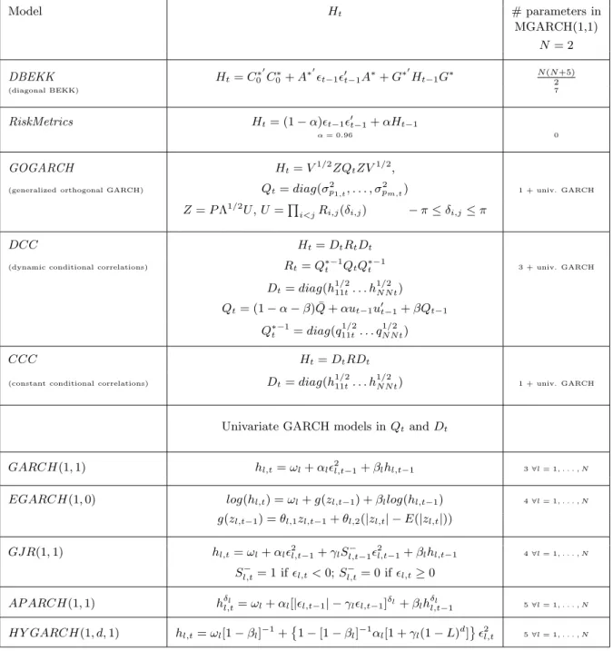
prac-tice. For the simulation study, we take a slightly different forecasting models set made up of 10 models, details are in Section 5, in order to control for the degree of similarity between models. The specifications considered in this paper are: the diagonal BEKK of Engle and Kroner (1995) and the multivariate RiskMetrics procedure, J.P.Morgan (1996), developed by J.P. Morgan. The set also includes four variations of the Constant Correlation (CCC) model (Bollerslev, 1990), of the Dynamic Conditional Correlation (DCC) model of Engle (2002), and of the Generalized Or-thogonal GARCH (GOGARCH) model of van der Weide (2002), with GARCH (Bollerslev, 1986), GJR (Glosten, Jagannathan, and Runkle, 1992), Exponencial GARCH (Nelson, 1991), Asymmet-ric Power ARCH (Ding, Granger, and Engle, 1993), Integrated GARCH (Engle and Bollerslev, 1986), RiskMetrics (J.P.Morgan,1996) and Hyperbolic GARCH (Davidson, 2004) specifications for the conditional variance equations. In the GJR model, the impact of squared innovations on the conditional variance is different when the innovation is positive or negative. The asymmet-ric power ARCH model (APARCH) is a general specification which includes seven other ARCH extensions as special cases. The Exponential GARCH model (EGARCH) accomodates the asym-metric relation between shocks and volatility by expressing the latter as a function of both the

magnitude and the sign of the shock. The Integrated GARCH (IGARCH) model is a variation of the GARCH model in which the sum of the variance parameters are constrained to be equal to one, while the RiskMetrics model (RM) is basically an IGARCH model where the constant is set to zero and the ARCH and GARCH coefficients are fixed ex ante. Finally, the Hyperbolic GARCH model (HYGARCH) allows to account for long run dependence in the volatility. The

functional forms for H_t are briefly defined in Table 1. See Bauwens, Laurent, and Rombouts

(2006) for further details. All the specifications are characterized by a constant conditional mean and the models are estimated by quasi maximum likelihood using G@RCH 5.0 (Laurent, 2007). The sample log-likelihood is given by (up to a constant)

−1 2 T t=1 log|Hit| − 1 2 T t=1 (rt−μ) H_it−1(rt−μ), (23)

and we maximize numerically forμand the parameters inH_t.

4

A proxy for the conditional variance matrix

An interesting aspect of volatility is that it becomes observable ex-post. Recent literature has focused on defining a theoretical framework for the estimation of the conditional variance of financial assets returns, which is essentially based on the analysis of high frequency data. McAller and Medeiros (2008) provide a survey on this subject. Following Andersen, Bollerslev, Diebold,

and Labys (2003), we rely on the realized covariance (RCov) to proxy the ex post variance. In

the ideal case of no microstructure noise, this measure, being based on intraday observations, is characterized by a degree of accuracy that decreases as sampling frequency lowers.

Let us assume the observed return vector to be generated by a conditionally normal

N-dimensional log-price diffusiondy(u) and a (N(N+ 1)/2)-dimensional covariance diffusiondσ(u),

with σ(u) = vech(Σ(u)) = [σij(u)] fori, j = 1, ..., N, i≥j and u∈[t, t+ 1], with mean vector

process b(u)du and covariance matrix a(u) =s(u)s(u), driven by a N(N + 3)/2 vector of

inde-pendent standard Brownian motionsW(u). Hence the diffusion process of the system admits the

following representation ⎡ ⎣ dy(u) dσ(u) ⎤ ⎦=b(u)du+s(u)dW(u), (24)

withb(u) ands(u) locally bounded and measurable. Consider now the following partition for the

covariance matrix of the system in (24) as

a(u) =s(u)s(u) = ⎡ ⎣ Σ(u) Cov(dyu, dσu) Cov(dyu, dσu) V ar(dσu) ⎤ ⎦. (25)

Table 1: Summary of the forecasting models set Model Ht # parameters in MGARCH(1,1) N = 2 DBEKK Ht=C∗ 0 C0∗+A∗t−1t−1A∗+G∗ Ht−1G∗ N(N₂+5) (diagonal BEKK) 7 RiskMetrics Ht= (1−α)t−1t−1+αHt−1 α= 0.96 0 GOGARCH Ht=V1/2ZQtZV1/2,

(generalized orthogonal GARCH) Qt=diag(σ2p1,t, . . . , σ2pm,t) 1 + univ. GARCH

Z=PΛ1/2_{U,U =}

i<jRi,j(δi,j) −π≤δi,j≤π

DCC Ht=DtRtDt

(dynamic conditional correlations) Rt=Q∗−1t QtQ∗−1t 3 + univ. GARCH

Dt=diag(h111/2t. . . h 1/2 NNt) Qt= (1−α−β) ¯Q+αut−1ut−1+βQt−1 Q_t∗−1=diag(q₁₁1/_t2. . . q1_NNt/2 ) CCC Ht=DtRDt

(constant conditional correlations) Dt=diag(h1₁₁/2t. . . h1 /2

NNt) 1 + univ. GARCH

Univariate GARCH models inQtandDt

GARCH(1,1) hl,t=ωl+αl2l,t−1+βlhl,t−1 3∀l= 1, . . . , N

EGARCH(1,0) log(hl,t) =ωl+g(zl,t−1) +βllog(hl,t−1) 4∀l= 1, . . . , N

g(zl,t−1) =θl,1zl,t−1+θl,2(|zl,t| −E(|zl,t|)) GJR(1,1) hl,t=ωl+αl2l,t−1+γlS−l,t−12l,t−1+βlhl,t−1 4∀l= 1, . . . , N S_l,t− = 1 ifl,t<0;Sl,t− = 0 ifl,t≥0 AP ARCH(1,1) hδ_l,tl =ωl+αl[|l,t−1| −γll,t−1]δl_+βlhδl l,t−1 5∀l= 1, . . . , N HY GARCH(1, d,1) hl,t=ωl[1−βl]−1+ 1−[1−βl]−1αl[1 +γl(1−L)d] 2_l,t 5∀l= 1, . . . , N

Since Σu identifies the continuous time process for the covariance matrix of the returns, we can define the Integrated Covariance (ICov) as (see Barndorff-Nielsen and Shephard, 2004)

ICov_t+1=

_t+1 t

Σ(u)du. (26)

Let us now define the intraday returns asrt+Δ=yt+Δ−ytfort= Δ,2Δ, ..., T and Δ = 1/m,

where mis the number of intervals per day. In this setting ICovt can be consistently estimated

by the Realized Covariance (RCov) (Andersen, Bollerslev, Diebold, and Labys, 2003) which is

defined as

RCovt+1,Δ=

1/Δ

i=1

rt+iΔrt+iΔ. (27)

In fact, since the process defined by (24) does not allow for jumps in the returns, it holds that plim

Δ→0RCovt+1,Δ=ICovt+1. (28)

In this paper, theRCovserves as a proxy for the true conditional variance matrix when evaluating

the forecasting performance of the different MGARCH models. The result (28) suggests that the

higher is the intraday frequency used to compute RCov, and hence the amount of information

available, the higher the accuracy of the proxy.

However, as noted by Andersen, Bollerslev, Diebold, and Labys (2003), positive definiteness

of the covariance matrix is ensured only if the number of assets is larger thenm(wherem is the

number of intervals per day). When this condition is violated then the realized covariance matrix

fails to be of full rank (i.e. rank(Rcov) =m < dim(RCov)) andRCovwill meet only the weaker

requirement to be semi-positive definite.

5

Simulation study

We investigate the ranking of the MGARCH models with respect to two main dimensions: the quality of the volatility proxy and the choice of the loss function. As expected, we find that if the quality of the proxy is good, both consistent and inconsistent loss functions rank properly. However, when the quality of the proxy is poor, only the consistent loss functions rank properly. Our findings also hold when the sample size in the estimation period increases.

5.1

Setup

Varying the quality of the proxy requires the simulation of a multivariate diffusion process. For our simulation, we select the bivariate CCC-EGARCH(1,0) model (see Table 1) which admits a diffusion limit of the type introduced by (24), defined by the continuous time vector stochastic

process [y₁t, y2t, log(σ12t), log(σ22t)], with drift and scale given respectively by b(y,Σ) = ⎡ ⎢ ⎢ ⎢ ⎢ ⎢ ⎢ ⎣ 0 0 ω1−θ1log(σ₁2_t) ω2−θ2log(σ₂2_t) ⎤ ⎥ ⎥ ⎥ ⎥ ⎥ ⎥ ⎦ (29) and a(y,Σ) = s(y,Σ)s(y,Σ) = ⎡ ⎢ ⎢ ⎢ ⎢ ⎢ ⎢ ⎣ σ₁2_t ρσ₁tσ2t α1σ1t ρα2σ1t ρσ₁tσ2t σ22t ρα1σ2t α2σ2t α1σ1t ρα1σ2t α21+γ12(1−2/π) ρα1α2+γ1γ2C ρα₂σ_1t α₂σ_2t ρα₁α₂+γ₁γ₂C α2₂+γ₂2(1−2/π) ⎤ ⎥ ⎥ ⎥ ⎥ ⎥ ⎥ ⎦ , (30)

whereC= 2_π1−ρ2+ρarcsin(ρ)−1 . The conditional covariance is computed, at each point

in time asσ_(1,2),t=ρ

σ2_1,tσ₂2_,t. The matrixs(y,Σ) is computed froma(y,Σ) by spectral

decom-position.

The CCCEGARCH specification has been preferred to alternative MGARCH specifications -e.g. the DCC model - because it is sufficient to ensure a certain degree of dissimilarity between the true DGP and the set of models while keeping the limiting diffusion fairly tractable.

For the simulation study we use the following parameter values: ωi=−0.02,θi= 1−βi= 0.03,

αi =−0.09,γi = 0.4 and ρ= 0.9. Our results are based on 500 replications with an estimation

sample of 2000 observations and a forecasting sample of T=500 observations. The continuous time process of (24) is approximated by generating 7200 observations per day - i.e. 5 observations per minute. The set of MGARCH models is estimated on daily returns and recursive 1-step ahead forecasts are computed.

The true conditional covariance matrix is measured by the integrated covariance (ICov) defined

in (26). To proxy the daily covariance matrix, we use the realized covariance (RCovt,Δ), as defined

in (27), based on intraday returns sampled at 14 different frequencies, ranging from 1 minute (most accurate) to 24 hour (least accurate), over the forecasting horizon. It is important to stress that given the bivariate DGP we should in principle stop at the 12 hour frequency to ensure a positive

definite realized variance matrix at timet. Though, when reporting our simulation results next,

we also include the 24 hour frequency to investigate what happens when a realized variance matrix which is not positive definite enters the loss functions.

As underlined by Hafner (2007) it is difficult to derive temporal aggregation results for the

process generated by (24) and (29)-(30) due to the non-linearity of the variance matrix Σt. The

to generate continuous time paths such that the resulting RCov estimators, at different time

sampling frequencies, are consistent for ICov. Contrary to the previous literature, the diffusion

approximation we introduce here allows to control better for the nature and the size of the leverage

effect and to preserve the correlation structure of the vector stochastic process [y1t, ..., σ21t, ...]

ensuring internal consistency of the model.

Note that since we are comparing estimated models, the underlying order, other than for the best model, is unknown. The initial set of models is defined such that all models are expected to be inferior. Apart from the CCC-EGARCH(1,0), the set of models includes the diagonal BEKK, Risk-Metrics, CCC-GARCH(1,1), CCC-IGARCH(1,1), CCC-RiskRisk-Metrics, GOGARCH-GARCH(1,1), GOGARCH-EGARCH(1,0), GOGARCH-IGARCH(1,1) and GOGARCH-HYGARCH(1,1).

The considered loss functions and their classification are summarized in Table 2. Table 2: Classification of the loss functions

Matrix Norms (MN) Type Transform. of MN Type

p-norm (p=1) inconsistent p-norm (p=1) squared consistent

Frobenius norm inconsistent Frobenius norm squared consistent

Eigenvalue norm inconsistent Eigenvalue norm squared consistent

5.2

Sample performance ranking and objective bias

We focus first on the ability of the loss function to detect the true model as the best. We compute the frequencies at which each model shows the smallest sample performance where the latter is

defined as the mean value of the loss functionT−1 _TL(Σt, Hit).

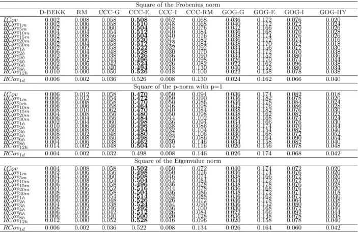
Table 3 reports these frequencies for the consistent loss functions: the squares of the Frobenius

norm, the p-norm with p = 1 and of the eigenvalue norm. Unsurprisingly, we find the

CCC-EGARCH model ranking first most often for all consistent loss functions at all frequencies for

RCov. WhenICovis used, this frequency is about 51%. The remaining 49% is distributed among

the other models (from 0% to 7%) in such a way that no model dominates. One exception is the GOGARCH-EGARCH (17%) which is not surprising since this model is the only one in the set that allows for a leverage effect. Note that the frequency associated to the GOGARCH-EGARCH is

stable acrossRCovfrequencies, that is, it only represents the ability of the GOGARCH-EGARCH

to mimic the dynamics in the covariance structure generated by the true DGP.

The fact that frequencies associated to the true model seem low when the loss is computed with respect to the true covariance is explained by the fact that we allow for a fairly high degree of similarity between models. The true CCC-EGARCH model with a moderate leverage effect can also be accounted for by other models in the set. However, the presence of the leverage effect in the DGP should imply that all symmetric models are detected as inferior. From Table 3 we also learn

that when the quality of the proxy deteriorates (the sampling frequency decreases), the sample

performance is invariant, showing the consistency of the ranking of the loss functions acrossRCov

frequencies. The informative content of the loss function is therefore independent from the proxy quality allowing to correctly order the models only on the basis of their forecasting ability.

An interesting case is the CCC-RM. The frequencies associated to the CCC-RM increase

progressively from about 8% atICovto about 10% at RCov_12h revealing a behavior that, as we

will see in the following, is typically due to the presence of the objective bias. However, the set of models includes also the CCC-IGARCH, a model which shares most of the characteristics of the CCC-RM. The frequencies of the CCC-IGARCH decrease from 5% to 1.5% in such a way to

compensate, at eachRCov frequency, the increase in the frequency associated to the CCC-RM.

The joint probability of CCC-IGARCH and CCC-RM to rank first is indeed about 13% and is

constant acrossRCov.

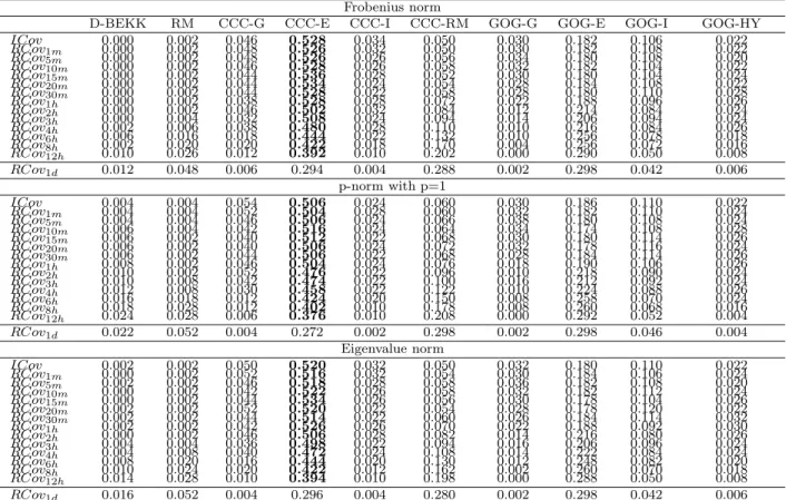
Table 4 reports the same frequencies but for the inconsistent loss functions, i.e. the Frobenius

norm, the p-norm withp= 1 and the eigenvalue norm. Recall that, when using the true volatility

(ICov), these loss functions deliver the true ranking. Indeed, the CCC-EGARCH is correctly

detected as the best model in 53% of the cases. When relying on RCov_1m to RCov_1h, the

frequencies associated to each model remain stable and there is no dominant model other than CCC-EGARCH. Hence, there is no evidence of the presence of objective bias. Starting from

RCov₂h, the frequency at which the CCC-EGARCH model ranks first starts declining while the

performance of potentially inferior models increases rapidly as the quality of the proxy lowers. The CCC-EGARCH frequency drops from about 52% to about 38% and 28% at the 12h and daily frequency respectively. Interestingly, for lower levels of proxy quality other inferior models seem to emerge, namely the GOGARCH-EGARCH and the CCC-RM. These models rank first in 18% and

about 5% of the cases respectively when using RCov computed from very high frequency data.

When using 12h returns to proxy the unobservable covariance (i.e. RCov12h) these frequencies

increase to about 29% and 20% respectively, meaning that these models rank first quite often.

This improvement in the sample performance of these models, as the frequency of RCovlowers,

signals the presence of objective bias.

In the first part of the analysis we focused on the detection of the best model in terms of sample performance. However, the analysis carried out so far, offers only a partial insight on the role of the objective bias. Indeed, in presence of a high degree of dissimilarity between the true and the competing models, the detection of the best model may not be affected by the presence of the objective bias. However, the objective bias may still be relevant for what concerns the other positions in the ranking. We now investigate whether the whole ordering is preserved despite the deterioration of the quality of the proxy. Since we are ranking over a set of estimated volatility models, the true ranking, except for the best model, is not known ex ante. However the underlying

Table 3: Frequencies at which each model shows the smallest sample loss: consistent loss functions

Square of the Frobenius norm

D-BEKK RM CCC-G CCC-E CCC-I CCC-RM GOG-G GOG-E GOG-I GOG-HY

ICov 0.002 0.008 0.058 0.508 0.052 0.068 0.036 0.172 0.076 0.020 RCov1m 0.002 0.006 0.058 0.510 0.048 0.068 0.040 0.172 0.072 0.024 RCov₅m 0.002 0.006 0.060 0.504 0.048 0.076 0.042 0.166 0.070 0.026 RCov₁₀m 0.004 0.004 0.054 0.512 0.040 0.084 0.036 0.168 0.070 0.028 RCov15m 0.002 0.008 0.056 0.504 0.040 0.076 0.038 0.174 0.076 0.026 RCov20m 0.002 0.006 0.048 0.520 0.044 0.082 0.036 0.172 0.074 0.016 RCov30m 0.002 0.004 0.058 0.512 0.042 0.084 0.038 0.170 0.072 0.018 RCov_1h 0.002 0.002 0.058 0.522 0.032 0.092 0.034 0.156 0.072 0.030 RCov_2h 0.006 0.004 0.048 0.528 0.030 0.070 0.034 0.172 0.070 0.038 RCov₃h 0.002 0.006 0.038 0.526 0.036 0.090 0.034 0.152 0.080 0.036 RCov₄h 0.006 0.002 0.044 0.496 0.040 0.098 0.026 0.170 0.074 0.044 RCov₆h 0.002 0.006 0.042 0.524 0.026 0.082 0.022 0.162 0.096 0.038 RCov₈h 0.006 0.006 0.040 0.494 0.018 0.130 0.040 0.152 0.080 0.034 RCov_12h 0.010 0.000 0.050 0.526 0.018 0.100 0.022 0.158 0.078 0.038 RCov₁d 0.006 0.002 0.036 0.526 0.008 0.130 0.024 0.162 0.066 0.040 Square of the p-norm with p=1

ICov 0.006 0.012 0.058 0.470 0.050 0.094 0.036 0.174 0.082 0.018 RCov1m 0.006 0.012 0.054 0.472 0.050 0.090 0.036 0.182 0.078 0.020 RCov5m 0.006 0.008 0.058 0.470 0.050 0.086 0.036 0.178 0.084 0.024 RCov₁₀m 0.006 0.006 0.058 0.464 0.046 0.098 0.032 0.176 0.086 0.028 RCov15m 0.008 0.010 0.062 0.470 0.040 0.084 0.038 0.182 0.076 0.030 RCov20m 0.004 0.008 0.056 0.480 0.050 0.098 0.038 0.162 0.082 0.022 RCov30m 0.006 0.004 0.056 0.484 0.044 0.102 0.038 0.168 0.074 0.024 RCov₁h 0.002 0.004 0.060 0.498 0.036 0.094 0.034 0.166 0.076 0.030 RCov_2h 0.010 0.006 0.046 0.496 0.038 0.086 0.030 0.174 0.070 0.044 RCov_3h 0.006 0.008 0.050 0.494 0.032 0.104 0.030 0.154 0.082 0.040 RCov₄h 0.008 0.002 0.048 0.480 0.034 0.106 0.030 0.168 0.072 0.052 RCov₆h 0.008 0.008 0.050 0.498 0.022 0.086 0.020 0.164 0.090 0.054 RCov₈h 0.004 0.006 0.038 0.462 0.030 0.146 0.034 0.158 0.082 0.040 RCov_12h 0.014 0.002 0.048 0.504 0.014 0.116 0.020 0.156 0.078 0.048 RCov_1d 0.004 0.002 0.032 0.498 0.008 0.146 0.026 0.174 0.068 0.042 Square of the Eigenvalue norm

ICov 0.004 0.008 0.058 0.502 0.050 0.072 0.040 0.174 0.072 0.020 RCov1m 0.002 0.006 0.056 0.498 0.050 0.076 0.036 0.174 0.076 0.026 RCov5m 0.004 0.006 0.060 0.508 0.046 0.074 0.038 0.166 0.072 0.026 RCov₁₀m 0.004 0.008 0.054 0.504 0.042 0.084 0.034 0.172 0.072 0.026 RCov₁₅m 0.006 0.006 0.058 0.496 0.036 0.078 0.038 0.178 0.076 0.028 RCov20m 0.004 0.006 0.052 0.516 0.044 0.078 0.036 0.168 0.076 0.020 RCov30m 0.008 0.006 0.058 0.504 0.036 0.086 0.038 0.172 0.074 0.018 RCov₁h 0.006 0.006 0.054 0.514 0.032 0.088 0.036 0.162 0.072 0.030 RCov_2h 0.006 0.006 0.048 0.526 0.026 0.072 0.036 0.178 0.064 0.038 RCov₃h 0.004 0.006 0.038 0.524 0.034 0.090 0.036 0.152 0.080 0.036 RCov₄h 0.008 0.002 0.046 0.492 0.036 0.100 0.030 0.168 0.072 0.046 RCov₆h 0.006 0.006 0.042 0.512 0.026 0.084 0.022 0.166 0.092 0.044 RCov₈h 0.006 0.006 0.040 0.500 0.020 0.128 0.036 0.148 0.078 0.038 RCov₁₂h 0.012 0.000 0.052 0.528 0.016 0.096 0.020 0.158 0.078 0.040 RCov_1d 0.006 0.002 0.036 0.522 0.008 0.134 0.026 0.164 0.060 0.042 Note: D-BEKK: Diagonal BEKK; RM: RiskMetrics; CCC-G,-E,-I,-RM: Constant Conditional Correlation with GARCH, EGARCH, IGARCH and Riskmetrics univariate conditional variances; GOG-G,-E,-I,-HY: Generalized Orthogonal GARCH with GARCH, EGARCH, IGARCH and HYGARCH univariate conditional variances. RCov_1dis separated by a horizontal line indicating that the realized covariance matrix is not positive definite at the daily frequency.

Table 4: Frequencies at which each model shows the smallest sample loss: inconsistent loss func-tions

Frobenius norm

D-BEKK RM CCC-G CCC-E CCC-I CCC-RM GOG-G GOG-E GOG-I GOG-HY

ICov 0.000 0.002 0.046 0.528 0.034 0.050 0.030 0.182 0.106 0.022 RCov1m 0.000 0.002 0.048 0.526 0.032 0.050 0.030 0.182 0.108 0.022 RCov₅m 0.000 0.002 0.048 0.526 0.026 0.056 0.034 0.180 0.108 0.020 RCov₁₀m 0.000 0.002 0.046 0.528 0.026 0.058 0.032 0.182 0.104 0.022 RCov15m 0.000 0.002 0.044 0.536 0.028 0.052 0.030 0.180 0.104 0.024 RCov20m 0.000 0.002 0.044 0.534 0.024 0.054 0.028 0.184 0.108 0.022 RCov30m 0.000 0.002 0.044 0.528 0.022 0.058 0.028 0.180 0.110 0.028 RCov_1h 0.000 0.002 0.038 0.528 0.028 0.072 0.022 0.188 0.096 0.026 RCov_2h 0.000 0.002 0.046 0.502 0.032 0.084 0.012 0.214 0.084 0.024 RCov₃h 0.000 0.004 0.032 0.508 0.024 0.094 0.014 0.206 0.094 0.024 RCov₄h 0.002 0.006 0.038 0.480 0.028 0.110 0.010 0.216 0.084 0.026 RCov₆h 0.006 0.016 0.018 0.444 0.022 0.132 0.010 0.256 0.078 0.018 RCov_8h 0.002 0.020 0.020 0.422 0.018 0.170 0.004 0.256 0.072 0.016 RCov_12h 0.010 0.026 0.012 0.392 0.010 0.202 0.000 0.290 0.050 0.008 RCov₁d 0.012 0.048 0.006 0.294 0.004 0.288 0.002 0.298 0.042 0.006 p-norm with p=1 ICov 0.004 0.004 0.054 0.506 0.024 0.060 0.030 0.186 0.110 0.022 RCov1m 0.004 0.004 0.052 0.504 0.028 0.060 0.032 0.182 0.110 0.024 RCov₅m 0.004 0.004 0.046 0.506 0.024 0.066 0.038 0.180 0.108 0.024 RCov₁₀m 0.006 0.004 0.042 0.516 0.024 0.064 0.034 0.174 0.108 0.028 RCov15m 0.006 0.002 0.040 0.512 0.022 0.068 0.030 0.180 0.114 0.026 RCov20m 0.006 0.002 0.040 0.506 0.024 0.072 0.032 0.178 0.116 0.024 RCov30m 0.006 0.002 0.044 0.506 0.022 0.068 0.028 0.184 0.114 0.026 RCov₁h 0.008 0.002 0.046 0.504 0.024 0.076 0.018 0.190 0.106 0.026 RCov_2h 0.010 0.002 0.052 0.476 0.022 0.096 0.010 0.218 0.090 0.024 RCov₃h 0.010 0.008 0.042 0.474 0.022 0.100 0.016 0.212 0.092 0.024 RCov₄h 0.012 0.008 0.030 0.458 0.022 0.122 0.010 0.224 0.088 0.026 RCov₆h 0.016 0.018 0.012 0.424 0.020 0.150 0.008 0.258 0.070 0.024 RCov₈h 0.018 0.028 0.012 0.402 0.010 0.178 0.008 0.260 0.068 0.016 RCov_12h 0.024 0.028 0.006 0.376 0.010 0.208 0.000 0.292 0.052 0.004 RCov₁d 0.022 0.052 0.004 0.272 0.002 0.298 0.002 0.298 0.046 0.004 Eigenvalue norm ICov 0.002 0.002 0.050 0.520 0.032 0.050 0.032 0.180 0.110 0.022 RCov1m 0.000 0.002 0.052 0.516 0.032 0.054 0.030 0.184 0.106 0.024 RCov5m 0.002 0.002 0.046 0.518 0.028 0.058 0.036 0.182 0.108 0.020 RCov₁₀m 0.000 0.002 0.042 0.522 0.026 0.058 0.032 0.182 0.112 0.024 RCov15m 0.000 0.002 0.044 0.534 0.026 0.056 0.030 0.178 0.104 0.026 RCov20m 0.002 0.002 0.052 0.520 0.022 0.054 0.028 0.178 0.120 0.022 RCov30m 0.002 0.002 0.044 0.514 0.022 0.060 0.026 0.184 0.114 0.032 RCov₁h 0.002 0.002 0.042 0.526 0.026 0.070 0.022 0.188 0.092 0.030 RCov_2h 0.000 0.002 0.046 0.506 0.028 0.082 0.014 0.216 0.080 0.026 RCov₃h 0.004 0.004 0.036 0.498 0.022 0.094 0.016 0.206 0.096 0.024 RCov₄h 0.004 0.008 0.040 0.472 0.024 0.108 0.014 0.222 0.084 0.024 RCov₆h 0.008 0.020 0.016 0.444 0.020 0.130 0.012 0.248 0.082 0.020 RCov₈h 0.010 0.024 0.020 0.422 0.012 0.162 0.002 0.260 0.070 0.018 RCov_12h 0.014 0.028 0.010 0.394 0.010 0.198 0.000 0.288 0.050 0.008 RCov_1d 0.016 0.052 0.004 0.296 0.004 0.280 0.002 0.298 0.042 0.006 Note: D-BEKK: Diagonal BEKK; RM: RiskMetrics; CCC-G,-E,-I,-RM: Constant Conditional Correlation with GARCH, EGARCH, IGARCH and Riskmetrics univariate conditional variances; GOG-G,-E,-I,-HY: Generalized Orthogonal GARCH with GARCH, EGARCH, IGARCH and HYGARCH univariate conditional variances. RCov_1dis separated by a horizontal line indicating that the realized covariance matrix is not positive definite at the daily frequency.

ordering implied by a given loss function, can be identified by ranking the models with respect to

the true covarianceICov.

A general result appears from Tables 3 and 4. Unsurprisingly, the frequencies reported are homogeneous between loss functions within each group. This is a direct result of the equivalences stated in (5) and (20), for the consistent, (11) and (21) for the inconsistent loss functions. Hence, without loss of generality, we consider next only one consistent (Frobenius norm squared) and one inconsistent (Frobenius norm) loss function. Figure 1(a) shows the ranking based on the average performance (over the 500 replications) implied by the consistent loss function for various levels

of proxy quality. This ranking is fairly stable acrossRCovfrequencies meaning that the squared

Frobenius norm is able to consistently order models even when the quality of the proxy deteriorates. Shifts in position affect only the middle of the classification and can be justified by the extremely

close average sample performances between the models, with differences atRCov1d smaller than

10−2 (Figure 1(b)). Figures 1(b) and 1(c) provide some insights to disentangle the role of the

accuracy of the covariance proxy. Figure 1(c) reports models average performances normalized to the average performance of the CCC-EGARCH model. The converging pattern towards the

true model, together with constant deviations between models across RCov frequencies (Figure

1(b)) suggests that the loss of accuracy only translates into a increase in the level of the average sample performances for all models. Constant discrepancies between models imply that not only the ordering but also the degree of similarity, and therefore the relationships between models, are preserved across frequencies. However, the increase in the variability of the proxy induces an increase in the variability of the loss function which, in empirical applications, may result in the impossibility to effectively discriminate between models.

A different picture emerges when considering the inconsistent loss function (Figure 2(a)). In this case, the ranking is preserved up to one hour sampling frequency. Due to the appearance of the objective bias, we observe major shifts at lower frequencies at most levels of the classification. The impact of the objective bias is amplified by the fact that except for the first two positions, i.e. CCC-EGARCH and GOGARCH-EGARCH, all the other models exhibit very close average

sample performances (Figure 2(b)), with differences smaller than 10−2atRCov₁d. Inferior models

like RiskMetrics and CCC-RM, 10th and 9th respectively according toICov, improve up to the

3rd and 2nd positions respectively. The CCC-EGARCH is classified as the best forecasting model at all frequencies, followed by the GOGARCH-EGARCH. This result is due to the fact that these two models are sufficiently different from the others (they are the only models in the set to allow for leverage effect of the same type as implied by the true model), with the CCC-EGARCH clearly dominating the GOGARCH-EGARCH (Figure 2(b)). Although the objective bias does not become an issue when ordering between these two models, Figure 2(b) shows that, as the frequency

performance. Since, as underlined above, the variability of the loss function increases along with the variability of the proxy, the probability to rank the GOGARCH-EGARCH first increases at low frequences. This conclusion is consistent with the results reported in Table 4.

Besides varying the proxy quality and studying several loss functions we also investigate the impact of the estimation sample size on the rankings. We increase the sample size by 50% to 3000 observations and we find qualitatively identical results (results available on request).

6

Empirical application

6.1

Data description and estimation results

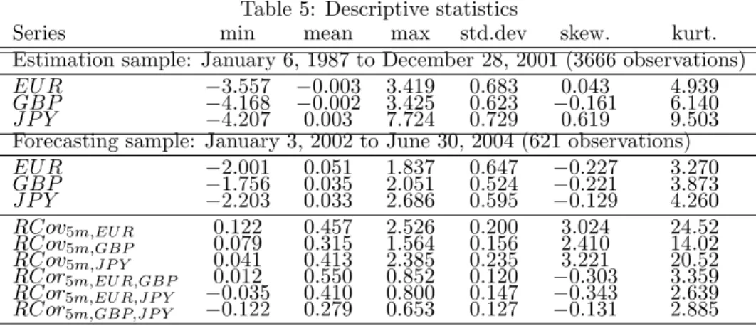
The empirical application is based on the Euro, British Pound and the Japanese Yen exchange rates expressed in US dollars (EUR, GBP and JPY). The sample period is January 6, 1987 through June 30, 2004 totaling 4287 trading days. Intraday returns and realized covariances are computed from five-minutes intervals last mid-quotes, implying 288 intraday observations. The data have been provided by Olsen & Associates. Missing values are replaced by linearly interpolating the closest previous and the first following 5-minute price. The dataset has been cleaned from weekends, holidays and early closing days. Days with too many missing values and/or constant prices are also removed. Five-minute returns are computed as the first difference of the logarithmic prices. The estimation sample ranges from January 6, 1987 to December 28, 2001 (3666 trading days), while the remaining observations (621 trading days) are used for the out-of-sample forecasts evaluation. Table 5 reports descriptive statistics for the estimation sample and the forecasting sample. With respect to the daily frequency, the EUR and GBP exchange rates share similar data characteristics and are relatively highly correlated. JPY has quite a higher kurtosis and a more pronounced skewness. The 5-minute realized variances and correlations are quite dispersed. For example the correlations vary between -0.12 and 0.85. We also remark that the variances are positively skewed and the correlations negatively skewed.

The proxy for the conditional covariance is realized covariance (RCov) as defined in (27)

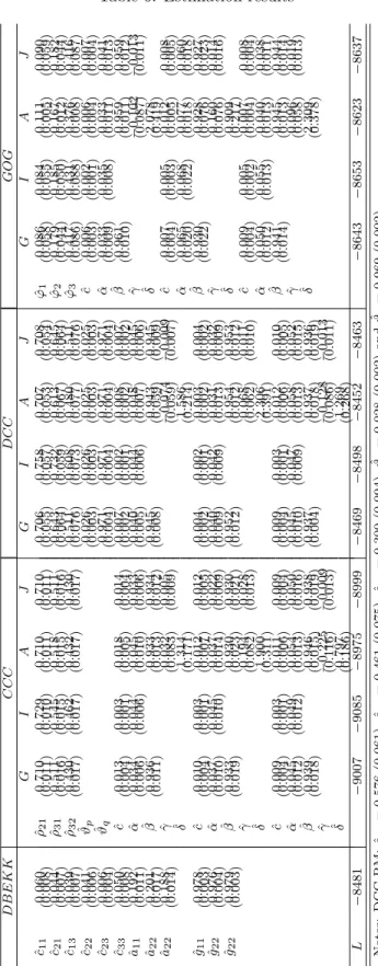
computed at 14 different frequencies ranging from 5 min. to 24 h. We stress again, like in the simulation study, that we should stop at the 8h frequency if we want to have a positive definite realized variance matrix at each point in time. We include the results until the 24h frequency to illustrate what happens when the realized variance matrix is not positive definite. One-step-ahead forecasts are computed from 4:05 pm to 4:00 pm ET and are contrasted to the realized measure of volatility using one consistent (Frobenius norm squared) and one inconsistent (Frobenius norm) loss function. Estimation results for the 16 MGARCH models are reported in Table 6. Note that there is no Riskmetrics and CCC-RM procedures reported in Table 6 since they do not require parameter estimation (the sample correlation is used for the CCC-RM). Generally speaking, we

Figure 1: Consistency of the ranking based on average performance - Frobenius norm squared 1 2 3 4 5 6 7 8 9 10 ∞ 1m 5m 10m 15m 20m 30m 1h 2h 3h 4h 6h 8h 12h 1d CCC−EGARCH GOG−EGARCH CCC−GARCH CCC−IGARCH GOG−IGARCH CCC−RM RiskMetrics D−BEKK GOG−GARCH GOG−HYGARCH

Ranking based on average performances

RCov (a) Ranking based on average performances

0.0 0.1 0.2 0.3 0.4 0.5 0.6 0.7 0.8 ∞ 1m 5m 10m 15m 20m 30m 1h 2h 3h 4h 6h 8h 12h 1d D−BEKK RiskMetrics CCC−GARCH CCC−EGARCH CCC−IGARCH CCC−RM GOG−GARCH GOG−EGARCH GOG−IGARCH GOG−HYGARCH

Average performances (deviations)

RCov (b) Avg. performances - Deviations from the CCC-EGARCH

1.00 1.05 1.10 1.15 1.20 1.25 1.30 1.35 ∞ 1m 5m 10m 15m 20m 30m 1h 2h 3h 4h 6h 8h 12h 1d D−BEKK RiskMetrics CCC−GARCH CCC−EGARCH CCC−IGARCH CCC−RM GOG−GARCH GOG−EGARCH GOG−IGARCH GOG−HYGARCH

Normalized average performances

RCov (c) Normalized average performances

Figure 2: Consistency of the ranking based on average performance - Frobenius norm 1 2 3 4 5 6 7 8 9 10 ∞ 1m 5m 10m 15m 20m 30m 1h 2h 3h 4h 6h 8h 12h 1d CCC−EGARCH GOG−EGARCH CCC−GARCH GOG−IGARCH CCC−IGARCH GOG−GARCH GOG−HYGARCH D−BEKK CCC−RM RiskMetrics

Ranking based on average performance

RCov (a) Ranking based on average performances

0.00 0.02 0.04 0.06 0.08 0.10 0.12 ∞ 1m 5m 10m 15m 20m 30m 1h 2h 3h 4h 6h 8h 12h 1d D−BEKK RiskMetrics CCC−GARCH CCC−EGARCH CCC−IGARCH CCC−RM GOG−GARCH GOG−EGARCH GOG−IGARCH GOG−HYGARCH

Average performances (deviations)

RCov (b) Avg. performances - Deviations from the CCC-EGARCH

1.000 1.025 1.050 1.075 1.100 1.125 1.150 1.175 ∞ 1m 5m 10m 15m 20m 30m 1h 2h 3h 4h 6h 8h 12h 1d D−BEKK RiskMetrics CCC−GARCH CCC−EGARCH CCC−IGARCH CCC−RM GOG−GARCH GOG−EGARCH GOG−IGARCH GOG−HYGARCH

Normalized average performances

RCov (c) Normalized average performances

Table 5: Descriptive statistics

Series min mean max std.dev skew. kurt.

Estimation sample: January 6, 1987 to December 28, 2001 (3666 observations)

EU R −3.557 −0.003 3.419 0.683 0.043 4.939

GBP −4.168 −0.002 3.425 0.623 −0.161 6.140

J P Y −4.207 0.003 7.724 0.729 0.619 9.503

Forecasting sample: January 3, 2002 to June 30, 2004 (621 observations)

EU R −2.001 0.051 1.837 0.647 −0.227 3.270 GBP −1.756 0.035 2.051 0.524 −0.221 3.873 J P Y −2.203 0.033 2.686 0.595 −0.129 4.260 RCov₅m,EUR 0.122 0.457 2.526 0.200 3.024 24.52 RCov5m,GBP 0.079 0.315 1.564 0.156 2.410 14.02 RCov₅m,JP Y 0.041 0.413 2.385 0.235 3.221 20.52 RCor5m,EUR,GBP 0.012 0.550 0.852 0.120 −0.303 3.359 RCor₅m,EUR,JP Y −0.035 0.410 0.800 0.147 −0.343 2.639 RCor5m,GBP,JP Y −0.122 0.279 0.653 0.127 −0.131 2.885

The estimated correlations for the estimation sample areρEU R,GBP = 0.720,ρEU R,JP Y = 0.493 andρGBP,JP Y = 0.415. The estimated correlations for the forecasting sample are

ρEU R,GBP = 0.721,ρEU R,JP Y = 0.490 andρGBP,JP Y = 0.416.

observe that the parameters estimates for the conditional variance, covariance and correlations imply highly persistent processes. Furthermore, in almost all cases, the null of no leverage effect cannot be rejected at standard significance levels.

6.2

Model comparison

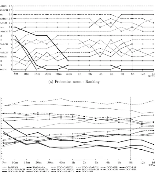
The empirical ranking of the 16 MGARCH models, as a function of the level of aggregation of

the data used to computeRCov, is reported in Figures 3 and 4. The consistent loss function in

Figure 3(a) points to the CCC-GARCH as the best forecasting model at almost all frequencies. More generally we can conclude that the subset given by both the CCC and the DCC both with GARCH and GJR outperforms all the other models. This model is followed by the CCC-GJR, with differences between the two rather negligible (Figure 3(b)). The overall ranking is well preserved across all frequencies.

The GOGARCH model is always largely dominated by all other models regardless the condi-tional variance specification. There is no clear dominance between the CCC and the DCC models and their ranking position depends on the model chosen for the conditional variance. Here the GARCH/GJR represents the best combination, followed in the order by the APARCH, the RM and finally the IGARCH. Interestingly, the three models which are based on the RiskMetrics approach, which assumes dynamics for the variance process independent of the data by fixing a smoothing parameter ex ante (RiskMetrics, CCC-RM and DCC-RM) are positioned in the middle of the classification. Figure 3(a) shows that between 10 min. and 1 h., the ranking is particularly stable but rather volatile outside this range of frequencies. The accuracy of the volatility proxy plays an important role here. As pointed out by Hansen and Lunde (2006) we can observe discrep-ancies between the empirical and the approximated ranking in finite samples (i.e. sampling error).

Table 6: Estimation results DB E K K CCC DC C GO G GI A J GI A J GI A J ˆ c11 0 . 060 ˆ ρ21 0 . 710 0 . 729 0 . 710 0 . 710 0 . 706 0 . 758 0 . 707 0 . 708 ˆ ϕ1 0 . 086 0 . 084 0 . 111 0 . 090 (0 . 008) (0 . 011) (0 . 010) (0 . 011) (0 . 011) (0 . 055) (0 . 057) (0 . 053) (0 . 054) (0 . 058) (0 . 055) (0 . 005) (0 . 059) ˆ c21 0 . 044 ˆ ρ31 0 . 511 0 . 545 0 . 518 0 . 511 0 . 643 0 . 732 0 . 613 0 . 645 ˆ ϕ2 0 . 179 0 . 185 0 . 167 0 . 182 (0 . 007) (0 . 016) (0 . 015) (0 . 015) (0 . 016) (0 . 064) (0 . 059) (0 . 067) (0 . 064) (0 . 044) (0 . 050) (0 . 012) (0 . 044) ˆ c13 0 . 039 ˆ ρ32 0 . 430 0 . 462 0 . 432 0 . 430 0 . 511 0 . 608 0 . 480 0 . 511 ˆ ϕ3 0 . 417 0 . 431 0 . 376 0 . 416 (0 . 007) (0 . 017) (0 . 017) (0 . 017) (0 . 017) (0 . 076) (0 . 073) (0 . 077) (0 . 076) (0 . 086) (0 . 088) (0 . 008) (0 . 087) ˆ c22 0 . 041 ˆϑp 0 . 026 0 . 026 0 . 025 0 . 025 ˆ c 0 . 006 0 . 002 0 . 006 0 . 007 (0 . 006) (0 . 003) (0 . 003) (0 . 003) (0 . 003) (0 . 003) (0 . 001) (0 . 004) (0 . 004) ˆ c23 0 . 006 ˆϑq 0 . 971 0 . 971 0 . 971 0 . 971 ˆ α