SHAPE REGISTRATION USING OPTIMIZATION FOR MOBILE ROBOT NAVIGATION. Feng Lu

(1)

SHAPE REGISTRATION USING OPTIMIZATION

FOR MOBILE ROBOT NAVIGATION

by

Feng Lu

A

A thesis submitted in conformity with the requirements

for the degree of Doctor of Philosophy

Graduate Department of Computer Science

University of Toronto

c

(2)

i

Shape Registration Using Optimization

For Mobile Robot Navigation

Doctor of Philosophy, 1995 Feng Lu

Department of Computer Science Univeristy of Toronto

Abstract

The theme of this thesis is shape registration (also called shape matching or shape alignment) using optimization-based algorithms. We primarily address this problem in the context of solving the mobile robot self-localization problem in unknown environments. Here the task is matching 2D laser range scans of the environment to derive the relative position and heading of the robot. The diculties in this problem are that the scans are noisy, discontinuous, not necessarily linear, and two scans taken at dierent positions may not completely overlap because of occlusion. We propose two iterative scan matching algorithms which do not require feature extraction or segmentation. Experiments demonstrate that the algorithms are eective in solving the scan matching problem.

Based on the result of aligning pairwise scans, we then study the optimal registration and inte-gration of multiple range scans for mapping an unknown environment. Here the issue of maintaining consistency in the integrated model is specically raised. We address this issue by maintaining in-dividual local frames of data and a network of uncertain spatial relations among data frames. We then formulate an optimal procedure to combine all available spatial relations to resolve possible map inconsistency. Two types of sensor data, odometry and range measurements, are used jointly to form uncertain spatial relations.

Besides the applications for mobile robots, we also study the shape registration problem in other domains. Particularly, we apply extensions of our methods for registration of 3D surfaces described by range images, and 2D shapes from intensity images.

(3)

ii

Acknowledgements

First of all, I would like to thank my supervisor, Evangelos Milios, for his continued inspiration, guidance, encouragement, and support throughout my studies. He has been conscientious in his attention to every aspect of my professional development. I owe him enormous thanks.

I thank the other members of my committee, Michael Jenkin, Allan Jepson, John Tsotsos, and my external examiner, Ingemar Cox, for the time and thought they have put into hearing my ideas and reading my thesis. Their constructive criticism has greatly improved the thesis.

I am grateful to Piotr Jasiobedzki for his advice and help on my research work and also for bringing me into the retinal image analysis project.

I beneted from the discussions with the fellow graduate students in the Vision/AI group and I am also grateful for their helps and friendship. In particular, I would like to thank Xuan Ju, Victor Lee, Yiming Ye, Richard Mann, Sean Culhane, Zhengyan Wang, Niels Lobo, David Wilkes, Chris Williams, and Evan Steeg.

I thank Songnian Zhou for his generous help and encouragement in my early years at the University of Toronto.

(4)

Introduction

1.1 Shape Registration

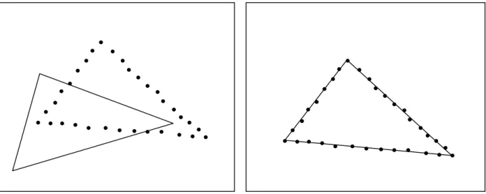
To put it simply, shape registration is to align two similar shapes, typically a data (object) shape and a model shape, by moving one around with respect to the other. We consider that two shapes are in alignment if they spatially conform with each other to achieve a minimum distance according to some distance criterion. For example, Fig. 1.1(a) shows two similar shapes misaligned with each other. A possible registration result is given in Fig. 1.1(b) where we rotated and translated one shape to make it aligned with the other shape. The type of shapes we consider here are contour curves (in 2D) and surfaces (in 3D). In this thesis, we are more concerned about the geometric alignment of shapes rather than the determination of whether the given shapes are similar, although we may obtain a measure of similarity as a by-product. Under this context, we use the terms shape registration, shape alignment, and shape matching almost interchangeably.

A typical approach to shape registration is to use distinctive features. For example, in aligning the triangles in Fig. 1.1, we may locate the corner points or the linear segments in the shapes and use them as features. By making correspondences between pairs of features on the two shapes, a registration can be determined.

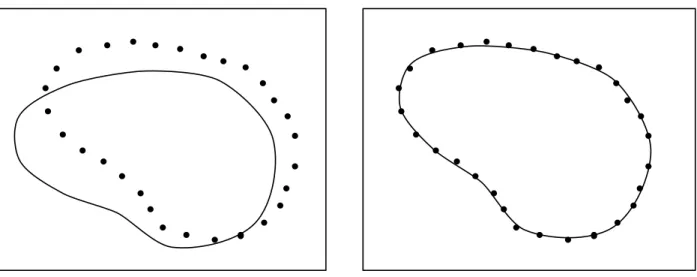
Feature-based methods may be inappropriate for matching smooth free-form shapes where it is dicult to detect distinctive features reliably. Consider the example in Fig. 1.2 and imagine how a human would align these shapes. One may draw the two shapes on separate transparencies and visually align them. After overlapping the two transparencies containing the shapes, one can try to make a series of small adjustments to the relative position and orientation to improve the alignment, and nally derive an optimal registration. This intuitive process can be achieved computationally

(10)

1.2. APPLICATIONS OF SHAPEREGISTRATION 2

a b

Figure 1.1: Shape registration. Corners or linear segments can be used as features to align these shapes.

using iterative optimization techniques. In this thesis, we will pay close attention to this type of optimization-based matching methods.

1.2 Applications of Shape Registration

Shape registration is an important problem in computer vision, especially in object recognition, motion analysis, and robot navigation.

There are many applications for shape registration. For instance, in the medical and surgical elds, various imaging sensors can provide specic information for a patient (e.g. Computed To-mography (CT), Magnetic Resonance Imaging (MRI), and 3D Ultrasound images). There is a real need to register all of these 3D images in the same reference system, and to then link these images with the operating instruments such as guiding systems or robots 76]. To achieve this goal, one possibility is to use some anatomical surfaces as references in all these images. In some cases, it becomes necessary to use a laser range nder to acquire the skin surface of a patient, and then to register this reference surface with the skin surface segmented on another imaging device.

In the industrial world, it is often required to inspect 3D parts to determine if they agree with the geometric design specications. This can be achieved by digitizing the 3D object using a high-accuracy laser range nder over a shallow depth of eld and matching the data with an

(11)

1.3. MOBILE ROBOTNAVIGATION 3

b a

Figure 1.2: The smooth free-form shapes in (a) can be registered by making a series of small adjustments to the relative position and orientation. Part (b) gives a possible registration result. ideal CAD model. Furthermore, it is also important to build integrated models from existing 3D objects. An automatic model acquisition system could signicantly improve the speed and exibility compared to conventional interactive techniques such as computer-aided geometric design (CAGD) and coordinate-measurement machines (CMM). Since a range map only samples the surface of the object which is visible from a given viewpoint, the acquisition of several range views is mandatory in order to scan the entire object. Therefore, to obtain an integrated model, it is necessary to transform and register all the partial views into a common reference frame.

1.3 Mobile Robot Navigation

The task of mobile robot navigation is to guide the vehicle through its world based on sensory information. The questions that a robot often faces are:

Where am I?

Where are other places relative to me? How do I get to other places from here?

We will address the rst question, which concerns the robot pose estimation problem, by using laser range sensing on the robot and then matching the range measurements. We will also study

(12)

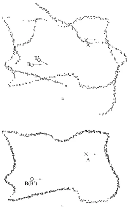
1.3. MOBILE ROBOTNAVIGATION 4 A B’ B A B(B’) a b

Figure 1.3: Example of robot pose estimation from matching range scans.

A

is a reference pose at which a reference scan (labeled as x's) is taken. The robot is now at pose

B

in reality, but thinks it is at pose

B

0 due to error. Part (a) shows that the scan at

B

(labeled with small circles) does

not align with the reference scan because of the pose error. Part (b) shows the result of aligning the two scans. The pose

B

0 is corrected to the true pose

B

at the same time.

the issue of building world models which is relevant to many aspects of navigation.

1.3.1 Robot Pose Estimation

We represent the contour of the world in a horizontal plane using a 2D curve model. Suppose that the robot is equipped with a laser range nder which rotates in the same horizontal plane and takes range measurements at many directions. If these measurements are suciently dense, the points corresponding to the intersection points of the laser beams and the world contour essentially form the same shape as the world model. Then by aligning the shape described by the data points with the model shape, we can determine the pose of the robot in the model coordinate system.

A world model may not always be available a priori to the navigation task. For example, a robot exploring an unknown environment does not have such a model to reference its position. One solution is to build a world model from previously collected sensor data and then use this model to reference the robot's new position. A simple case is to just use one previous range scan as a reference. By registering the current range scan with the reference scan, we can determine the relative pose. We will study this problem in great detail in the thesis. Here we give an example to illustrate the problem (Fig. 1.3).

(13)

1.3. MOBILE ROBOTNAVIGATION 5 robot robot d c b a

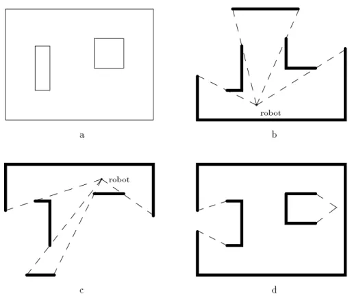
Figure 1.4: Building a world model from scans of sensor data: (a) the world being explored, (b) accumulated model so far, (c) a new scan of range data, (d) updated model.

1.3.2 Building a World Model from Sensor Data

A world model can be useful in solving problems such as path planning and robot self-localization. Acquiring a world model of an unknown environment could also be the goal of a robot's mission. A robot may build a world model by integrating successive frames of sensor data. Figure 1.4 shows an example of dynamically building a world contour map from range data.

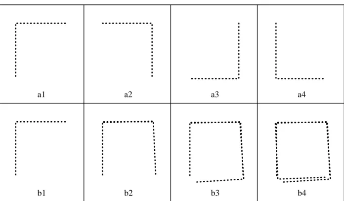
In order to integrate multiple frames of sensor data, it is essential to rst register them in a common coordinate system. A possible approach is to align each new frame of data to a previous frame or a cumulative model. But a potential problem with this approach is that the resulting model may become inconsistent as local registrations are derived independently from dierent parts of the model and there are errors in the registrations. Especially, if a long chain of registrations are compounded, there can be a signicant error in the integrated model. Figure 1.5 illustrates this problem. Although there is only a small registration error at every step of adding new data, error

(14)

1.4. THESIS OUTLINE 6

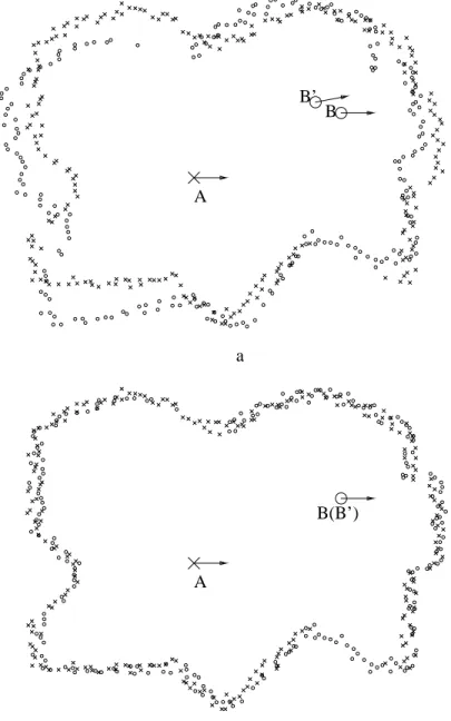
a1 a2 a3 a4

b1 b2 b3 b4

Figure 1.5: Inconsistent model due to accumulation of registration errors. (a1{a4) show local frames of sensor data from a rectangular environment. Each frame only overlaps with two adjacent frames. (b1{b4) are the cumulative models where only slight registration error is present at each step. The nal model in (b4) appears to be inconsistent in the bottom part.

accumulation leads to a signicant inconsistency in the nal model.

In this thesis, we will study the problem of integrating multiple range scans and we will specif-ically raise the issue of maintaining model consistency.

1.4 Thesis Outline

The theme of the thesis is shape registration or shape matching. We rst address this problem in the context of mobile robot applications. In particular, we propose algorithms for aligning 2D shapes of the environment which the robot observes in the form of range scans. Relative poses of the robot can be derived through the alignment of scans. Moreover, by aligning multiple scans, we can coherently integrate the range measurements for mapping the environment.

Besides the applications for robot navigation, we also study the shape registration problem in other domains. Particularly, we examine our methods as well as other techniques for registration

(15)

1.4. THESIS OUTLINE 7

of 3D surfaces described in range images and registration of 2D shapes from intensity images. Throughout the thesis, we focus on matching based on iterative optimization, as opposed to feature correspondence.

The rest of the thesis contains four parts. We give a brief outline below.

First of all, we present a literature review in Part I (Chapter 2). Areas related to our work, including robot navigation, pose estimation, robot map building, and shape registration techniques, will be surveyed. The signicance of our own work in the context of the literature will also be pointed out.

In Part II of the thesis (Chapter 3 to Chapter 5), we study the problem of robot pose estimation in unknown environments by matching range scans. We propose two iterative algorithms which can eectively align a range scan against another scan so as to derive their relative pose. Experiments using both simulated data and real data will be presented.

In Part III (Chapters 6 and 7), we study the consistent registration and integration of multi-ple range scans for mapping the environment. First, pose constraints are derived from matching pairwise scans as well as from odometry sensing, which form a network of pose relations. Then we formulate an optimal estimation procedure based on the maximum likelihood criterion to combine all the pose relations and derive the scan poses. Experiments using simulated and real data will be shown.

Part IV (Chapters 8 and 9) investigates the shape registration problem in domains other than mobile robotics, namely the registration of 3D range surfaces and 2D planar image shapes. We will examine the extensions of our algorithms (from Part II) as well as other techniques.

Finally, Chapter 10 concludes the thesis with a summary and a discussion of possible future research directions.

(16)

Review of Related Work

(17)

9 We present a literature review in the areas related to our research work. The organization of the review and its relationship with our own work are the following.

First of all, in Section 2.1, we review the topic of mobile robot navigation and particularly, robot pose estimation. This discussion gives a big picture of the area and lays a background for the thesis since our work in Part II and Part III are related to mobile robot navigation.

In Section 2.2, we specically examine existing techniques of matching sensor data for robot pose estimation. A substantial part of our own work (presented in Part II of the thesis) belongs in this area.

In Section 2.3, we discuss the types of world models used for robot pose estimation and the techniques for dynamically building models from sensor data. One issue in model building that we are particularly interested in is the global consistency in integrating sensor data. Our research work regarding this issue is presented in Part III of the thesis.

Finally, in Section 2.4, we review the general shape matching techniques in a broader domain. Shape matching is the theme throughout the thesis and it is the central issue in the problem of robot pose estimation using range data. Besides, we also study shape matching techniques for other applications such as 3D range surface registration and planar image shape registration (presented in Part IV of the thesis).

(18)

Review of Related Work

2.1 Mobile Robot Navigation

Navigation is a fundamental requirement of autonomous mobile robots. It is dened as \the sci-ence of getting ships, aircrafts, or spacecrafts from place to place esp: the method of determining position, course, and distance traveled" 91]. Navigation and position estimation has been exten-sively studied for ships, missiles, aircrafts, and spacecrafts. However, navigation for mobile robots remains a dicult problem, given the available knowledge and experience in the land, marine and aerospace communities. The reason for this is clear: it is not navigation itself that is the problem, rather it is the reliable acquisition or extraction of sensor information, and the automatic correla-tion or correspondence of these measurements with a navigacorrela-tion map that makes the autonomous navigation problem so dicult.

2.1.1 Issues in Robot Navigation

The goal of sensor-based autonomous robot navigation is to build a system which dynamically guides and controls a mobile robot from its start position to a predened end position, while avoiding known or unknown obstacles. The robot should eciently interpret data from its on-line sensors to determine its relationship to the world and the current state of the task, and then should plan and execute an appropriate course of action to accomplish the task.

Previous research in mobile robotics has typically addressed the following types of problems.

Path planning

First, path planning in a known environment is studied. The optimality criterion in this class of problems is the minimization of the cost for traversal between a start and an end position, while

(19)

avoiding obstacles 75]. A common approach is to represent the world as a graph and perform an

A

search or to apply some form of Dijkstra's algorithm to determine the shortest path. The visibility graph algorithm 81, 97] is an example in this class. Voronoi diagrams have been used to plan a path that stays away from obstacles as far as possible 21, 113]. Explicit representation of free space using overlapping cones called \freeways" is also proposed for path planning 18]. Another approach is to recursively subdivide free space into smaller cells until a collision-free path can be found through a connected set of free cells 20]. A multiresolution quadtree structure has been suggested 62] for the ecient representation of free space. The theoretical issue of path planning complexity with complete information (the \Piano Mover's Model") is studied in 104].

If environmental sensing is imperfect, uncertainty should be considered in path planning. A method using Sensory Uncertainty Field for planning a robot path that minimizes uncertainty at navigation time is proposed in 114] with preliminary results. A method which integrates dynamic path planning with self-localization and landmark extraction is discussed in 10].

Trajectory planning

Then, robot trajectory or motion planning in the presence of moving obstacles is studied. The goal is to nd an optimal robot trajectory (consisting of both a path and the motion along the path) which avoids collision with moving obstacles. Some theoretical results about the complexity of trajectory planning can be found in 100, 22]. Some heuristic approaches for planning a collision-free path in the presence of moving obstacles are presented in 46, 47, 66].

The concept of conguration space has been widely used for solving the path planning problem. Here the original problem of planning the motion of an object through a space of obstacles is transformed into an equivalent, but simpler, problem of planning the motion of a point through a space of enlarged conguration space obstacles 81, 80]. Conguration space provides an eective framework for investigating motion planning problem for robot arm manipulators 88].

Algorithmic exploration

Another type of problem is exploration of an unknown world with perfect range sensing and odometry information 87]. Here the issues are primarily the covering of the entire environment and the complexity of the algorithm as a function of the complexity of the environment (number of vertices and edges of objects). Some research work on this class of problem can be found in 97, 88, 37, 120].

(20)

Path execution and self-localization

A practical problem which has attracted much research attention is the problem of path execu-tion within a known or mostly known real environment. The focus here is typically on the sensing required to accurately execute a preplanned path, and the key problem is robot self-localization (the \where am I" problem). One primary issue in solving this problem is how to match sensed data (vision, sonar, laser, infrared etc.) against map information. A comprehensive survey of the literature in this area can be found in 30, 59]. We will discuss the robot self-localization problem in more detail in the following subsection.

Local obstacle avoidance

The issue of local obstacle avoidance arises when the world is not perfectly known. During the execution of a path, if an unexpected obstacle is encountered, the path needs to be modied or local strategies should be employed to avoid collision with the obstacle. A common approach is based on the articial potential eld 3, 67, 17, 2]. A heuristic approach for path replanning is used in 16].

Exploration with imperfect sensing

The problem of exploration of an unknown world with imperfect range sensing and odometry information is addressed 71]. The general approach is to gather sensing information and accumulate local measurements into a global model. Here self-localization of the robot is still an important issue. We will review some of the techniques in building world models in a later section. We will discuss a specic issue in mapping an unknown environment, that is to maintain the consistency among the sensing data as they are integrated into a cumulative global model.

System architecture

Finally, the issue of system architecture is studied for coordinating dierent actions of a robot system, such as path following, obstacle avoidance, exploration, etc.. Brooks proposed a sub-sumption architecture which is much dierent from the conventional centralized robot control 19]. Connell built a functioning mobile robot, Herbert, based on this subsumption architecture 27]. The ARK robot combined a classical occupancy grid based global path planner and a low-level subsumption based architecture to accomplish both path generation and path execution 101]. An-other autonomous mobile robot system, AuRA, employed a motor schema-based control system which is implemented using articial potential elds 3, 4].

(21)

2.1.2 Pose Estimation

Robot pose estimation, or self-localization, is a key issue in robot navigation. The goal of pose estimation is to keep track of the robot's position and heading direction with respect to a global reference frame. The reference frame is either dened by models of external landmarks or by the robot's initial pose. In most robot applications, only the 3D robot pose consisting of a 2D position (

xy

) and a heading direction

is considered. For more complicated tasks, the estimation of a full 6D pose may be required.

Essentially, pose estimation is done in two ways: dead reckoning and external referencing. In dead reckoning, the current robot pose (as relative to a previous pose) is measured using an internal sensor (an odometry). In external referencing, robot pose is determined with respect to external landmarks.

Pose Estimation by Dead Reckoning

Dead reckoning is done by integrating an internal sensor (e.g. odometry) over time. Odometry is typically implemented by shaft encoders on wheels to record the distance traveled or the change in heading angle. Dead reckoning is convenient and inexpensive, and it is present in most mobile robot systems. In certain man-made clean environments, odometry usually gives accurate measurements about the travel distance and turning angle over a short period. However, a serious problem with dead reckoning is that small measurement errors (due to surface roughness, wheel slippage etc.) may build up, leading to unbounded pose errors. Thus odometry alone is not sucient for pose estimation for a navigation task. Nevertheless, odometry provides good initial pose estimates which may greatly help landmark-based pose estimation procedures.

Pose estimation using odometry is a straightforward open-looped process. Some research work on odometry congurations and their error models can be found in 118, 110]. A method for correcting systematic odometry errors is discussed in 15].

Given a previous pose and the odometry estimate of a relative pose, the current pose is computed by a compounding operation. Smith and Cheeseman 107] formulated the change of uncertainties through compounding. As a part of a Kalman lter model, a time state transition equation for the change in robot pose and its uncertainty is formulated in 41, 78].

Pose Estimation by Landmark Recognition

Because of the accumulation of pose error in odometry measurements, it is necessary to check with external references from time to time. A typical approach is to locate known landmarks in the

(22)

environment using external sensors (video camera, sonar, laser rangender etc.). Then compare the sensed landmarks against their representations in a metric model so as to derive a correction to the pose error.

Depending on a given task, it is also possible to navigate a robot without a metric model, i.e. to use qualitative information only. Kuipers and Levitt described a hierarchy of such approaches, namely sensorimotor, topological, and procedural approaches 72]. Here sensorimotor means el-ementary sensing and motor actions topological means a network of places and routes without metric information and procedural means local control strategies such as obstacle avoidance, route following and landmark tracking. A qualitative solution by tracking which side of landmark-dened lines the robot is on is proposed in 79]. A navigation strategy by means of path remembering is used by the Herbert robot 27]. A neural network based method is proposed in 38] for estimating robot pose from images without using explicit object models.

Navigation methods which do not use a metric model have to rely on the unambiguous recog-nition of landmarks which is a very dicult problem in general.

Combining dead reckoning and external sensing

An eective approach to solving the navigation problem is to combine dead reckoning with external sensing that uses a metric model. By maintaining a pose estimate, the robot can use odometry to obtain an approximate current pose. This pose estimate provides expectations and constraints for searching and data association and it greatly simplies landmark recognition. On the other hand, the recognized landmarks provide correction to the odometry pose errors.

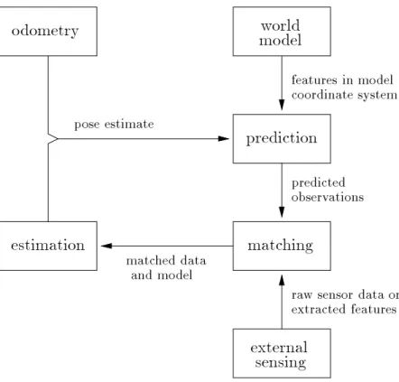
A typical pose estimation procedure is shown in Figure 2.1. In this procedure, rst a pose estimate is obtained from odometry. The world model, together with the pose estimate, provides prediction about the current sensor observation. After taking the sensor measurements, the cor-respondence between the sensor data and the predicted part of the model is determined, and any discrepancy between each corresponding data-model pair is used to correct the estimate of the robot pose. The major issues of this procedure are discussed below.

Sensing and feature extraction

The commonly used sensing methods are vision and range sensing. Vision is the most exible sensing technique. Although it only provides 2D images, various information such as depth, shape, motion can be extracted indirectly. The computer vision community has extensively studied these problems 43, 56, 64]. To interpret the image data for pose estimation, usually features are rst

(23)

estimation

odometry

observations

raw sensor data or extracted features and model matched data predicted

matching

model

world

pose estimate

prediction

sensing

external

features in model coordinate system

Figure 2.1: A typical procedure of pose estimation using both odometry and external sensing. First a pose estimate is obtained from odometry. The world model, together with the pose estimate, provides prediction about the current sensor observation. After taking the sensor measurements, the correspondence between the sensor data and the predicted part of the model is determined, and any discrepancy between each corresponding data-model pair is used to correct the estimate of the robot pose.

(24)

2.2. MATCHINGSENSOR DATA FOR POSE ESTIMATION 16

extracted. A widely used example drawn from image processing is the so-called \edge", which is some curve in an image in which a rapid intensity change occurs. Such a feature is hypothesized to correspond to some three-dimensional entity, either a change in reectance or a change in the surface structure. A potential problem is that feature detectors may be unreliable, and erroneous features lead to errors in pose estimation.

For robot pose estimation, range information is particularly useful and convenient to process. Commonly used range sensors include sonar and laser range-nder. Sonar is inexpensive, but its measurements are very noisy due to its wide beam width and specular reection. Laser range-nder gives more accurate readings and its range of measurements is also larger. Typically, a single shot of a range sensor gives one depth measurement. The sensor is thus often rotated in order to take a scan or an image of measurements which gives more context of the shape of the current environment. From a scan of range data, geometric features can be extracted for matching and recognition. The commonly used features are line segments, corners, depth continuities, curvature extrema, etc.. Geometric features are relatively more stable than image features. But due to occlusion, sensor noise, and pose uncertainty, these features are still dicult to interpret.

World model for pose estimation

A metric a priori world model provides the reference for pose estimation. The model keeps the geometric or other properties of features for recognition and the global coordinates of the features. If an estimate of the current pose is available, predictions about the current visible features can be made (i.e. to select the relevant features from the model). We will discuss in more detail about world models in a later section.

Matching and estimation

Matching is a procedure of associating features from sensing data with the model. With the feature-model correspondence, the current robot pose can estimated. We discuss the matching techniques in the following section.

2.2 Matching Sensor Data for Pose Estimation

The central issue in robot pose estimation is to match sensor data to a world model so as to infer the robot pose. Suppose that there is an error in the robot pose in the sense that the robot mistakenly thinks it is at one place while it is actually somewhere else. This pose error may lead to a discrepancy between the location of a data feature in a sensor coordinate system and the location

(25)

of the corresponding model of that feature (assuming a known model). By comparing the sensor data with the model, the robot can solve or correct its pose based on this discrepancy.

There are two issues involved in the matching techniques: nding the correspondence between the data and the model, and solving for the robot pose using the correspondence. The two issues are closely related to each other as one can usually be easily solved assuming the other. We discuss some matching techniques for pose estimation as the following.

2.2.1 Correlation Methods

Images (of either intensity or range) can be matched to another image by a correlation-based approach. Here one image (or a small region in the image) is placed in all possible relative positions and orientations with respect to the other image. Then one particular transformation between the two images which minimizes some sort of distance measure is selected as the matching solution. In robot navigation applications, correlation method is often used for matching grid-type world representations. For example, Elfes used a heuristically improved correlation method to match sonar maps which are represented in occupancy grids 42]. Correlating two grids usually takes extensive computation, especially when the grids are at dierent orientation.

Weiss et al used a correlation method to match range scans for keeping track robot position and orientation. They rst correlate the \angle histograms" of two scans to recover the relative orientation. Then the X and Y histograms are used to compute translation.

Straightforward correlation-based matching methods are generally unable to handle outliers. For example, if some areas are visible in one scan but not in the other because of occlusion, the correlation of the two scan may produce arbitrarily bad estimation. Robust techniques which limit the inuence of outliers have also been studied 13].

2.2.2 Combinatorial Search

Many matching techniques are feature-based. The typical process is to rst identify a set of features in the sensor data that potentially corresponds to entities in the world, and then match the features to a world model through some form of combinatorial search. In order to limit the exponential explosion in search complexity, various constraints and heuristics are applied.

In a vision-based robot navigation system, Fennema et al used a heuristic search technique coupled with an objective function to match image features to a known model 44]. The features used in their approach are the 2D line segments extracted from intensity images. The objective

(26)

function is dened on each possible state of correspondence between the lines in data and lines in the model, by taking into account both the tting error for the matched data-model pairs and the penalty for the unmatched model parts. The search strategy is to add or delete

k

lines from the data-model correspondence at every step, and try to search for a state with the minimum matching error. Once the correspondence is determined, the 3D camera pose is solved by a least-squares spatial tting procedure.

The above approach is very computationally expensive. An example in the paper shows that it can take hours to perform the model matching if the search is not focussed. Many issues still need to be addressed. Such as how to determine a good starting correspondence how to select

k

lines to add/delete etc.. The value of

k

also plays an important role in the method. Small

k

(such as

k

= 1) may leads to local minima in the evaluation function. For a larger value of

k

, the search space increases by

O

(

N

k_{) where}

_N

_{is the number of possible pairings of model and data lines.}

In addition to the high computational complexity in feature-based matching technique, another major problem is that the quality of matching depends on the reliability of features.

2.2.3 Statistical Data Association and Estimation

Probablistic models have been used to represent measurements with uncertainty. Typically, a measurement is modeled as a random variable with assumed Gaussian distribution. Uncertainty is then represented by the variance of the random variable.

Given a pose estimate, data-model correspondence can be determined by associating each fea-ture with the closest model. Besides, a threshold on the condence of matching can be set based on the pose uncertainty. If a feature is too far away from the closest model (exceeding the statistical threshold), it can be rejected as an outlier. An extensive study about statistical data association can be found in 9].

A dicult decision in data association is that, if more than one feature is within the acceptance zone of a model, which one(s) should be selected? Possible strategies include selecting the closest one, selecting the average of all close ones, or not to select any feature at all in case of ambiguity. Each strategy has its own drawbacks.

In the work by Leonard and Durrant-Whyte 78], geometric features called \regions of constant depth" are extracted from a scan of sonar range data. On the other hand, predictions about possible feature occurrences are generated based on a model and an estimate of the sensor pose. Sensing errors and positional errors are modeled as additive Gaussian random noises with known

(27)

covariances. A statistical test that measures the dierence between observation and prediction is applied to every pair of feature and model. Pairs satisfying the test are accepted as good matches. Other features that do not correspond to any model are discarded as outliers. A potential problem with this approach is that it relies on the reliable extraction of robust features from sonar data. But sonar data are usually very noisy and it might be dicult to obtain enough reliable features.

To register line segments extracted from images to model, Ayache and Faugeras also used probabilistic predictions of feature locations and their uncertainties 7]. To further improve the reliability of feature association, they employed a strategy which starts with registering features which have a small error covariance, or features which can be matched unambiguously. Uncertainty in the positions of the remaining features may be reduced when the robot's pose is updated using the good matching pairs. Then these remaining features can be registered more reliably.

Kosaka and Kak applied a more sophisticated procedure to probabilistically associate features to models based on a maximum likelihood criterion for the mapping function 69]. For each model element, the candidates of corresponding feature are the ones within the uncertainty region. The procedure sequentially selects trial model-feature correspondences and updates the robot pose using a Kalman lter. The optimal mapping is considered as a path in the correspondence search space which contains the minimum number of missing features and a maximum value for the objective function. Here the objective function is dened from the distances in the selected correspondence pairs, taking into account the sequential updates to the pose from previously selected correspon-dences along the current path. Backtracking is needed to select the optimal mapping function.

To avoid making irreversible decisions about data association at too early a stage, Cox and Leonard used a multiple hypothesis approach 32] which maintains more than one interpretation of sensor measurements at one time and carries these hypotheses over time. Thus ambiguity in data association in one step can be possibly resolved in a later step when more evidence is gathered.

Once the correspondence of features are determined, the next issue is to solve for or update the pose estimate using the correspondences. The Kalman lter and the extended Kalman lter are the most commonly used estimation algorithms. The linear Kalman lter gives an optimal estimate in the sense of least-squares or minimum variance. The extended Kalman lter linearizes a non-linear problem and then applies the non-linear Kalman lter 49, 90]. Many mobile robot navigation systems apply the (extended) Kalman lter for robot pose estimation and model construction (e.g. 7, 70, 34, 78]).

(28)

matrices. The sensor observation is modeled as

z

=

Hx

+

w

where

x

is the parameter to be estimated, usually the robot's pose

z

is the sensor observation reading

w

is the random sensor noise modeled as white Gaussian

H

is a linear transformation. The recursive Kalman lter gives the new estimate of

x

as:

x

=

x

0+

K

(

z

;

Hx

0)

K

=

S

0

H

T(

W

+

HS

0

H

T);1

S

= (

I

;

KH

)

S

0

W

=

E

ww

T_]

where

x

and

S

are the mean value and covariance matrix of the new estimate of

x

0 and

S

0 are

the previous mean value and covariance matrix of

x

.

Straightforward correction to robot pose (non-statistical) has also been employed in navigation systems. For example, in 33], the average angle between data and model line segments are used to x the robot's orientation, and the average displacement between data and model are used to correct the robot position. Spatial tting methods based on least-squares tting error are also used to solve for robot pose. These methods are often applied iteratively. We will study them in the next subsection.

2.2.4 Iterative Optimization Methods

The process of assigning correspondence and solving pose estimates can be carried out iteratively. In each cycle, a previous pose estimate is used to associate correspondences of data features to the model (assigning features to the closest model or using a statistical test). The correspondence pairs can be used to derive a potentially more accurate pose estimate (typically using a least-squares spatial tting method). The process repeats until the pose solution converges.

Cox et al proposed an iterative matching algorithm which uses range measurements directly as features (thus avoiding feature extraction) 31, 28, 29]. In their approach, the model consists of line segments of a world contour, while the data are the points on the world boundary received from a laser range-nder. The system maintains an estimate of the robot's pose, so the data points can be placed near the linear world model. Matching is accomplished by associating each point with its closest line segment in the model. A point may be regarded as outlier if it is too far away from

(29)

the model. Once the correspondences are determined, a least-squares tting is constructed as the following: Each data point is transformed with an undetermined congruence consisting of a rotation angle

and translation vector

t

. For each data point

v

i and the corresponding line model

m

i, a

tting error as a function of

and

t

is dened by summing up the distances from the transformed point

R

(

)

v

i+

t

to the line

m

i. Then the congruence is solved by minimizing the tting error.

The entire process of associating correspondence and tting is iterated until convergence. Finally, the derived congruence is applied to correct the robot pose.

Cox's method is ecient and eective for indoor linear environments (i.e. whose contours consist of mostly long line segments). The algorithm has the nice property that it does not require feature extraction, while it can also handle outliers to some extent. A limitation of the method is that it requires an analytical world model. Thus the method can not be directly applied for navigation in unknown environments. We are able to extend this algorithm, however, for matching a set of data points against another set of data by rst tting line segments to one set of data (see Chapter 5). In the CMU Navlab project, Hebert et al described a gradient descent optimization algorithm for matching terrain elevation maps 53]. The purpose of matching is to align the local maps so as to integrate them into a global map. The displacement (and correspondence) between two maps is determined by an unknown transformation

v

. A distance function

E

is dened as the sum of the squared distances between the corresponding points in the two maps. The function is then minimized with respect to

v

using an iterative gradient descent of the form:

v

i+1 ₌

_v

i₊

_k

@E

@v(

v

i).

The derivatives needed in the algorithm involve the gradient of the terrain surfaces which are computed from the maps. The algorithm requires an initial estimate of

v

to start the iteration.

2.2.5 Our Work

We take an approach to the robot self-localization problem that aligns laser range scans, similar to the approach of Cox et al. However, we consider more general cases as (1) an arbitrary two-dimensional world, not necessarily polygonal and (2) an unknown environment. We intend to address the localization problem for both path execution and exploration of unknown world. Since an analytical model of the environment is not available to us, we have to match a range scan to another reference scan in order to derive relative robot pose. This is much harder than matching data points to a linear world model.

In Part II of the thesis, we present two algorithms for aligning a pair of range scans. These algo-rithms use iterative optimization techniques and they do not require explicit feature interpretation.

(30)

2.3. WORLD MODELSFOR ROBOT NAVIGATION 22

The rst algorithm is based on a combined search/least-squares procedure to minimize a distance function and solve for the relative transformation between the scan poses, where the distance func-tion is dened from the approximated tangent lines at pairs of corresponding points on the two scans. The second algorithm is based on iteratively associating point-to-point correspondences and solving incremental updates to the transformation.

2.3 World Models for Robot Navigation

We rst discuss several types of a priori world models which are commonly used in navigation systems. Then we discuss the dynamic construction of models from sensing data. Finally, the issue of consistent data registration in dynamic model building is studied.

2.3.1 Types of World Model

A world model, also called a map, is an internal representation of the geometric, topological, or physical properties of the world. Major uses of a model include path planning and pose estimation. We are primarily interested in world models for pose estimation.

For the purpose of pose estimation, the world model should keep two types of information: the metric locations of the world entities and the descriptions of their features. The locations, usually represented by coordinates in a global reference frame, serve as the reference for computing vehicle pose. The descriptions are about the geometric or other types of distinct features that can be detected by sensors in order to recognize the entities. For primitive features, such as lines and points in images, the descriptions are often implicitly embedded in the recognition algorithm.

If there are xed, easily detectable beacons in the environment, then the world representation for robot self-localization may be simply a map recording the locations of these beacon. Many robot systems for industrial environments, such as AGV's (automated guided vehicles), use this approach. However, installing the beacons means altering the environment, which is only practical in very restricted domains. For more exible autonomous robot applications, natural features should be used.

A 2D contour model represents the boundaries of the objects (or free space) in the world as projected to the oor plane. The contour curve can be represented as a set of line segments (such as in 29, 33, 34]), by a parametric curve (e.g. using the curvature primal sketch 45]), or by features of the contour such as corners or occlusion boundaries 77, 78]. We also treat a set of points on the contour as a model for matching with another set of points (see Chapter 3). Typically, the

(31)

contour model is used for matching with range data or with features that have been extracted from range data. It appears that the contour model is adequate for navigation in a structured environment (e.g. a simple indoor environment) and the construction of such a model is relatively straightforward. However, since the model only represents geometric information and only in 2D space, it may be unable to model more complicated environments.

Occupancy grid is a simple representation scheme suitable for modeling an environment from range measurements 102]. This type of model represents a tessellation of the environment in 2D or 3D grids, while each elemental cell in the grid identies the state of a specic position as being \free space" or \obstacle". Sometime, the condence about whether a cell is occupied is also maintained. Because of its simplicity, a grid model is chosen in some navigation systems (e.g. 2, 94]).

Another type of model working with image data is the 3D CAD model 44]. It represents the 3D line segments in the scene which can be detected in intensity images. Line segments in the image are extracted as features to be matched with the model. The model is quite exible in modeling various kinds of environments, and the represented 3D structures are more informative for navigation than the contour model. However, if the world contains many curves, it would be inconvenient to model the world with line segments. Building such a detailed 3D model is usually a tedious task, in many situations even unrealistic. If the CAD model is used, the related feature matching problem can be very computationally expensive.

For robot exploration and mapping in large-scale spatial environments, qualitative and topo-logical models have also been suggested 71, 79, 37].

2.3.2 Dynamic World Modeling

The goal of dynamic world modeling is to acquire and represent geometric information about the environment automatically by the robot to facilitate navigation and other tasks. Here the word \dynamic" emphasizes that the world representation (model) is built or updated dynamically with successive readings of sensor data as the robot explores the world.

Dynamic world modeling is involved in mobile robot navigation in an unknown (or partially unknown) environment. The robot cumulatively builds a world model from the sensor data as it moves around. The robot maintains the following information at each cycle of updating the model: (1) a current global world model representing the areas discovered so far (2) some knowledge about its own pose and (3) a robot-centered geometric model of the local environment perceived at the current pose. The dynamic modeling process is to match the local model with the current global

(32)

model and update the global model.

In an unknown environment, the robot has no absolute reference. The same sensor data must be used for both correcting the robot's pose and updating the world model. This has been remarked as \pulling yourself up by your bootstraps" 34]. However, it is only possible to do this provided there is a substantial overlap between the observed data and the current model. This overlap provides the basis for pose correction, while the new information is added to the model.

Ayache and Faugeras proposed ideas of representing and maintaining spatial relationships of geometric primitives which are recognized by the robot 7]. In their approach, successive frames of local descriptions are fused to form a more global, coherent, and accurate representation. First, local descriptions of the environment (points, lines, etc.) are extracted from images. A set of geometric relations between the primitives of two visual maps are dened, such as \identical", \contained", \parallel", and \orthogonal". The geometric relations are expressed as the constraints on the parameters of the primitives. These relations are searched for among all the primitives in two maps. Each pair of primitives is registered by computing a probabilistic distance measure and verifying an acceptance test. After registration, two primitives are combined to produce a better estimate of their parameters and reduce the uncertainty. The tool used for matching and updating is the extended Kalman lter. The geometric relations provide nice constraints for interpreting image features. However, it appears that accidental alignments may lead to many false alarms if some weak relationships (such as parallel) are searched for among all pairs of primitives. There is another problem unsolved in this approach: When the relations among the primitives are detected, how can these relations be maintained systematically and consistently as more and more image data are acquired?

Kriegman et al 70] discuss the problem of exploring the free space for a mobile robot operating in an unknown indoor environment using stereo vision. A model of world contour is constructed and maintained by connecting all the observed feature points on the contour without violating the visibility constraints. At each step of sensing, feature points are extracted from stereo images and the points are matched to the existing ones in the model. Those points with correspondence in the model can help reducing the uncertainty in the model. Otherwise new points are inserted in the model to augment the discovered free space. An

O

(

n

3_{) algorithm is used to update the model while}

abiding the visibility constraints. A more ecient algorithm (

O

(

n

log

n

) time) for connecting the contour points without violating the visibility constraints is available 1]. The algorithm requires that all the points belong to a single simple object.

(33)

In 74], the problem of matching a local model with a global model and constructing a new global model is studied using simulated data. From each scan of range data, line segments are extracted and classied according to the status of how it is being occluded (for example, a line segment labeled as \left partial wall" means that the right end of the line is an occlusion boundary). The lines are matched to a global model with the constraints according to the line types and their poses. The matching process starts with a initial matching of complete walls and then propagates to the entire model. After a successful matching, several rules are applied to update the global model. The constructed model is globally consistent, which is desirable for global navigation. However, the weakness of this work is that sensing and line extraction are assumed to be perfect, which is quite impractical in real applications. Moreover, the approach did not make use of the robot's pose in registering local models onto the global model. Instead, a (constrained) global search is used to match models elements, which is quite inecient.

Crowley discussed the approach of building and maintaining a composite local model 33, 34] which is an intermediate level of representation of the environment in between a global model and a sensor model. The composite local model reects the immediate state of the local environment and it is used for local navigation. The model is built up by integrating recent information from sensors, taken from dierent poses, and also information from a pre-learned global model. The primitives of the composite local model are the line segments extracted from ultrasonic range data, representing the horizontal boundary of the world free space. Condence measures or probabilistic uncertainties of model primitives are maintained. Matching a pair of line segments is accomplished by a sequence of tests on the dierence in orientations, co-linearity, and overlap, with respect to the standard deviations of the uncertainties. With a successful matching, model parameters, as well as the estimated pose of the robot, are updated using the Kalman lter. In this system, the line segments in the model are maintained and updated independently from each other. The model can be inconsistent after several steps of updating. The approach must assume a linear world and require segmenting the range data into lines. Some similar approaches to constructing a world model consisting of line segments using sonar or laser sensing are reported in 38, 50].

The occupancy grid model is also used for representing an environment and integrating sensor data 42, 94, 2, 35]. A grid model is useful when a geometric interpretation of data is dicult due to large amounts of sensory noise, such as in the case of sonar.

In order to model a 3D outdoor scene, elevation maps are typically used. Asada discussed a mapping system which extracts the heights of obstacles in the scene from range images and

(34)

correlates local maps to update a global map 5].

A method of continuously updating a map using range measurements by a neural network is discussed in 95]. Pose error in dierent sensor locations is not considered in this work. A study on models for cognative maps using neural networks with potential application for mobile robots is discussed in 99].

Dynamic construction of a topological model requires precise identication of landmarks or markers 37]. So far we have only seen theoretical work in this direction.

2.3.3 Consistency in Dynamic World Models

The general approach to dynamic world modeling is based on aligning successive frames of sensor data or aligning each local frame with a cumulative global model, and then integrating the new frame of data into the global model by averaging the data or using a Kalman lter. A major problem with this approach is that the resulting world model eventually becomes inconsistent as dierent parts of the model are updated independently. Moreover, even if some inconsistency in the model is detected in a later stage, it may not be resolved because the data in the model may have been permanently integrated.

Clearly, the problem is that new frames of data are irreversibly integrated into the global model at too early a stage. In order to avoid this problem, the local coordinate systems of the data frames must be maintained and there must be some mechanism to resolve the inconsistency among the data frames once such inconsistency is recognized.

Consider the following scenario. The model contains two frames of data which are associated with poses (or local coordinate systems)

P

1 and

P

2, respectively. Suppose that a new frame of

sensor data is collected at pose

P

3 and geometric relationships of both

P

3

P

1 and

P

3

P

2 are derived

from matching the frames of data (the relationships are illustrated in Fig. 2.2). Now if we register frame

P

3 to either frame

P

1 or

P

2, it may be inconsistent with the other frame because the three

relationships,

P

1

P

2,

P

3

P

1, and

P

3

P

2, could be inconsistent as they are derived from dierent sources.

Therefore, in order to register the new frame to the model, we should rst resolve the inconsistency among the three poses. Based on the three relationships and their uncertainties, we can update

P

1,

P

2, and

P

3 to make them consistent (i.e. to ensure that the composition of

P

1

P

2,

P

2

P

3 and

P

3

P

1 yields an identity transformation). Generally, if there are other frames of data in the model

which are related to

P

1and

P

2, they should also be updated at the same time to ensure consistency

(35)

current model

P

2

P

1

P

3

new frame of data

Figure 2.2: Illustration of relationships between model and new data.

Chatila and Laumond studied the consistency issue in dynamic world modeling in their HILARE robot project 25]. In their system, range signals are segmented into objects and each discovered object is associated with a local object frame. The local frame itself is referenced in an absolute global frame along with the uncertainty on the robot's pose at which the object frame is constructed. New sensor data are matched to the current model of individual object frames. If some object which has been discovered earlier is seen again, its object frame pose is updated (by averaging). In circumstances that the uncertainty of some object frame in the model is less than the uncertainty of the current robot pose (note: this happens when the object frame is created earlier, and later the robot sees the object again), the robot's pose may be corrected with respect to that object frame. After correcting the current robot pose, the correction is propagated backwards with a \fading" eect to correct the previous poses. The object frames created at these poses can also be updated. Although the HILARE system considered the issue of resolving model inconsistency, the solution does not appear to be satisfactory in the following aspects. First of all, the system associates local frames with \objects". But if the results of segmenting sensor data or matching the data with model are imperfect, the \objects" and therefore the local frames may not be dened or maintained consistently. When a previously recorded object is detected again, the system only attempts to update the poses (and the associated frames) along the path between the two instances of detecting this object, while the global consistency among all frames in the model may not be maintained. HILARE only uses a scalar random variable to represent the uncertainty of a three-degree-of-freedom pose, which seems inadequate. Using a heuristic \fading" function to determine the updates to the poses also appears to be inadequate. A statistical lter may be applied here.

SHAPE REGISTRATION USING OPTIMIZATION FOR MOBILE ROBOT NAVIGATION. Feng Lu

SHAPE REGISTRATION USING OPTIMIZATION

FOR MOBILE ROBOT NAVIGATION

by

Feng Lu

A thesis submitted in conformity with the requirements

for the degree of Doctor of Philosophy

Graduate Department of Computer Science

University of Toronto

c

Shape Registration Using Optimization

For Mobile Robot Navigation

Abstract

Acknowledgements

Contents

1 Introduction

1

: : : : : : : : : : : : : : : : : : : : : : : : : : : : : : : : : : : : :

: : : : : : : : : : : : : : : : : : : : : : : : : : : :

: : : : : : : : : : : : : : : : : : : : : : : : : : : : : : : : :

: : : : : : : : : : : : : : : : : : : : : : : : : : : : : :

: : : : : : : : : : : : : : : : : : : :

: : : : : : : : : : : : : : : : : : : : : : : : : : : : : : : : : : : : : : :

I Review of Related Work

8

2 Review of Related Work

10

: : : : : : : : : : : : : : : : : : : : : : : : : : : : : : : : :

: : : : : : : : : : : : : : : : : : : : : : : : : : : :

: : : : : : : : : : : : : : : : : : : : : : : : : : : : : : : : : :

: : : : : : : : : : : : : : : : : : : : : : :

: : : : : : : : : : : : : : : : : : : : : : : : : : : : : : : :

: : : : : : : : : : : : : : : : : : : : : : : : : : : : : : :

: : : : : : : : : : : : : : : : : : :

: : : : : : : : : : : : : : : : : : : : : : : : :

: : : : : : : : : : : : : : : : : : : : : : : : : : : : : : : : : : : : : :

: : : : : : : : : : : : : : : : : : : : : : : : : : :

: : : : : : : : : : : : : : : : : : : : : : : : : : : : : : :

: : : : : : : : : : : : : : : : : : : : : : : : : : : : :

: : : : : : : : : : : : : : : : : : : : : :

: : : : : : : : : : : : : : : : : : : : : : : : : : : : : : : : : : : : : :

: : : : : : : : : : : : : : : : : : : : : : : : : : : : : : : : : : : : :

: : : : : : : : : : : : : : : : : : : : : : : : : : : : :

: : : : : : : : : : : : : : : : : : : : : : : : : : : : :

: : : : : : : : : : : : : : : : : : : : : : : : : : : :

: : : : : : : : : : : : : : : : : : : : : : : : : : : : : : : : : : : : : :

II Matching Range Scans for Robot Pose Estimation

35

3 A Search/Least-Squares Algorithm for Matching Scans

37

: : : : : : : : : : : : : : : : : : : : : : : : : : : : : : : : : : : : :

: : : : : : : : : : : : : : : : : : : : : : : :

: : : : : : : : : : : : : : : : : : : : : : : : : : :

: : : : : : : : : : : : : : : : : : : : : : :

: : : : : : : : : : : : : : : : : : : : : : : :

: : : : : : : : : : : : : : : : : : : : : : : : : : : : : : :

: : : : : : : : : : : : : : : : : : : : : : : : : : : : : : : : : : :

: : : : : : : : : : : : : : : : : : : : : : : : : : : : : : : :

: : : : : : : : : : : : : : : : : : : : : : : : : : : : : : : : : : :

: : : : : : : : : : : : : : : : : : : : : : : : : : : : : : : : : : : : : : : :

: : : : : : : : : : : : : : : : : : : : : : : : : : : : : : : : : : : : : : : : : :

4 Point Correspondence Based Matching Algorithm

50

: : : : : : : : : : : : : : : : : : : : : : : : : : : : : : : : : : : : :

: : : : : : : : : : : : : : : : : : : : : : : : : : : : : : : : :

: : : : : : : : : : : : : : : : : : : : : : : : : : : : : : : : :

: : : : : : : : : : : : : : : : : : : : : : : : : : : :

: : : : : : : : : : : : : : : : : : : : : : : : : : : : :

: : : : : : : : : : : : : : : : : : : : : : : : : : : : : : : : : : : : : : :

: : : : : : : : : : : : : : : : : : : : : : : : : : : : : : : : : : : : :

: : : : : : : : : : : : : : : : : : : : : : : : : : : :

: : : : : : : : : : : : : : : : : : : : : : : : : : : : : : : : : : : : : : : : : :

5 Scan Matching Experiments

59

: : : : : : : : : : : : : : : : : : : : : : : : : : : : :

: : : : : : : : : : : : : : : : : : : : : : : : : : : : : : : : : : : : : :

: : : : : : : : : : : : : : : : : : : : : : : : : : : :

: : : : : : : : : : : : : : : : : : : : : : : : : : : : : : :

: : : : : : : : : : : : : : : : : : : : : : :

: : : : : : : : : : : : : : : : : : : : : : : : : :