REPRESENTATION LEARNING ON SEQUENTIAL
MEDICAL DATA
A Dissertation
Presented to the Faculty of the Weill Cornell Graduate School of Medical Sciences
in Partial Fulfillment of the Requirements for the Degree of Doctor of Philosophy
by
Stephanie L. Hyland May 2019
c
2019 Stephanie L. Hyland ALL RIGHTS RESERVED
REPRESENTATION LEARNING ON SEQUENTIAL MEDICAL DATA Stephanie L. Hyland, Ph.D.
Cornell University 2019
The way we do medicine is undergoing a revolution driven by technology. As the modern drive to record, share, and analyse data sweeps across soci-ety, healthcare lies squarely in its path. Data generated by every-day clinical practice presents an invaluable view of health and disease at a scale previously unimaginable. However, to benefit from it, we need computational tools to ex-tract meaning, clinical insight, and actionable predictions. This new digital era of medicine is an opportunity not only for healthcare providers, but also for machine learning researchers to develop new methods tailored to the unique demands of this complex domain. The work described here sits in this sphere.
Firstly, we explore representation learning for medical language. With its long-tailed distribution of technical terms, medical language necessitates devel-opment of methods to augment data-scarcity by exploiting prior information encoded in knowledge graphs. Obtaining semantically meaningful represen-tations of medical concepts and their relationships is vital, and we describe a probabilistic model to learn such representations.
Secondly, we address learning from long time series using recurrent neural networks. These long sequences are commonplace in medicine, where one’s health history is necessarily lengthy, but early events nonetheless provide cru-cial context. To address vanishing and exploding gradients in the training these networks, we propose a novel parametrisation exploiting the correspondence between the Lie group of unitary matrices and its Lie algebra.
Next, a method for generating synthetic ICU time series data is described in the framework of adversarial networks. A core challenge for researchers in healthcare is the scarcity of shareable datasets on which to benchmark. Realistic synthetic data is therefore key. Novel methods for evaluating the quality of this synthetic data are proposed, and the model’s privacy and memorisation properties are analysed, both heuristically and in terms of differential privacy.
Finally, an ensemble of gradient-boosted decision trees are employed to identify circulatory system deterioration in Swiss ICU patients. As this sys-tem has been developed for deployment, we carefully detail the data process-ing steps, task specification, and evaluation considerations necessary for a real-world, real-time early warning system driven by machine learning.
BIOGRAPHICAL SKETCH
Stephanie L. Hyland is from Dublin, Ireland. She studied Theoretical Physics at Trinity College Dublin between 2008 and 2012, where she was awarded a BA(Mod.). She then undertook Part III of the Mathematical Tripos at Cambridge University, where she studied Theoretical Physics and Applied Mathematics. During this time, while supported by the Bill and Melinda Gates Foundation, she started to seek research directions outside of theoretical physics, looking for a way to have more immediate impact on society. The conclusion of this delib-eration was the decision to travel to the USA in 2013 to join the Tri-Institutional Training Program in Computational Biology and Medicine at Cornell Univer-sity, Weill Cornell Medical, and Memorial Sloan Kettering Cancer Center. Here, she learned about how machine learning could be used for problems in funda-mental biology and medicine, and how physics and mathematics could be used for problems in machine learning. In 2014 she moved from Cornell’s home town of Ithaca to its medical campus in New York City, where she joined the group of Gunnar R¨atsch, who would become her supervisor. In 2016 the R¨atschlab moved to ETH Z ¨urich, and so she returned to her home of Europe to complete her PhD studies, retaining her affiliation with the CBM program.
ACKNOWLEDGEMENTS
This would have not been possible without the support of my adviser Gunnar R¨atsch, who afforded me the freedom to develop as a scientist, and who be-lieved in me when I didn’t believe in myself.
I would like to express my gratitude to my examination committee for their guidance, wisdom, and patience, especially reading the next several hundred pages. They are Adam Siepel, Olivier Elemento, and Thomas Fuchs.
Throughout these years I have had colleagues in New York and Z ¨urich, and who collectively create the welcoming and open atmosphere of the R¨atschlab. Through our discussions over lunch, in lab meetings, at conferences and re-treats, I have learned from you all and grown both as a scientist and as a person.
In particular, I would like to thank:
Theofanis Karaletsos for many discussions on life, the universe, and modelling, Matthias H ¨user and Xinrui Lyu for putting up with me,
Stefan Stark and David Kuo for their mastery of mythology and sports trivia, Andre Kahles and Kjong Lehmann for sagely wisdom,
Crist ´obal Esteban for understanding the struggle, Francesco Locatello for giving me new perspectives,
Melanie Fernandez Pradier for lessons on work-life balance, Martin Faltys for giving me the clinical side of the story,
and everyone else over the years, in the R¨atschlab, Memorial Sloan Kettering Cancer Center, and the Institute for Machine Learning at ETH Zurich.
Outside of the R¨atschlab, I have also been fortunate to benefit from the inim-itable positivity of Charles Danko, and the guidance and wisdom of Danielle
Belgrave. I must also acknowledge my godmother Jennifer Pearson, the first person I met with a PhD, who made it look far too easy.
I would like to acknowledge the Tri-Institutional PhD Program in Compu-tational Biology and Medicine, which started the whole affair of having confus-ingly many affiliations.
Crossing the Atlantic to live in a foreign land would have been a lot lonelier without evenings on the balcony at Coddington with Noah Dukler, Nate Tip-pins, Mary Centralla, Ozan Sener, Aditya Vaidyanathan, and everyone else in Ithaca.
Margie Hinonangan-Mendoza, Kadeem Ho Sang, Sabrina Nepozitek, and Natalia Marciniak went beyond the call of duty to smooth the complexities of doing a PhD across two continents.
Science cannot be done in an vacuum, and I am extremely grateful for the support of my friends over the last five years. You all brought me back to earth when I got carried away, and lifted my spirits in heavy moments.
In particular I am deeply indebted to the friendship of:
Jennifer Lorigan, who has always been there, and I hope always will be, Neel S. Madhukar, whose exuberance and sincerity I shall always admire, Natalie Davidson for her energetic creativity and kindness,
Faisal Alquaddoomi for his insightful and caring nature,
Cian Booth for his lightheartedness and for forcing me to take breaks, Fionn Fitzmaurice for personifying freedom,
Regina Kelly and Ruairi Short for knowing what it’s like to emigrate,
Matthew Carrigan for reminding me that not everything has to be rigorous, but everything must be rational,
debate in a fragmenting world, Calvin Hu for liking all my tweets,
Zachary Elliott for patience during my second transatlantic voyage,
The members of NYC Resistor and New New York for giving me a third place for a while,
Z ¨urich City Roller Derby for teaching me to be strong, the rest of my friends scattered across the world, and Oli Stiel, for dreaming with me.
Finally, I am endlessly grateful to my family; my dog Yuki, my sister Jes-sica and her husband Alex for forgiving my absentmindedness, and my parents Mary Walsh and Keith Hyland, for being unconditionally supportive and un-derstanding.
TABLE OF CONTENTS
Biographical Sketch . . . iii
Dedication . . . iv
Acknowledgements . . . v
Table of Contents . . . viii
List of Tables . . . xi
List of Figures . . . xiii
1 Introduction 1 1.1 Motivation . . . 1
1.2 Structure of the dissertation . . . 3
2 Medical Text 6 2.1 Word representations . . . 8
2.1.1 Distributional semantics . . . 10
2.1.2 Latent semantic indexing . . . 12
2.1.3 Neural word embeddings . . . 14
2.1.4 Skip-gram and continuous-bag-of-words . . . 15
2.2 Representing facts . . . 19
2.2.1 Knowledge graphs . . . 20
2.2.2 Building and representing knowledge graphs . . . 21
2.2.3 Combining knowledge graphs with free text corpora . . . 26
2.3 Contributions . . . 27
2.3.1 Learning representations of words and relationships . . . 28
2.3.2 Relationships as context . . . 29
2.3.3 Probabilistic modelling . . . 30
2.4 Experiments and analyses . . . 35
2.4.1 Data . . . 36
2.4.2 Experimental details and implementation . . . 40
2.4.3 Triplet classification . . . 40
2.4.4 Embedding quality . . . 43
2.4.5 Extending a medical knowledge graph . . . 49
2.5 Conclusions and future work . . . 56
3 Long-Memory Recurrent Neural Networks 58 3.1 Background on long-memory RNNs . . . 60
3.1.1 Vanishing and exploding gradients . . . 61
3.1.2 Long short-term memory . . . 63
3.1.3 Orthogonal and unitary RNNs . . . 64
3.2 Parametrising a unitary RNN . . . 68
3.2.1 Lie groups and lie algebras . . . 68
3.2.2 Parametrization ofU(n)in terms ofu(n). . . 73
3.2.4 Derivative of the matrix exponential: details . . . 77
3.3 Supervised learning of unitary matrices . . . 81
3.3.1 Task . . . 82
3.3.2 Comparison of approaches . . . 84
3.3.3 Restricting to7nparameters . . . 85
3.3.4 Method of generatingU . . . 86
3.3.5 Changing the basis ofu(n) . . . 88
3.4 Unitary RNN for long memory tasks . . . 89
3.4.1 Adding problem . . . 91
3.4.2 Memory problem . . . 93
3.5 Conclusions and future work . . . 95
4 Synthesising Medical Data 97 4.1 Why synthesise medical data? . . . 97
4.1.1 Reproducibility in medical machine learning . . . 98
4.1.2 Benchmarks and competitions . . . 100
4.1.3 Synthetic data in machine learning and healthcare . . . 103
4.2 Contributions . . . 104
4.3 Generative adversarial networks . . . 104
4.3.1 Recurrent GANs . . . 106
4.3.2 Conditional GANs . . . 108
4.3.3 Generating realistic sequences with RCGAN . . . 111
4.4 Evaluation of generative models . . . 114
4.4.1 Existing evaluation methods for GANs . . . 115
4.4.2 Our task-based score . . . 122
4.4.3 Performance of RCGAN with TSTR . . . 124
4.5 Privacy implications . . . 128
4.5.1 Model memorisation . . . 128
4.5.2 Differentially private GAN training . . . 133
4.6 Conclusions and future work . . . 138
5 Modelling Intensive Care 139 5.1 The Intensive Care Unit . . . 140
5.1.1 Machine learning and the ICU . . . 140
5.2 Circulatory failure prediction . . . 142
5.2.1 Definition of circulatory system failure . . . 144
5.2.2 Definition of prediction task . . . 146
5.3 Data preparation and processing . . . 147
5.3.1 Data and patient filtering . . . 147
5.3.2 Converting drugs to flow rates . . . 149
5.3.3 Variable merging . . . 151
5.3.4 Imputation . . . 153
5.4 Modelling . . . 156
5.4.2 Model . . . 164
5.5 Experiments and results . . . 165
5.5.1 Experimental setup . . . 165
5.5.2 Choosing models . . . 167
5.5.3 Deterioration prediction . . . 170
5.5.4 How much lead-time does the model provide? . . . 172
5.5.5 How well does the model generalise in time? . . . 173
5.5.6 How well does the model generalise to a different ICU? . 175 5.5.7 Event-based evaluation . . . 179
5.6 Conclusions and future work . . . 183
LIST OF TABLES
3.1 Performance of different parametrisations in a supervised uni-tary matrix learning task. The table shows the mean l2-norm between yˆi andyi on the test set for the different approaches as
the dimension of the unitary matrix changes. truerefers to the matrix used to generate the data, projectionis the approach of ‘re-unitarising’ using a polar decomposition after gradient up-dates, arjovskyis the composition approach defined in Equa-tion 3.7,u(n)is our parametrization (Equation 3.15) andrandis a random unitary matrix generated in the same manner astrue. Values in bold are the best for thatn(excludingtrue). The error fortrueis typically very small, so we omit it. . . . 85 3.2 Impact of restricting the parametrisation. We observe that
re-stricting our approach to the same number of learnable parame-ters as that of Arjovsky and Shah (2015) causes a similar degra-dation in performance on the task. This indicates that the rel-atively superior performance of our model is explained by its generality in capturing arbitrary unitary matrices. . . 86 4.1 TSTR results for MNIST. Scores obtained by a convolutional
neural network when: a) trained and tested on real data, b) trained on real and tested on synthetic, and c) trained on syn-thetic and tested on real data. . . 125 4.2 TSTR results on eICU. Performance of random forest classifier
for eICU tasks when trained with real data and when trained with synthetic data (test set is real), including random predic-tion baselines. AUPRC stands for area under the precision-recall curve, and AUROC stands for area under ROC curve. Italics de-notes those tasks whose performance were optimised in cross-validation. SpO2 = oxygen saturation measured by pulse oxime-try; HR = heart rate; RR = respiratory rate; MAP = mean arterial pressure. . . 127 5.1 Definition of circulatory failure. The level of severity is set by
the strength of the vasoactive support given through drugs. . . . 144 5.2 Patient demographics. For length of stay, we do not consider
data from patients after their 28th day in the ICU (this applies to 137 patients only). We define length of stay as the time be-tween the first and last recorded heart rate measurement. Note that patients can have more than one APACHE diagnostic group. The ‘other’ category includes trauma, gastrointestinal, sepsis, metabolic, haematological, orthopaedic, gynaecological, and re-nal (all below 5%). . . 150
5.3 Examples of how the same variable is recorded in multiple ways. To reduce redundancy in our features and imputation needs, we merge these ‘duplicated’ variables. Note that ZVD is Zentraler Venendruck - central venous pressure. . . 151 5.4 Categorisation of variables by frequency and corresponding
window sizes. Each variable is categorised as high, medium, or low frequency based on its median sampling interval. Four win-dows are defined for each category in order to define multiscale features. . . 160 5.5 Top variables by mean absolute SHAP value. These top
variables, from the reference model are used to define the reducedmodel. A variable is ranked by its most important fea-ture, which is shown in the second column. ‘Vasoactive drugs’ means dobutamine, milrinone, levosimendan, theophyllin. These are all potentially used to identify level 1 circulatory dysfunction, hence appear as a group. . . 170 5.6 Performance of model in different temporal splits. We train
a model on the training set of each temporal split and use its validation set for model selection, then report its test set perfor-mance. AUPRC in different splits is not directly comparable due to differences in positive label prevalence. We do not observe an obvious trend in AUROC, indicating that the generalisation error of the model is not time-dependent. Using the ‘mixed’ split, whose test set is selected from the same temporal distri-bution as the training set, we see that the temporal stratification approach is necessary to avoid overestimating the performance of the model. Values in brackets denote uncertainty (standard deviation) in the final digit over the temporal splits. . . 174 5.7 Performance of a fixed model as the test set varies. We develop
a model on the earliest split and test it on the test sets of subse-quent splits, in order to assess if temporal distance results in a higher generalisation error. In the ‘ratio’ rows, we compare the performance in this setting with the results in Table 5.6, where the model would instead be retrained on more recent data. We don’t see an obvious downward trend in the model’s perfor-mance, indicating that dataset shift is not significant over a two-year period. . . 175
LIST OF FIGURES
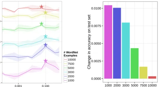
2.1 Unstructured data improves triplet classification. In addition to training on a set of known relationships, we use unstructured data from Wikipedia with varying weight (x-axis) during train-ing. As before, with the goal to predict if a triple(S, R, T)is true by using its energy as a score. A validation set is used to deter-mine the threshold below which a triple is considered ‘true’. The solid line denotes the average of three independent experimen-tal runs; shaded areas show the range of results. The bar plot on the right shows the difference in accuracy betweenκ= 0and κ = κ∗, whereκ∗ gave the highest accuracy on a validation set. Significance at 5% (paired t-test) is marked by an asterisk. We find then that unstructured Wikipedia can improve relationship learning in cases when labelled relationship data is scarce. . . . 43 2.2 Relationship data improves learned embeddings. We apply
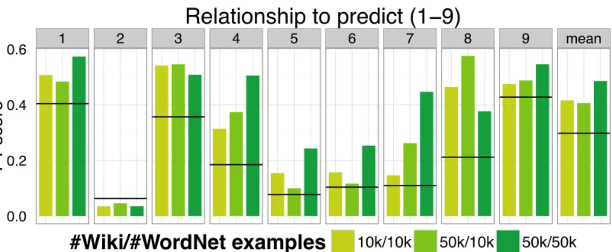
our algorithm on a scarce set of Wikipedia co-occurrences (10k and 50k instances) with varying amounts of additional, unre-lated relationship data (10k and 50k relations from WordNet). We test the quality of the embedding by measuring the accu-racy on a task related to nine relationships (see text for which). In each case, we used eight of the relationships together with the Wikipedia data to learn representations that are then used in a subsequent supervised learning task to predict the remaining ninth relationship based on the representations using random forests. Black lines denote results from word2vectrained on a Wikipedia-only with 4,145,372sentences. . . 46 2.3 Unsupervised learning of latent relationships improves
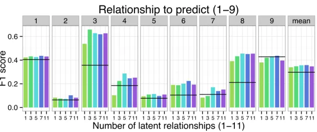
em-beddings. We train a fully unsupervised algorithm with 1, 3, 5, 7 and 11 possible latent relationships on one million Wikipedia sentences. Initialisation is at random. To test the quality of the resulting embeddings, we use supervised learning of nine Word-Net relationships with random forests. Depending on the rela-tionship at hand, the use of multiple latent relarela-tionships during training leads to slightly, but consistently better accuracies us-ing the computed embeddus-ings for every of the nine relationships and also on average. Hence, the resulting embeddings using la-tent relationships can be said to be of higher quality. Once again, black lines show results usingword2vec. . . 49
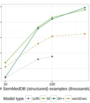
2.4 Predicting the relationship between concepts. With more struc-tured data, the model can better predict the correct relationship for a given (S, T) pair. bf++ has an additional 100,000 triples from EHR: with little structured data, so much off-task informa-tion is harmful, but provides some benefit when there is enough signal from the knowledge graph. Baselines are a random for-est taking [f(S) :f(T)]as an input to predict the labelR, where the feature representationf is either a 1-hot encoding (1ofN) or 200-dimensional word2vec vectors trained on PubMed. 1ofN proved too computationally expensive for large data. . . 51 2.5 Probability mass assigned to correct answers in the
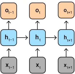
knowl-edge graph completion and knowlknowl-edge transfer task. The right column shows results for test triples where at least one of S and T is foundonly inEHR, and therefore represents the knowl-edge transfer setting. Information about relationships found in SemMedDB must be transferred through the joint embedding to enable these predictions. Grey dotted lines represent a random-guessing baseline. . . 54 3.1 Schematic of a recurrent neural network.The hidden statehtof
the network at timetdepends on the previous hidden state (ht−1) and the observed data (xt). The model can produce outputs ot,
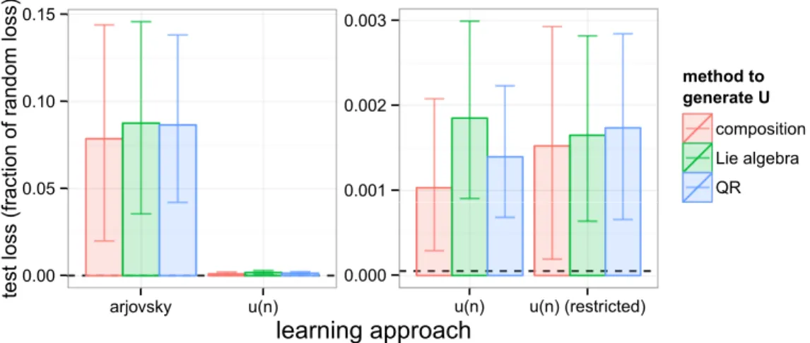
such as predictions, at each time step. . . 59 3.2 Impact of method of generating the unitary matrix. We ask
whether the method used to generateU influences performance for different approaches to learningU. Error bars are bootstrap estimates of 95% confidence intervals. To compare across differ-ent n’s, we normalise each loss by the loss of rand for that n, and report fractions. The dotted line is thetrue loss, similarly normalised. the choice of method to generateU does not appear to affect test-set loss for the different approaches. Right: Finer resolution on the u(n) result in left panel. We also include the case where we restrict to7nlearnable parameters. . . 87
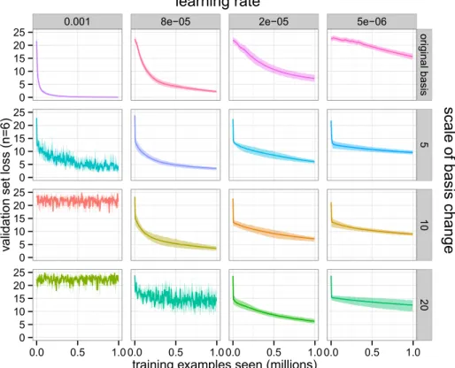
3.3 Impact of changing the basis of the Lie algebra. We consider the effects on learning of changing the basis (rows) and chang-ing the learnchang-ing rate (columns). For this experiment,n = 6. The first row uses the original basis. Other rows use change of basis matrices sampled fromU(−c, c)wherec={5,10,20}. The learn-ing rates decrease from the ‘default’ value of 0.001 used in the other experiments. Subsequent values are given by 0.c0012 for the above values of c, in an attempt to rescale by the expected ab-solute value of components of the change of basis matrix. If the change of scale were solely responsible for the change in learning behaviour, we would therefore expect the graphs on the diago-nal to look the same. . . 90 3.4 An example of the adding problem. The RNN receives a
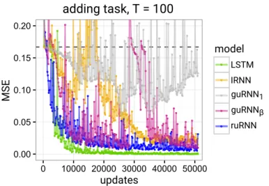
2-dimensional input sequence of length T (large). The second, bi-nary dimension of the input indicates which entries should be added (highlighted in red).Note that in practice, the first dimen-sion contains real values in[0,1]and not integers as shown. . . . 92 3.5 Comparison of different long-memory RNN architectures on
the adding problem. Here T = 100. The scaling factor β in front ofU in guRNN is 1.4 to compensate for the tendency of the nonlinearity (relu) to shrink gradients. The dotted line denotes the random baseline value of 0.167. . . 93 3.6 An example of the memory problem. The RNN receives a
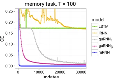
1-dimensional input sequence of lengthT (large) + 20. The first 10 entries are of interest, and are followed byT −1zeroes (‘blank’ token), then a single special token (shown as 9 in green), and 10 more zeroes. The special token indicates to the RNN that it should begin reproducing the memorised sequence. The RNN must then output T + 10zeroes followed by the sequence of in-terest. Performance is measured by cross-entropy between the full true and output sequences. . . 93 3.7 Comparison of different long-memory RNN architectures on
the memory problem. HereT = 100. The dotted line denotes the random baseline value of10 log(8)/(T + 20) = 0.173. . . 94 4.1 Schematic of the RCGAN architecture. . . . 110 4.2 Examples of real and generated samples of sine waves and
smooth signals.The top row shows real samples (in colour). The bottom two rows (in black) show generated samples. Smooth signals consist of samples from a Gaussian process with RBF ker-nel, evaluated at 30 equally-spaced points. . . 112
4.3 Examples of real and generated MNIST samples. Left top: real MNIST digits. Left bottom: unrealistic digits generated early in training. Right: digits with minimal distortion generated at epoch 100. . . 114 4.4 Learning curves, MMD score, and held-out log-likelihood for
RGAN generating smooth sequences. Trace of generator (dot-ted), discriminator (solid) loss, MMD2 score and log likelihood of generated samples under the data distribution during training for RGAN generating smooth sequences (output in Figure 4.2.) . 119 4.5 Assessing model memorisation using interpolation in latent
space. Here, we take two training examples (bottom and second-from-top plots, dashed green lines) and back-project them to find their closest points in latent space. We then linearly inter-polate these points and pass them through the generator, pro-ducing intermediate samples. These are shown in grey. The top graph shows the distance in sample space (using the RBF ker-nel) between the intermediate generated sample and both of the endpoints (respectively in green and orange). If model mem-orisation had occurred, we would expect the model to prefer-entially generate samples that look very similar to either of the endpoints, switching between these options perhaps half-way through. Instead, the generator produces samples which appear to vary smoothly as the latent point is varied. . . 132 4.6 Trade-off betweenandδ, and training epochs. Probability (δ)
of violating -differential privacy during training, for different values ofusing the moments accountant. Noise ∼ N(0,0.22)is used. The dotted line showsδ = 1/|D|, where|D|is the number of training examples. . . 136 4.7 TSTR results on four ICU prediction tasks. We compare data
generated by a non-private GAN (dark grey) and a GAN trained using differential privacy (light grey). The other three predic-tion tasks were used for model selecpredic-tion and are omitted here. We see that for some tasks, differentially private training of the GAN does not significantly impact the quality of the data mea-sured by TSTR, but overall there is, as expected, a performance degradation. Here,= 0.5withδ ≤0.9×10⁻³. Clipping was set toC = 0.1and the noise parameterσ = 2. . . 137 5.1 An illustration of noise in the signal from a pulse oximeter.
The noise results in an erroneous value of SpO2. Physiologi-cally implausible values such as 5% for SpO2 are removed dur-ing artefact removal. . . 148
5.2 Flowchart showing patient inclusion and exclusion steps. In the end, we use a set of 36098 patients to build and evaluate the predictive model. Of thee patients, 9801 have instances of circu-latory dysfunction. . . 148 5.3 A schematic showing how the same drug can be administered
through multiple delivery routes simultaneously. Most com-monly, a patient receives multiple infusions at the same time. For delivery routes such as injections and tablets, we convert the dose into an effective ‘rate’ by considering it to be delivered con-tinuously over a time period , which is defined for each drug based on clinical prior knowledge of its acting period. . . 151 5.4 A schematic depicting the imputation strategy for
time-varying variables. For each variable v, a timescale ∆v is
com-puted as the median of the variable’s sampling interval plus twice its interquartile range. Imputation then forward-fills for
∆v, before decaying over a time∆v to the median value over the
time-period 2∆v before the last observed measurement. After
that, indefinite forward filling is applied. . . 156 5.5 Feature classes extracted from time-series data. Using
overlap-ping windows of increasing size, we summarise the time series at multiple resolutions using 5-point summary statistics (mini-mum, maxi(mini-mum, median, interquartile range, trend). We record the time since the last non-imputed measurement, as well as statistics about the fraction of the patient’s time spent in endpoints.158 5.6 Change of RASS over time. The movement away from heavy
sedation in critical care is reflected in the Inselspital data. Values show the mean RASS (Richmond Agitation-Sedation Score) in each month. This highlights that, even within an 8-year period, the practice of critical care is not stationary. . . 165 5.7 Schematic showing how temporal splits are constructed. The
hatched region shows the validation set for a given split, and the coloured region is the test set. The same methodology is applied to each split - the validation and test sets comprise the patients in the final 20% of the split. Imputation parameters are computed on the training set, and the validation set is used for model se-lection. . . 166 5.8 Distribution of feature importances by class. Histogram of
(log) feature importances in the reference model computed using mean absolute SHAP value, broken down by feature class. Higher is more important. . . 168
5.9 Effect of removing different classes of features from the referencemodel. Note the small variation in the y-axis. This indicates that no one feature class contributes substantially more than others. However, it also indicates that there is redundancy between feature classes. . . 169 5.10 Performance of the models in predicting circulatory system
de-terioration in the next 8 hours. Receiver-operating characteris-tic and precision-recall curves for thereferenceandreduced models, which use 1000 features (on 198 variables) and 20 vari-ables respectively. The baseline prevalence of positive events is 3.8% over all timepoints. Results in this experiment are reported on the fifth (most recent) temporal split. The precision-recall curve demonstrates the trade-off between false alarms and sen-sitivity. At a precision of 33%, 70% of deteriorations are detected. 171 5.11 Recall as a function of time before the event. This is computed
by binning the valid data in the 8 hours before the event into 30-minute intervals, and reporting the fraction of positive pre-dictions in that interval (the label during this time is necessarily positive). Data must be valid in the sense that we make no pre-dictions while patients are currently in an endpoint, and there-fore cannot evaluate at these timepoints. . . 172 5.12 Evaluation of the method on an open-access ICU dataset.
Com-parison of the performance of the reduced model on Inselspi-tal Bern (in green), on MIMIC (in orange), and the same model
trained on MIMIC (in brown). We see that the highest perfor-mance is attained when the model is trained on data from the same domain as the test set, however the transferred model (in orange) still provides high performance, with AUROC = 0.902 and AUPRC = 0.385. . . 179 5.13 Many alarms are triggered for each event. The maximum
num-ber of alarms is 96 (=12*8), although the period before an event in which alarms could be triggered can be shorter than 8 hours. Overall, 71.4 alarms are triggered on average for each event. The threshold used here is 0.6. . . 180 5.14 Impact of calculating recall in terms of events. Defining recall
in terms of events rather than alarms improves the precision-recall trade-off relative to using the standard evaluation. This indicates that if whole events are more relevant than individual labels (of which there will be many, per event), a higher precision can be achieved. With a precision of 50%, 80% of events can be predicted. . . 181
5.15 Silencing alarms harms recall, but increases alarm novelty. We show precision versus recall (computed in terms of events) for an alarm system with three silencing levels (s): none, 60 minutes, and 120 minutes. The system is silenced forsminutes after every alarm (independent of whether the alarm is true or not, which is unknown at the time of silencing). On the left, we see that silencing harms the maximum attainable recall, due to events which happen during the silencing period. On the right, we report what fraction of alarms are novel (or interesting), which means they are true alarms and predicting an event which has not already been predicted. In this case, we see that silencing greatly improves this novelty rate, confirming the observation that many true alarms are simply repeatedly alerting the same event. . . 182
CHAPTER 1 INTRODUCTION
Working in the hospital teaches you that there are only two kinds of people in the world: the sick and the not sick. If you are not sick, shut up and help.
Hope Jahren,Lab Girl
1.1
Motivation
Computers have changed everything. The way we communicate, the way we work, the way we think about information. It is now possible to gather, trans-mit, and process data on a scale inconceivable to earlier generations. However, data on its own is meaningless. The challenge posed by the information age is precisely to convert this data into knowledge; to extract meaning from it, to make it useful. If we can do this, we can use it for the benefit of all.
This is especially true in medicine. Millions of people become sick every day. From every person’s experience with illness, from every therapy they receive, every poor prognosis and remarkable recovery, lies the potential for medical breakthrough. If we could hear these patient stories, and understand the physiology and pathology that shaped them, the routinely-collected data of every-day practice would become a wealth of naturally-occurring experiments. Thanks to the increasing digitisation of healthcare data, in hospitals and by
pa-tients themselves, this is rapidly becoming a reality. As the information we col-lect increases in volume, and as advances in measurement technology present new ways of monitoring health and disease, we are approaching an era of data-driven medicine. In this new era, clinicians will be able to draw on the combined experiences of their peers to aid in decision making. They will work alongside intelligent systems which can review the entirety of a patient’s health history in seconds. They will be supported by tools to help parse the ever-growing med-ical literature, to find the right clinmed-ical trial for their patient, to identify almost-imperceptible abnormalities they would previously have missed. But we are not there yet.
How do we go from data to knowledge? How do we identify what is impor-tant, what is a signal, and what is noise? We need computational tools to help make sense of data, to identify patterns as yet unknown. The closely-related disciplines of machine learning and statistics offer us the tools. Indeed, ma-chine learning has a long history in medicine. Stretching back to the 70s, with the expert systems MYCIN [195] and INTERNIST-I [156], attempts have been made to encode medical knowledge in algorithms. However, while the modern era of machine learning has seen celebrated successes in computer vision, nat-ural language processing, and recommender systems driven by deep learning, medicine is only beginning to benefit from these theoretical and computational advances. Medicine is a challenging domain. Mistakes cost lives. The data we collect comes from our patients’ most vulnerable moments. The complexity of human physiology and its departures from homeostasis have occupied medical scientists for centuries. The questions we attempt to answer will not be solved overnight. The challenge to machine learning researchers is to find where its tools are needed, and conversely to draw inspiration from the challenges of
medical data to develop new methods to meet them.
One of these challenges is about representation. Much of machine learning is at its core about finding useful representations. Identifying spaces in which data is linearly separable, isolating invariant properties of data from noise at-tributes, and clustering high-dimensional objects into interpretable classes are all representation-learning problems. The goal of representation learning is to make structure hidden in data explicit. Representation learning in medicine is therefore about making sense of data. The processes of health and disease are dynamic, and the data we collect necessarily paints an imperfect picture. We see snapshots, irregularly and unreliably sampled, of physiological parameters of patients, and from this we ultimately seek to characterise their underlying state. Understanding how these measurements relate to each other, across data modalities and time, means constructing a computational representation of a patient.
This dissertation sits within an academic context of machine learning re-searchers, statisticians, health informatics experts, and clinicians who are work-ing to realise the potential of data in medicine. It describes several steps towards that end, and outlines many more yet to be taken.
1.2
Structure of the dissertation
This dissertation is structured as a set of relatively independent chapters - thus each chapter has its own introduction and conclusion. These chapters explore distinct topics across representation learning in medical time series, and in sev-eral cases were done in conjunction with others. In such cases, individual
contri-butions are highlighted at the start of the chapter. Each chapter, its contribution and its motivation, is summarised briefly below:
• A large degree of healthcare data, especially that collected before EHRs became widespread, is stored in the form of written notes. Exploiting the information in these notes requires learning representations ofmedical lan-guage. Current state of the art in language representation learning relies on large text corpora, which are not easily obtained for medical text. In Chapter Two, I describe a method for learning representations of medical language which makes use of knowledge graphs in concert with free-text corpora to ameliorate this data-sparsity issue. i
• The potentially long-lasting impact of early health events necessitates rep-resentations of time series with a long memory. Retaining temporally distant information is a known challenge for recurrent neural networks, which are one of the most common time-series modelling approaches in machine learning. In Chapter Three I present a novel and efficient parametrisation of a unitary recurrent neural network using the corre-spondence between Lie group and Lie algebra, and demonstrate how such a model is capable of retaining information over long time horizons. • Sharing medical data is challenging due to its private and sensitive
na-ture. This poses a challenge for machine learning researchers in health-care, where work is often non-reproducible and non-comparable due to the use of private datasets. InChapter Four, I describe a method to gen-eratesynthetic medical time-series using generative adversarial networks, as well as a novel evaluation method for synthetic data and an analysis of its privacy properties.
• Chapter Fivepresents another perspective on representation learning in healthcare. In this final chapter, I describe an early warning system for circulatory system deterioration in intensive care patients. This trans-lational setting demonstrates the need for eminently usable and inter-pretable representations of time-series, which we obtain with engineered features based on clinical prior knowledge. Building such a warning sys-tem underscores several challenges in the practical application of machine learning in medical time-series classification, such as data quality control, task specification, and evaluation.
CHAPTER 2 MEDICAL TEXT
A model is a lie that helps you see the truth
Siddhartha Mukherjee The Emperor of All Maladies
Individual contributions The work in this chapter was done in collaboration with Theofanis Karaletsos and my supervisor Gunnar R¨atsch, who provided guidance and ideas, and helped to write manuscripts resulting from the work. Everything else, includ-ing implementation and experiments, was performed by me. This work was published at the 30th AAAI Conference in Artificial Intelligence in 2016 [102], and at the workshop on Machine Learning for Healthcare at NIPS 2016 [101].
Natural language is both ubiquitous in human activities and challenging to analyse computationally. While abstraction layers in other systems have en-abled automated processes not reliant on natural language, this is not the case for many aspects of healthcare. The use of language to deliver instructions, to make records, and to transfer information is commonplace. This is likely in part related to the challenges associated with adopting new technologies in risk-critical domains, but it is also a feature of processes which include human-to-human interactions. We don’t expect doctors to communicate to their patients or each other in machine code, nor should we. To computationally exploit these communications we therefore need methods to analyse and extract informa-tion from natural language. We do this by learning representainforma-tions of medical
language by embedding words, concepts, and relationships between them in a vector space.
Processing medical text poses several particular challenges:
1. Medical text corpora lack the abundance and scale of generic English cor-pora, such as the Gigaword news dataset [173].
2. Medical text notes are often hastily written, with abbreviations and sen-tence fragments.
3. Medical language contains many specific and highly technical terms, and implies certain senses of words which may be uncommon, for example ‘patient’ would often be a noun in a medical context, and an adjective elsewhere.
The last two points highlights that direct application of methods developed on standard English to medical English can fail. Wang et al. [228] demonstrate that word representations learned from a medical corpus outperform generic embeddings in semantic relatedness tasks for medical concepts, and Denecke and Deng [49] highlight the need for domain-dependent models in sentiment analysis. The first point motivates the need, explored in this chapter, to combine information from sources beyond text corpora to learn medical text representa-tions. Especially given the long tail of rarely-used and technical words found in medical language, augmenting limited text corpora with information from an ontology, such as the UMLS [20], enables the learning of higher-quality concept representations. Despite the challenges associated with the domain, the use of text representations in medical natural language processing is a growing field. Jonnalagadda et al. [111] use vector representations of words, learned form a
large unannotated medical text corpus, to enhance clinical concept extraction from text notes. Krompaß et al. [127] learn latent representations of diagno-sis and procedure codes to predict hospital readmission. Ghassemi et al. [70] represent clinical notes using topic models to predict mortality in intensive care patients, while Grnarova et al. [79] later address the same task with represen-tations derived from deep networks. Miotto et al. [157] also use topic mod-elling to represent text alongside other electronic health record features to pre-dict future disease status. Very recent work [12] has exploits a large graph of co-occurrences built from clinical records [63], to learn embeddings for thou-sands of medical concepts and provide them to the research community.
This chapter is laid out as follows: Section 2.1 provides background and context for learning semantic representations of words. Section 2.2 describes how facts about the world are represented in knowledge graphs, and how these graphs are constructed. In Section 2.3 the model proposed in this chapter and related contributions are described. This model is analysed in several settings using both medical and non-medical language in Section 2.4, and Section 2.5 summarises the chapter and outlines questions for future work.
2.1
Word representations
Language is composed of a hierarchy of elements - words become phrases, which become sentences and paragraphs, and so on. While sub-word level components have been studied in the representation-learning literature [240] (for example characters [119], morphemes [143], radicals [206]), in this work we focus on the most readily-discretised unit of language in English: the word.
In some cases, we consider medical concepts which comprise several English words, such as ‘lung cancer’, but we represent each concept as a discrete token. Given word representations, it is possible to form phrase [18], sentence [122], or document [130] embeddings. Embeddings can be used in downstream tasks such as named-entity recognition [175], document classification [80], sentiment analysis [52], neural machine translation [180], and mixed-modality applica-tions such as zero-shot learning learning in computer vision [198] and video-text alignment [21].
One-hot encoding
The simplest representation of categorical-valued data like words is the one-hot encoding. Given a dictionary of N words, we can form a simple representa-tion of any word using this encoding; the ith word in the dictionary is a N -dimensional vector of zeroes,with a1in theith position;
zi = [0,· · · ,1,· · · ,0] (2.1)
This enables us to further represent sentences or documents by summing or averaging over the one-hot-encoded words they contain - this represents the document as a ‘bag of words’, discarding order and locality.
The one-hot encoding is perhaps the simplest representation available for discrete concepts, but it implies an unrealistic independence assump-tion: all words are equally similar (or dissimilar) to all other words. This is clearly/obviously/evidently false.
As well as producing a representation which doesn’t capture expected se-mantics, the one-hot encoding producesN-dimensional vectors for each word, whereNis invariably large - 600,000 unique words is not uncommon. Acknowl-edging that many of theseN are liable to be synonyms or antonyms, this means naive models using such inputs will be overparametrised and prone to overfit-ting, assuming training is even practical with so many parameters. This leads us to seek representations which are lower-dimensional (thanN), inhabiting a space equipped with a similarity measure which reflects some level ofsemantic
similarity.
2.1.1
Distributional semantics
Before we can devise an algorithm to learn word representations from data, we need to make concrete the desired notion of similarity. When we say that two words aresimilar, we might then clarify to say that the words have similar meanings - they are semantically similar. So how do we go about determining semantic similarity from data? This is question is the objective of the field of statistical semantics, and it broadly relies on an assumption known as the distri-butional hypothesis. The distributional hypothesis was first described by Harris in a 1954 paper [82]. In this original work, Harris proposed that language can be described in terms of its distributional structure, independent of history or meaning. The distributional structure of a language is defined to be the occur-rence of parts in relation to other parts, for example using co-occuroccur-rence statis-tics (although the technology to compute such statisstatis-tics from large corpora was not available at the time). The ‘parts’ in question could refer to elements of the language at different levels, for example phonemes, morphemes, or words. The
importance of the distributional hypothesis formeaningis seen in the following quote, from Harris [82];‘if we consider words or morphemes A and B to be more dif-ferent in meaning than A and C, then we will often find that the distributions of A and B are more different than the distributions of A and C’.
In other words, difference of meaning correlates with difference of distribu-tion.
This was later restated more elegantly by Firth in 1957 [64]; Citing Wittgen-stein’s‘the meaning of words lies in their use’, he said‘You shall know a word by the company it keeps’. The distributional hypothesis therefore states [188] that‘Words which are similar in meaning occur in similar contexts’.
This points conveniently to an unsupervised approach to representation learning on text: identify words sharing a context, for some notion of ‘context’.
Types of meaning
The previous observation about syntagmatic and paradigmatic relationships raises an important subtlety in the pursuit of word representations. In Sahlgren [188], they argue that although distributional approaches are bound to capture broad notions of similarity (including syntagmatic and paradigmatic senses), this nonspecifically-defined notion of similarity is nonetheless mean-ingful. However, in specific instances it is clear that context plays an important role in determining similarity. Distributional approaches seek to align words with those sharing similar contextsin general. Under a distributional approach, synonyms should logically be assigned similar representations, but it is unclear how to treat words in other relationships. Should the antonym for word j be
mapped to zj, or to some vector orthogonal to zj? This question is not
pos-sible to answer in general, because whether a word is similar or dissimilar to its antonym is context-dependent. Are ‘happy’ and ‘sad’ similar because they are emotions, or dissimilar because they imply opposing sentiments? Should ‘happy’ be instead mapped closer to ‘safe’ (a word labelled with positive senti-ment [97]).
The hope for representation-learning is that the many aspectsof the word’s meaning are captured simultaneously in the embedding. This implies that there exist subspaces in the embedding space which correspond to different notions of similarity. If these subspaces exist and are linear, then combining element-wise distances in the embedding space to form an overall measure of pairelement-wise (dis)similarity makes intuitive sense, justifying a Euclidean metric on the space. These and related questions have prompted computational scientists to de-vise methods for extracting this semantic information from data. The next sec-tions describe several approaches.
2.1.2
Latent semantic indexing
Traditionally, one can represent distributional information by constructing a sparse matrix M of words versus possible contexts. In its simplest form, the entryMij is the number of times wordiappeared in contextj.
In information retrieval, the context of interest is adocument, thus the matrix becomes a term-document matrix. The distributional hypothesis then states that terms appearing in the same documents (similar contexts) must be themselves
similar.
The idea behind latent semantic indexing[48] is to perform a reduced-rank singular-value decomposition (SVD) on the term-document matrix.
M =UΣVT (2.2)
where U and VT are orthogonal matrices and Σ is diagonal, consisting of the
eigenvalues of M. Restricting Σ to the top k eigenvalues, Σk, we then have
Mk = UkΣkVkT. It is possible to obtain k-dimensional representations of both
termsanddocuments for the purpose of comparison through:
ta = (UkΣk)a db = (ΣkVkT)b
(2.3)
wheretais the representation of terma, anddb is the documentb, and both are
elements ofRk.
Rather than using document co-occurrence to build this matrix, an alter-native approach is to consider words in the context of each other. In this set-ting, the co-occurrence matrix is square, representing all pairwise sets of words. Wordiis considered to be in the context of wordj if they appear within a con-text window. This context window could be directed, for example Mij = 1 if
wordjappeared once withincwordsafterwordi, but it is typically taken to be symmetric. That is,Mij counts the number of timesj appeared within cwords
2.1.3
Neural word embeddings
The use of neural networks for obtaining distributed word representations was motivated by the curse of dimensionality in language modelling. Bengio et al. [15] propose the use of distributed word representations to aid in mod-elling the conditional probability of words given a preceding sequence;
p(wt|w1,· · · , wt−1) (2.4) Such conditional distributions appear frequently in Markov modelling of n -grams, where they can be computed explicitly from a large corpus ifnis small. However, as n grows larger (beyond 2 or 3), the number of possible n-grams grows faster than the size of available corpora, resulting in unobserved events, and prohibitively large look-up tables This imposes a restriction on either the length of modelled sequences (n), or the size of the vocabulary. This is specific instance of the curse of dimensionality which Bengio et al. attempt to overcome. As well as suffering from computational limitations, approaches based on n -grams needlessly ignoreword similarity. If one could instead model the condi-tional probability based on semantic similarity, it would be possible to make predictions about unseen sequences of words, provided they could be repre-sented in the embedding space. This is the idea prerepre-sented in Bengio et al. [15] and elaborated on by subsequent work.
Explicitly, they parametrise the conditional probability of Equation 2.4 as follows: p(wt|w1,· · · , wt−1) = exp (ywt) P exp (yi) (2.5) whereyi is the unnormalised probability of observing wordi, and is given by a
standard neural transformation:
y=b+Wx+Utanh (d+Hx) (2.6)
Hereb,W,U,d, andH are parameters of the model, andxis the concatenation of therepresentationsof the words in the sequence.
x= [z1,· · · ,zt−1] (2.7) We will refer to the parameterszi corresponding to the representation of word
ias theembedding of wordi. Thesezis are effectively parameters of the model,
they can be thought of as rows in a|V| ×d-dimensional matrix, wheredis the dimensionality of the embedding space. These parameters are understood to be the coordinates of wordiin somed-dimensional Euclidean space, hence wordi has beenembeddedinRd.
Since the publication of this work in 2003, thousands of follow-up papers have been published, elaborating and refining the neural word embedding ap-proach. One particularly influential example is theword2vecmodel proposed by Google researchers in 2013 [152, 153]. Since this model forms the inspiration of the novel method described in this chapter, it is described in detail in the next section.
2.1.4
Skip-gram and continuous-bag-of-words
The seminal neural language model of Bengio et al. [15] learns word represen-tations by predicting thenext word in a sequence. Given a set ofT words, the objective is to predict word T + 1 - this is the same philosophy employed by predictive n-gram models, building on Shannon’s observations about the pre-dictability of English[192]. While it is demonstrably true that n-gram and neural
models succeed at their task of predicting words, the representations learned (if available) are naturally optimised for this task. To learn a general-purpose rep-resentation of a word in terms of its meaning, we can exploit distributional se-mantics (described in Section 2.1.1). Predictive models such as that of Bengioet al. arguably exploit distributional information, since a word must be predicted from the context of the preceding sentence. Explicitly distributional models ex-tend this notion of context to include a potentially symmetric window around the word.
One such explicitly distributional model is word2vec [153]. This model refers to two slightly different ideas which both exploit the distributional hy-pothesis:
• The skip-gram model attempts to predict the words neighbouring a given wordwt.
• TheCBOW(continuous bag-of-words) model attempts to predict the word wtgiven the average representation of its neighbours.
Explicitly for skip-gram, the objective is to maximise the log-probability of the observed words under a conditional model;
1 T T X t=1 X −c≤j≤c,j6=0 logp(wt+j|wt) (2.8)
wherecis the number of words before and afterwtwhich comprise its context.
This conditional probability is defined using a softmax and introduces the embeddings as parameters: p(wt+j|wt) = exp ˜zTt+jzt P iexp (˜zTi zt) (2.9)
Herezj ∈Rdis the embedding of wordj.
They distinguish between the embedding of the central word (zt) and those
of the surrounding context words (˜zt+j), thus giving each wordtwoembeddings (both live in Rd). Goldberg and Levy [72] provide a motivation for using two representations for each word. They say, ‘One motivation for making this assump-tion is the following: consider the case where both the word dog and the context dog share the same vector v. Words hardly appear in the contexts of themselves, and so the model should assign a low probability top(dog|dog), which entails assigning a low value tovTvwhich is impossible.’
We can clarify this intuition by observing that words with similar z repre-sentations share a paradigmatic relationship in that they may be exchangeable in sentences, but do not tend to co-occur. For example, ‘dog’ and ‘puppy’ are in a paradigmatic relationship, and we would consider an embedding model successful if it places zdog somewhere near zpuppy. Conversely, words s and twith cs ≈ vt have asyntagmatic relationship and tend to co-occur (e.g.
Sahlgren [188]). For example, ‘dog’ and ‘puppy’ are both in syntagmatic rela-tionships with ‘bark’, so zdog ≈ cbark and zpuppy ≈ cbark → zdog ≈ zpuppy. That is, we seek to enforce syntagmatic relationships and through transitivity obtain paradigmatic relationships ofvvectors.
The skip-gram model (and related continuous-bag-of-words model) there-fore exploits the distributional hypothesis by requiring that words resemble their context, leading to words with similar contexts having similar represen-tations. Cosine similarity is used to assess the similarity between words;
s(za,zb) =
zTazb
kzakkzbk
(2.10) Evidently this is equivalent to the inner product when word vectors are
nor-malised to unit length.
Learning the embeddings in the word2vec model ostensibly requires op-timisation of the objective in Equation 2.8 where the conditional probability is given by the softmax in Equation 2.9. However, this representation for the con-ditional probability is intractable due to the normalisation term, which requires summing over the whole vocabulary. To address this, Mikolov et al. [153] pro-pose two alternative objectives: the hierarchical softmax and negative sampling. Thus, given the choice between skip-gram and CBOW, and the choice of mod-ified objective, the phrase ‘word2vec model’ can refer to one of four models. These choices are essentially hyperparameters of the model, with the authors observing that hierarchical softmax performs better for infrequent words, while negative sampling is superior for frequent words and lower-dimensional em-beddings [5].
Negative sampling replaces the conditional probability (assuming the skip-gram model as in Equation 2.9) with the following expression:
logσ zTt+j˜zt+Ewi∼Pn(w)
logσ −zTwi˜zt (2.11)
In practice, the expectation value is replaced by an estimate. They define the noise distributionPn(w)asPn(w) ∝U(w)3/4, whereU(w)is the unigram
distri-bution over words.
Goldberg and Levy [72] demonstrate that this objective can be derived by defining a conditional distribution for whether a pair of words wi, wj appear
together in a context in the dataset;
p(D= 1|wi, wj;θ) =σ(zTi ˜zj) (2.12)
the observed data. However, this would result in useless embeddings where all vectors are identical, since there is no cost for making zi ∼ zj if wi and
wj are notobserved together. To resolve this, Goldberg and Levy [72]
demon-strate that it is sufficient to introduce some syntheticnoisepairswa,wb such that
p(D = 1|wa, wb;θ)should be low. Using the noise distributionPn(w)∝ U(w)3/4
to generate the noise pairs, this recovers the essence of Equation 2.11. Interest-ingly, it has also been shown that theword2vecmodel is equivalent to matrix factorisation for special choices of the term-term matrix [134].
The model we introduce in Section 2.3 is a generalisation of the idealised
version of skip-gram word2vec - the one described by Equations 2.8 and 2.9. We retain the probabilistic interpretation by avoiding explicitly computing the normalisation factor using persistent contrastive divergence, detailed in Sec-tion 2.3.3.
2.2
Representing facts
The previous section investigated how distributional information can encode word meaning - how meaning can be inferred from the use of the word, rep-resented by the statistics of its neighbouring context. Another way to represent word meaning is to do so explicitly in the form of statements such asa dog is a mammal, or lungs contain bronchi. Individual such statements natu-rally only capture part of a word’s meaning, but a large set would produce an increasingly comprehensive view. This chapter therefore focuses on how and why facts like these are represented, how they’re learned, and finally how this view can be combined with the distributional approach of the previous chapter.
2.2.1
Knowledge graphs
Organising knowledge by way of categorising and relating concepts to each other is an ancient human endeavour. These categorisations of knowledge are known as ontologies. An ontology consists of a set of possible entities and relationships which exist between them, for example statements like ‘Serena Williams was born in Michigan’ would belong to an ontology where people and places are entities, and relationships such as ‘born in’, ‘lives in’, ‘neighbours’, and so on. We see that some relationships may be invalid for some pairs of entities - for example, the statement ‘Michigan was born in Ohio’ is not a mean-ingful statement (unless ‘Michigan’ is also a person). Ontologies can therefore also contain information about which types of statements are valid, for exam-ple by including categorical information and only allowing certain relationships between entities from certain categories (likePerson and Place). If we con-sider entities to be nodes in a graph, and relationships are directed edges, then we can represent an ontology as aknowledge graph. An ontology equipped with categorical information could additionally feature a second graph, containing categories as nodes and valid relationships between them as (directed) edges.
Beyond the intrinsic value of constructing ontologies, knowledge graphs can represent facts about the world (or a specific domain or system) in a format amenable to computation. This means knowledge graphs can be immensely useful for information retrieval, fact-answering, disambiguation, or potentially any application which exploits facts about the world. For example, Google search is backed by the ‘Google Knowledge Graph’ [19], which is based on the Freebase knowledge base [22], as well as Wikipedia and the CIA World Fact-book. The DeepQA system behind IBM’s Watson [62] known for winning
Jeop-ardy! in 2011, also exploits several knowledge graphs such as dbPedia [133], WordNet [61], and Yago [205]. A system called NELL [159]- the Never-Ending Language Learner, developed at Carnegie-Mellon University, has been run-ning since 2010, ‘reading’ the internet and extracting facts like pesos are the currency of Chileand constructing an openly-accessible knowledge base. More recently, the ANGELINA system for automatically creating games [44] is capable of crowd-sourcing facts from Twitter by asking questions like ‘Would it make sense for a cow to move?’
In this chapter, we focus on two knowledge graphs: WordNet [61] and SemMedDB [118], which are described in detail in Section 2.4.1.
2.2.2
Building and representing knowledge graphs
While knowledge graphs are highly valuable, their utility comes at a cost. High-quality databases typically require human curation or annotation. Projects like NELL aim to automatically generate entries in a knowledge graph, and use crowdsourced curation to prune ‘unreliable’ entries or collect true facts. One approach to building useful knowledge graphs is to begin with a manually cu-rated set, and thengrowthe graph. For example, since the relationship ‘located in’ is transitive, it is possible to add new edges. Using the earlier example, since ‘Michigan’ is located in ‘USA’, the fact that ‘Serena Williams was born in Michi-gan’ can lead us to conclude (correctly) that Serena Williams was born in the USA, and add an appropriate edge. Moreover, equipped with the knowledge that citizenship in the USA is a birthright (at the time of writing), we can also conclude that ‘Serena Williams is a citizen of the USA’. While this approach to
growing knowledge graphs is conceptually simple and potentially highly accu-rate, it is limited both in use and impact. Expanding a graph in this way requires knowledge of how one relationship may imply others (as in the case of ‘born in’ →‘citizen of’), necessitating some information about the entities in the ontology (an example being the Semantic Network [145], which accompanies the UMLS Metathesaurus [20]). It is also limited to adding newedgesalone, as facts about new entities cannot be logically inferred in this manner.
Rather than using logical rules to extend the graph, one can use statistical relational learning to try to predict new elements of the graph using statistical models. In general, probabilistic models can be used to represent relational data of the form ‘entityi is related to entityk through relationshipj’ by associating this statement with a binary random variableyijkwhose value denotes the truth
of the statement. One could then parametrise this model using latent variables xijk (following the notation of Nickel et al. [168]) for each triple (i, j, k). For
example, we could have
yijk ∼Bernoulli(xijk) (2.13)
Modelling the knowledge base would then amount to finding thexijk to
max-imise the joint likelihood of the observed data, assuming allyare conditionally independent given all x. This simple model as described is of course useless and computationally impractical, as it learns one latent variable (xijk) for each
possible triple, and cannot generalise to unobserved entities. To make such la-tent variable models practically useful for knowledge base completion or entity embedding, structural assumptions about the latent variables are made. That is, rather than representing each triple (i, j, k) by an independent latent vari-able, we can represent i, j, k independently and combine them into an overall representation of the triple. Much work in statistical relational learning has thus
focused on how to represent the components, how to combine them, and how to use this to parametrise the probabilistic model. The work in this chapter sits within this framework, and we review some notable related work here.
RESCAL
Relational data lends itself naturally to representation using a third-order ten-sor. Tensor factorisation can then be used to find lower-dimensional represen-tations of tensor components, and thus individual entities. This is what is done in the RESCAL model[167]. In RESCAL, the tensorX represents the knowledge graph, such thatXijk= 1indicates that the triple(i, k, j)is true. For non-existent
(false) or unknown triples, the entry is set to 0. The choice to equate ‘unknown’ with ‘false’ is referred to in the literature as the closed-world assumption - in this paradigm, all unobserved facts are assumed to be false.
In RESCAL, the tensor is sliced along its final dimension (the relationship or predicate dimension) and each sliceX˙˙kis factorised as follows:
X˙˙k 'ARkAT (2.14)
whereAis an×rmatrix consisting of the representations of thenentities, and Rkis ar×rmatrix modelling their relationships under thek-th relationship.Rk
is in general not symmetric, allowing for directed relationships between entities. By examining a single component ofXijk under the approximation, we see that
RESCAL learns a singler-dimensional representation for each entity: Xijk '
X
αβ
AiαRαβk (AT)βj =aTiRkaj (2.15)
whereaiis thei-th row of A. While RESCAL is not explicitly probabilistic, it can
latent factorsxijk in the limit where observed triples have probability 1 under
the model.
New links can be predicted under the RESCAL model by computing the value of the X tensor for the queried link, e.g. Xlmn, and asking if it exceeds
some thresholdθ. Similarly, for a pair of entities(l, m), the type of relationship between them can be predicted by comparingXlmnfor all choices ofn.
Neural Tensor Network
Socher et al. [197] describes an approach using neural networks to represent facts in knowledge bases. Their model, called the Neural Tensor Network (NTN) takes as inputs two concepts and a relationship, and outputs a confi-dence score that this triplet is true. For example, the questionDoes a Bengal tiger have a tail? can be answered by feeding in the representations for Bengal tiger and tail, into a function (a neural network) indexed by the relationshiphas part. More explicitly, it produces certaintyg for the truth of the triple (i, j, k) (following the notation of the previous sections) as follows:
g(i, j, k) = uTjtanh e T i Wjek+Vj ei ek +bj (2.16)
wheretanh is applied element-wise. Therefore, this model is called the neural
tensor network, because Wj is a rank-3 tensor with dimensions (d, m, d) such
that the product with the embeddingse produces a vector inRm. Similarly,Vj
has shape(m,2d), andbjanduj are also inRm. Thus, each relationshipjhas its
own representation in terms ofuj,Wj,Vj,bj.
Ω, they are obtained by minising the following objective: J(Ω) = N X i=n C X c=1 max0,1−g(in, jn, kn)−g(in, jn,k˜nc) +λkΩk2 2 (2.17) here, the triplet(in, jn, kn)is a true example from the dataset, of which there are
N. Thecindex trackscorruptedtriplets - for each real triple, they generate Cof these. A corrupted triple corresponding to the nth training example contains the same first entity (i) and relationship (j) as the true triple, but where the corresponding entity (k) has been replaced with a random one, which is denoted here as ˜kc
n. Therefore, the model has to correctly assign a high confidence g to
the real triple, and a low confidence to the false one. To avoid the task being trivial, the corrupted entity˜kcnis chosen such that it can appear in that position with that relationship, but not with the other entity. Put another way,(˜i, jn, knc)
is a true triplet for some˜i6=in.
Trans*
One of the oft-cited properties of theword2vecapproach is the (seemingly un-intentional) tendency for the embedding space to allow for analogical reason-ing usreason-ing vector arithmetic. An example is a consistent offset vector existreason-ing between the representations for ‘Berlin’ and ‘Germany’, and ‘Dublin’ and ‘Ire-land’, seemingly representing the relationshipcapital city of country. Coupled with this, and the fact that hierarchical relationships naturally lend themselves to representation through translation, the TransE [25] model differs from RESCAL and other bilinear approaches in representing relationships as
translation vectors.