Working Paper 2003-36 / Document de travail 2003-36
Excess Collateral in the LVTS:
How Much is Too Much?
by
November 2003
Excess Collateral in the LVTS:
How Much is Too Much?
by
Kim McPhail and Anastasia Vakos Department of Banking Operations
Bank of Canada
Ottawa, Ontario, Canada K1A 0G9 [email protected]
The views expressed in this paper are those of the authors. No responsibility for them should be attributed to the Bank of Canada.
Contents
Acknowledgements. . . iv
Abstract . . . v
Résumé . . . vi
1. Introduction . . . 1
2. A Brief Description of the LVTS. . . 3
3. A Look at the Data on Payment Flows . . . 4
4. A Model of the Demand for Collateral in the LVTS . . . 5
4.1 The simplest model . . . 6
4.2 An extended model . . . 10
5. Empirical Measures of the Variables that Affect the Demand for Collateral . . . 11
5.1 The opportunity cost of holding collateral . . . 11
5.2 Monitoring and transactions costs . . . 12
5.3 The distribution of T1 payment flows . . . 13
6. Applying the Model to the LVTS . . . 14
7. Analysis Using Panel-Data Regressions of Daily TC1 . . . 16
8. Conclusions . . . 18
Acknowledgements
The authors gratefully acknowledge comments from Walter Engert, Charles Freedman, Clyde Goodlet, Jim Reain, Samita Sareen, and participants at a Bank of Canada seminar, as well as editorial assistance from Glen Keenleyside.
Abstract
The authors build a theoretical model that generates demand for collateral by Large Value
Transfer System (LVTS) participants under the assumption that they minimize the cost of holding and managing collateral for LVTS purposes. The model predicts that the optimal amount of collateral held by each LVTS participant depends on the opportunity cost of collateral, the transactions costs of acquiring assets used as collateral and transferring them in and out of the LVTS, and the distribution of an LVTS participant’s payment flows in the LVTS.
The authors conclude that the aggregate amount of collateral pledged to the LVTS is quite close to that predicted by the model, when benchmark values are used for opportunity and transactions costs that are based on anecdotal evidence, despite the fact that these costs are likely to vary among participants. If one LVTS participant that appears to face a lower opportunity cost of collateral is excluded from the analysis, the model predicts an aggregate level of collateral that is within 5 per cent of the amount actually held by LVTS participants, on average, between February 1999 and May 2003.
The authors also apply panel-data regressions to the level of collateral held in the LVTS. They find that the results are broadly supportive of the theoretical model. Sensitivity analysis of this model indicates that, when the opportunity cost of collateral increases, the amount of collateral that participants hold could be greatly reduced.
JEL classification: E44, G21
Résumé
Les auteures ont conçu un modèle théorique de génération de la demande de garantie à laquelle devraient satisfaire les participants au Système de transfert de paiements de grande valeur (STPGV) dans le contexte d’une minimisation des coûts de détention et de gestion des garanties qu’ils doivent détenir dans le cadre de ce système. D’après le modèle, le montant optimal de garantie de chaque participant est déterminé par trois facteurs : le coût d’opportunité des
garanties, les coûts de transaction liés à l’acquisition des actifs qui serviront de garantie et à leur transfert dans le système et hors du système, et la distribution, à l’intérieur du système, des flux de paiements du participant.
Les auteures arrivent à la conclusion que le montant global des garanties constituées aux fins du STPGV est très proche de celui généré par le modèle lorsqu’on utilise, pour les coûts
d’opportunité et de transaction, des valeurs de référence reposant sur les observations recueillies, bien que ces coûts soient susceptibles de varier d’un participant à l’autre. Si l’on exclut de l’analyse un participant pour qui le coût d’opportunité des garanties semble moindre, le modèle prédit un niveau global de garantie présentant un écart de moins de 5 % par rapport au montant moyen effectivement détenu par les participants au STPGV entre février 1999 et mai 2003.
Les auteures ont également appliqué des régressions sur données de panel au volume des
garanties détenues au sein du STPGV. Les résultats qu’elles obtiennent corroborent largement le modèle théorique. L’analyse de sensibilité du modèle indique que l’augmentation du coût d’opportunité des garanties peut entraîner une forte réduction du montant des garanties détenues par les participants.
Classification JEL : E44, G21
Classification de la Banque : Institutions financières; Systèmes de paiement, de compensation et de règlement
1.
Introduction
The Large Value Transfer System (LVTS) is the Canadian payments system used to make large-value or time-sensitive payments on a final and irrevocable basis. Thirteen financial institutions (and the Bank of Canada) are direct LVTS participants. The LVTS requires these participants to pledge collateral to facilitate the safe and continuous flow of payments throughout the day and to ensure that the LVTS can complete settlement at the end of the day.1
LVTS payments sent and received by each participant can vary significantly from day to day, hour to hour, and even minute to minute. Participants know in advance many of the payments they will receive and be required to send. They cannot, however, always synchronize these flows. They may have to make large payments before they receive incoming funds, sometimes unexpectedly. A buffer of collateral allows participants to accommodate such occurrences without impeding the timely delivery of payments.2 On occasion, an LVTS participant may require an unusually large advance at the end of the day from the Bank of Canada, perhaps because of an operational problem. A buffer of collateral can also serve to back any large advances that may be required in such a situation.
If an LVTS participant does not minimize the costs associated with holding and managing collateral for LVTS purposes, excessive costs could be passed on to its clients, who could pay more for sending LVTS payments than would be optimal. Clients, if deterred from sending payments via the LVTS, may choose payment systems that are less well protected against payment-system risk. A participant with a sufficient buffer of collateral can also meet its clients’ payment needs on a more timely basis than a participant that has significantly less collateral, thereby providing a higher level of service to its clients. Clients of the second participant may choose another financial service provider.
If participants do not hold sufficient collateral for LVTS purposes, an excessive number of occasions might be expected where large-value, time-sensitive, or systemically important
payments would be delayed. This would disrupt payment systems and could inconvenience clients of LVTS participants.
1. Collateral pledged by LVTS participants to the Bank of Canada ensures that the LVTS can settle at the end of the day even if any single participant defaults. In the extremely remote scenario of more than one participant failing on the same day, and if collateral is insufficient, the Bank guarantees that the system will settle. For further information on the LVTS, see http://www.bankofcanada.ca/en/ payments/systems.html#value.
2. See section 5.1 for a description of how the cost of collateral can differ for various assets that are eligible as collateral in the LVTS, or for different financial institutions.
An interesting question is therefore whether participants pledge cost-minimizing levels of collateral. This paper addresses that question by determining an average aggregate value for all LVTS participants. In section 2, we briefly describe how collateral requirements are determined in the LVTS. In section 3, we provide some statistics on payments associated with the LVTS. In section 4, we build a theoretical model that generates the demand for collateral by LVTS participants under the assumption that they minimize the cost of collateral management. Our fairly simple model predicts that the optimal amount of collateral held by each LVTS participant depends on the opportunity cost of collateral, the transactions costs of acquiring assets eligible as collateral and transferring them in and out of the LVTS, and the distribution of an LVTS
participant’s payment flows in the LVTS. In section 5, we examine how to measure the variables that affect the demand for collateral and use estimates for the cost of collateral and transactions costs based on anecdotal evidence. In section 6, we apply our model to LVTS participants.
We conclude that our model, when we use these estimates of opportunity costs and transactions costs, predicts aggregate collateral pledged to the LVTS quite well. When we exclude from our analysis one LVTS participant that appears to face a lower opportunity cost of collateral, the model predicts an aggregate level of collateral that is within 5 per cent of the amount pledged, on average, by LVTS participants, despite the fact that opportunity and transactions costs may vary considerably among LVTS participants.
In section 7, we apply panel-data regressions to explain the level of collateral pledged to the LVTS, and find that most parameters that describe the payments distribution are positive and statistically significant but economically small, as one would expect from our model. The
coefficient on the opportunity cost of collateral is also statistically significant and has a substantial negative effect. This empirical conclusion is in line with our theoretical model. Sensitivity analysis of our theoretical model indicates that, when we increase the cost of collateral, the amount of collateral that participants hold will be greatly reduced.
An interesting extension of our research would be to apply extreme value theory (EVT) to our model. Our data set includes almost 1,100 daily observations for each financial institution, but there are relatively few in the right-hand tail of the distribution associated with days on which there are very large payments. EVT might allow greater precision regarding cost-minimizing levels of collateral.
Our model assumes, based on anecdotal information, that the opportunity cost of collateral is much higher when collateral must be obtained at short notice than when collateral is routinely pledged to the LVTS. It would be useful to study why such a large gap exists, because the difference between the ordinary cost of collateral and the price that must be paid when collateral
is obtained at short notice is very important in explaining the optimal level of collateral in our model.
Our model is quite simple. It assumes that collateral can always be immediately obtained at short notice (i.e., stockouts do not occur), and that there is therefore no cost to LVTS participants of delayed payments. In practice, if it takes time to obtain collateral needed to make unexpectedly large payments during the day, participants could face financial penalties or reputational damage from delayed payments. These factors would tend to increase the demand for collateral beyond what is predicted by our model. Incorporating these factors would make for a richer model.
2.
A Brief Description of the LVTS
In the first five months of 2003, an average of about 16,000 payments totalling about $125 billion flowed through the LVTS each day. The LVTS has two payment streams: Tranche 1 (T1) and Tranche 2 (T2). T2 payments account for about 98 per cent of payment volumes and $110 billion per day. T1 payments account for 2 per cent of volumes and about $15 billion in value.
T2 payments are viewed as being much “cheaper” than T1 payments, because the latter must be backed dollar-for-dollar by T1 funds already received or by collateral. In contrast, each T2 payment does not have to be fully backed by collateral, but is largely supported by intraday credit. Because T2 payments are cheaper, financial institutions (FIs) make every effort to send payments via T2. T1 payments tend to be reserved for payments that are too large to pass through T2 risk controls, which derive from bilateral credit limits that participants extend to each other.
Because Tranche 2 uses collateral so efficiently, about $110 billion in payments can be supported by only a few billion dollars of collateral. Each participant’s T2 collateral requirement (Max ASO) is proportional to the largest bilateral credit limit extended. The aggregate Max ASO is very stable. Hence, there is little need for FIs to hold a large buffer of collateral to support T2 payments. In the remainder of this paper, we focus on T1 payment flows.
T1 payments averaged $15 billion per day in the first five months of 2003. Of these, about $7 billion were sent by FIs and the remainder were sent by the Bank of Canada. T1 payments sent by the Bank are not collateralized and we do not consider these payments any further in this paper.
FIs may choose to allocate more than the required amount of collateral to the LVTS. Since aggregate T2 collateral requirements rarely change significantly, we remove the Max ASO from our analysis of collateral and focus on the amount of collateral available to support T1 payments.
Henceforth, reference to total collateral pledged to the LVTS will mean the amount of collateral that is available to support T1 payments. We call this TC1:
,
where TC is total collateral pledged to the LVTS.
An FI must at all times during the day meet the constraint that sufficient collateral is available to meet net T1 payments sent:
,
where T1P and T1R represent T1 payments sent and received, respectively. If TC1 would otherwise fall short, an FI must increase TC1 by pledging more collateral in the LVTS.
At any point in time, the total buffer of collateral available to an FI is therefore given by:
.
3.
A Look at the Data on Payment Flows
Table 1 shows how T1P has varied since the LVTS began operations in February 1999.
*February to December 1999; **January to May 2003
Table 1: Average Daily Values and Volume of T1P
Value ($billions) Volume T1P Rate of growth (%) T1P Rate of growth (%) 1999* 4.8 73 2000 5.2 8.3 44 -39.7 2001 5.4 3.9 37 -15.9 2002 5.7 5.6 78 110.8 2003** 7.4 29.8 130 66.7 Average 5.7 72 TC1 = TC–Max ASO TC1≥T 1P–T 1R TC1–(T 1P–T 1R)
The average value of T1 payments sent by FIs was quite stable between 1999 and 2002, at close to $5 billion. In 2003 (January to May), the value jumped to almost $7.5 billion, largely as a result of T1 payments related to the settlement of foreign exchange transactions through the new CLS Bank.3
In aggregate, daily T1 payments sent by FIs are extremely volatile, with a standard deviation of $3.5 billion. They are also highly skewed. This indicates that, on most days, payments sent sum to relatively small amounts, but that on a smaller number of days they can be extremely large; for example, at the end of the corporate tax reporting season. The volatility and skewness is characteristic of individual FI payment distributions, as well as aggregate T1 payments.
4.
A Model of the Demand for Collateral in the LVTS
Daily collateral management by LVTS participants involves making sure that the collateral required to support T1 payments will be available promptly. For each FI, having sufficient collateral pledged to support LVTS payments is analogous to managing an inventory to meet demand. Efficient collateral management involves doing so at minimum cost.
This inventory management problem is similar to some models of money demand. One can think of the demand for collateral as deriving from two sources: the transactions demand and the precautionary demand.4The transactions demand for collateral in the LVTS arises due to the lack of synchronization between T1 payments and T1 receipts, both intraday and from day to day.5 Even if these payments and receipts were known with certainty, there would be a demand for a buffer of collateral, because of the transactions costs of adding to collateral in the LVTS. The demand for collateral in the LVTS would respond positively to the transactions costs, positively to the costs of monitoring payments and collateral positions, and negatively to its opportunity cost (i.e., the interest forgone by holding securities eligible as collateral in the LVTS, rather than holding securities that yielded higher returns). We would expect the demand for collateral to respond positively to some measure of the scale of payment flows and to measures of the dispersion of T1 payment flows. The latter effect arises because, for a given buffer of collateral, this dispersion would determine how frequently collateral would need to be moved into the LVTS in order to meet T1 payment requirements.
3. For more on the CLS Bank, see Miller and Northcott (2002). The CLS Bank began commercial operations in September 2002.
4. See Tsiang (1969, 114) for an analogous example.
5. There is an incentive for participants to bring their overall LVTS position (T1+T2) close to zero by the time the LVTS settles at the end of the day. Because this affects the overall position, it should not have a large effect on daily T1 payments sent.
Because of the uncertainty about the size and timing of T1 payments and receipts, there is a need to hold a buffer of collateral for LVTS purposes to meet contingencies. This is the precautionary demand. Maintaining a larger buffer of collateral has benefits similar to those associated with the transactions demand.6 It reduces expected transactions costs because it reduces the probability that unexpectedly large payments will require additional collateral to be brought into the LVTS. It reduces the likelihood that time-sensitive payments will be delayed if a considerable amount of time is required to obtain collateral that can be moved into the LVTS. It also reduces the chance that collateral will need to be obtained at premium prices if it is needed at short notice. Stated another way, the optimal buffer of collateral, given the costs of managing collateral, reduces to an acceptable level the probability of running out of it (and therefore of needing to bring more of it into the LVTS); see Tsiang (1969). We expect the precautionary demand for collateral to respond to the same variables and in the same direction as the transactions demand.
4.1
The simplest model
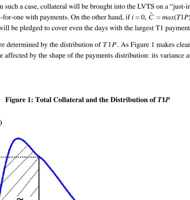
This model is very simple and is designed to be used for illustrative purposes, rather than as a true representation of actual collateral management by LVTS participants. We assume that payments,
, have density function . Figure 1 illustrates a hypothetical FI’s probability
distribution of payments. It reflects the highly skewed nature of FIs’ T1 payments distributions.
Each FI chooses an optimal “normal” level of collateral, , to hold for LVTS purposes, and pledges this collateral to the Bank of Canada before the LVTS opens for processing payments. Normal collateral is locked in for the day and it stays constant from one day to another. One dollar of collateral has an opportunity cost of i per day. Daily T1P becomes known at the beginning of the processing cycle for LVTS payments. If is insufficient to meet payments for the day, the FI must convert higher-yielding securities to those eligible as collateral and bring additional collateral into the LVTS to meet , when payments processing begins. We assume that it is always possible for the FI to obtain sufficient collateral to meet its payment needs. It returns the level of collateral to its normal level at the end of the day. The transactions costs of acquiring securities eligible as collateral and pledging them to the LVTS (and subsequently releasing the pledge) is given by a, which is assumed to be independent of the value of the collateral increase. The additional interest forgone when more collateral must be brought into the LVTS is i times the value of the additional collateral.
The expected total cost, , of collateral is thus given by:
6. See Patinkin (1965), Miller and Orr (1966), Tsiang (1969), and Frenkel and Jovanovic (1980) for analyses of related problems in the context of the demand for money.
T 1P p T 1P( )
C˜
C˜
T 1P
, (1)
where is the proportion of days per year (or the probability each day) that > .
When this occurs, additional collateral of must be brought into the LVTS and a transactions fee must be paid.
The marginal cost equals:
. (2)
Setting the marginal cost to zero (and reordering) defines the optimal level of normal collateral, :
, (3)
, (4)
. (5)
Equation (5) shows that there are both benefits and costs to holding an additional dollar of normal collateral. The benefit is that the chance of having to incur a transactions cost of a is reduced by
. The cost is that, on some occasions when payments are less than normal collateral (this corresponds to ), this extra unit of collateral is unnecessary and will incur an opportunity cost of i.
Rewriting (5),
, (6)
with . (7)
If the opportunity cost is greater than the fixed cost, , then , since the cost of holding any normal collateral exceeds the expected transactions costs of having to move collateral in and
TC i C⋅ ˜ a p T 1P( )dT 1P C˜ ∞
∫
⋅ i (T 1P–C˜)p T 1P( )dT 1P C˜ ∞∫
⋅ + + = p T 1P( )dT 1P C˜ ∞∫
T 1P C˜ T 1P–C˜ MC dTC dC˜ --- i–a p C⋅ ( )˜ i p T 1P( )dT 1P C˜ ∞∫
– = = C˜ i 1 p T 1P( )dT 1P C˜ ∞∫
– ⋅ = a p C⋅ ( )˜ i p T 1P( )dT 1P 0 C˜∫
⋅ = a p C⋅ ( )˜ i G C⋅ ( )˜ = a p C⋅ ( )˜ p C( )˜ G C( )˜ i a --- p C( )˜ G C( )˜ --- Φ( )C˜ = = C˜ Φ–1 i a --- Ω i a --- = = Ω′<0 i>a C˜ = 0out of the LVTS. In such a case, collateral will be brought into the LVTS on a “just-in-time” basis and will move one-for-one with payments. On the other hand, if i = 0, = max(T1P) and enough normal collateral will be pledged to cover even the days with the largest T1 payments.
and are determined by the distribution of . As Figure 1 makes clear, this relationship will be affected by the shape of the payments distribution: its variance and its skewness.
Figure 1: Total Collateral and the Distribution of T1P
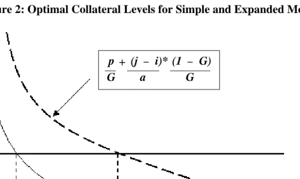
The solid curved line in Figure 2 shows the equilibrium relationship defined by
in equation (6). An increase in i, or a decrease in a, requires an increase in to restore
equilibrium. This requires a reduction in . When the distribution of payments has the skewed shape typical of daily payments sent by LVTS participants, the shape of will be much like that shown in Figure 2, although the degree of curvature of will depend somewhat on the specific parameters of each LVTS participant’s payments distribution.
C˜ p C( )˜ G C( )˜ T 1P P(C)
~
p(T1P) G(C)~
C~
1 – G(C)~
T1P Φ p C( )˜ G C( )˜ ---= Φ C˜ Φ ΦAn increase in the mean of the payments distribution (given that its shape remains constant) increases the normal level of collateral. An increase in the variance of payments increases , because it increases the chance for large payments and reduces the chance that the previous level of collateral will be sufficient to meet payments. Similarly, an increase in the skewness of the payments distribution will increase .
It could be difficult to identify the normal level of collateral in the data. Thus, we would like to know the relationship between average collateral, , and average payments, . Average payments are given by:
. (8)
Average collateral will equal:
. (9)
Thus, average collateral equals normal collateral plus the extra collateral that must be brought into the LVTS whenever payments exceed normal collateral. Average collateral will also vary with average payments. As before, an increase in the variance and skewness of payments will increase average collateral.
Excess collateral is equal to whenever and equals zero when additional collateral must be brought into the LVTS.7 The expected level of excess collateral is thus given by:
(10)
=
.
7. We assume that the extra collateral pledged to the LVTS is exactly what is required to fund T1P.
C˜ C˜ C T 1P T 1P T 1P p T 1P⋅ ( )d(T 1P) 0 ∞
∫
= C C˜ (T 1P–C˜)⋅p T 1P( )d(T 1P) C˜ ∞∫
+ = C˜ –T 1P C˜ >T 1P XC (C˜ –T 1P)⋅ p T 1P( ) 0 C˜∫
dT 1P = C˜ –T 1P ( )⋅ p T 1P( ) 0 ∞∫
dT 1P (T 1P˜ –C˜)⋅ p T 1P( ) C˜ ∞∫
dT 1P + XC = C–T 1PFigure 2: Optimal Collateral Levels for Simple and Expanded Models
4.2
An extended model
The model presented in section 4.1 illustrates in a simple way the problem faced by each FI in deciding how much collateral to pledge to support its LVTS payments; it is not meant to portray the actual decision faced by LVTS participants. The model assumes that the opportunity cost of acquiring collateral at short notice does not differ from i, the ongoing cost of holding a dollar of normal collateral for LVTS purposes. This assumption is not realistic. The equilibrium condition for a model that incorporates this additional factor is given by:
, (11)
where j can be thought of as the opportunity cost of collateral that must be obtained once payments are known at the beginning of the day, if payments exceed normal collateral. The additional third term on the right-hand side of (11) represents the savings associated with holding an additional unit of normal collateral. This savings occurs because, on large payment days, that additional unit does not have to be acquired at a premium price.
(C)
~
simple model C*~
expanded model C~
* simple model p G i a 1 p G (j – i)* a + (1 – G) G C~
MC i G C⋅ ( )˜ –a p C⋅ ( )˜ (j–i) p T 1P( )dT 1P C˜ ∞∫
– 0 = =The first-order condition becomes:
. (12)
The dotted line in Figure 2 graphs this relationship.
In section 6, we test this model to see how well it can explain average holdings of total collateral,
TC1, by FIs in the LVTS. First, however, we consider what measures are appropriate for defining
the variables used in our model.
5.
Empirical Measures of the Variables that Affect the Demand for
Collateral
In assessing the costs of pledging collateral, one must consider what alternatives are available to fund T1 payments. If using collateral is not the least-expensive method, other methods would be chosen.
A participant could wait to receive T1 funds before making outgoing T1 payments. This would not, however, be acceptable for time-sensitive payments. There may be considerable uncertainty about the value and timing of incoming T1 funds. Moreover, delaying payments imposes a cost on other FIs, because their T1 receipts would be delayed. This might delay their own payment outflows, thus leading to a more generalized slowdown or gridlock in the payments system. Hence, to deter this behaviour, LVTS rules require that participants send certain proportions of daily payments by various times during the day.8
A participant could borrow, buy, or swap T1 funds (for T2 funds) from another FI and use the proceeds to fund T1 payments. This would not require any increase in TC1. There is little indication, however, that any significant intraday market for T1 funds currently exists.
To increase its collateral, an FI could pledge additional securities to the LVTS that it already owns, or it could buy or borrow securities on the market that it could use to increase TC1.
5.1
The opportunity cost of holding collateral
We define this to equal the spread between the rate of return on assets pledged as collateral and the rate of return on assets that would be held in the absence of collateral requirements in the LVTS. As a result, the opportunity cost of collateral could differ across financial institutions. According to this definition, if for whatever reason an FI chooses to hold the securities pledged to
8. This rule, however, applies to total LVTS payments sent, not to T1 payments.
i a --- p C( )˜ G C( )˜ --- (j–i) a --- 1–G C( )˜ G C( )˜ --- + Ψ(i j p G, , , ) = =
the LVTS on its books even if the LVTS has no collateral requirements, this collateral has an opportunity cost of zero.
Another definition sometimes used is that the cost of collateral equals the difference between the rate of return on securities pledged as collateral and a bank’s funding costs. This assumes that a bank expands its balance sheet to acquire assets used as collateral. If one uses banker’s
acceptances (BAs) as a measure of a bank’s funding costs and the rate of return on treasury bills as the rate of return on assets pledged as collateral, estimates made a number of years ago put the cost of collateral at 10 to 15 basis points. Recent estimates suggest that this cost has recently fallen, perhaps to as low as 5 basis points.
In November 2001, the list of securities eligible as collateral for the LVTS was expanded at the request of FIs. Eligible collateral now includes corporate debt and many other securities in addition to traditionally used sources of collateral, such as Government of Canada debt. If FIs pledge securities to the LVTS from the expanded list that they were already willing to hold on their balance sheets, the opportunity cost of this new collateral is zero. On the other hand, if they choose to expand their balance sheets to acquire newly eligible securities, most acquired
securities from the expanded list will attract a capital charge. This collateral will therefore have a small opportunity cost. Thus, an estimate of 5 basis points appears to be a reasonable current estimate of the cost of collateral, although it may fluctuate among different FIs.
If an FI needs to buy or borrow large values of securities on the market at very short notice, a premium opportunity cost is probably involved. Some anecdotal evidence puts this cost at more than 40 basis points. Estimates of 5 basis points for normal collateral, and 43 basis points for collateral that is obtained at short notice, will be used as a benchmark in applying our model.
5.2
Monitoring and transactions costs
More active collateral management involves more frequent moves of collateral into and out of the LVTS, so that collateral can be put to higher-yielding uses. It also involves greater transactions costs and requires greater monitoring effort.
Monitoring costs include the value of time and the expertise required to ensure that sufficient collateral is available to support T1 payments. This involves forecasting intraday and day-to-day T1 positions so that it is known ahead of time when additional collateral will be required. It also involves real-time monitoring of an FI’s collateral buffer to ensure that errors in forecasting payments do not prevent payments from flowing as required. The greater the buffer of collateral that is normally pledged to the LVTS, the less effort is necessary for developing accurate
forecasts, and the less actively collateral and net T1 positions must be monitored. Most of these costs may be fixed costs, but there may also be an element of variable cost related to monitoring effort. Unfortunately, no data on monitoring costs are available; therefore, we cannot incorporate this effect into our model.
Transactions costs include the cost of moving collateral into and out of the LVTS. We define them here to also include the transaction cost (but not the interest cost) of buying or borrowing
securities on the market and pledging them to the LVTS. For most LVTS participants, pledging securities to the LVTS that are already owned can be done quickly. In addition to the transactions costs associated with buying or borrowing securities, there would also be a component of
transactions costs that are internal to the FI. The relevant transaction cost would be the sum of these factors. In our base case, we use anecdotal information to estimate a fee of $80 for a “round-trip” transaction; that is, for obtaining and pledging securities to the LVTS and subsequently releasing the pledge.
5.3
The distribution of T1 payment flows
Although our model explains quite clearly the relationship between the distribution of payments and optimal levels of collateral, several additional points should be made.
Our theoretical model focuses on T1P as the determinant of collateral demand in the LVTS. But, as noted in section 2, it is in fact the peak intraday net payments sent that generate daily collateral requirements. On an intraday basis, FIs that receive T1 funds before they need to make T1 payments may need little collateral. Receipts, however, tend to be less predictable than payments sent, especially T1 receipts from other FIs based on client activity. Many T1 payments, a large proportion of which flow to the Bank of Canada, must be made at fixed points during the day. Daily T1P represents the maximum possible daily collateral requirement. The question as to whether FIs focus more on T1 payments or projected peak net T1 payments in determining their daily collateral holdings can be answered by examining how well our model, based on T1P (rather than net payments), performs. In any case, in the absence of data on intraday net T1 positions, we rely on daily T1P.
Many T1 payments sent to and from the Bank are time-sensitive. The Bank of Canada is the banker for the Government of Canada, for the securities settlement system called CDSX, and for the CLS Bank. It is also the settlement agent for the ACSS and the LVTS.9 Most payments and
9. The Automated Clearing Settlement System (ACSS) is used mostly for retail payments. For
descriptions of all these systems, see the Bank of Canada’s Web site at http://www.bankofcanada.ca/ en/payments/mainpage.html.
receipts associated with these functions (as well as others) are due at specific times during the day and are made with T1 funds. Participants cannot delay making payments to the Bank even if T1 funds are expected to be received from the Bank later in the day.
The model that we outlined in section 4 assumes that FIs do not know the value of payments that they will send each day until after they have pledged some collateral, but they know the
distribution that each day’s payments is drawn from. While cash managers at FIs forecast
aggregate payment flows, there will always be residual uncertainty regarding the size of daily T1 payments activity.
Our model also assumes that knowledge of yesterday’s payment values does not help forecast today’s payments—more broadly, that daily payments are identically and independently distributed.10 This is not likely to be strictly accurate. However, there is little first-order
autocorrelation in FIs’ payments distributions, so this seems to be a reasonable approximation.
6.
Applying the Model to the LVTS
The model that we developed in section 4 explains the demand for collateral (TC1) for each FI on the basis of three factors: opportunity costs, transactions costs, and the distribution of T1 payment flows. In this section, we apply the model to each FI to calculate its optimal level of TC1. Then, we sum across all FIs to determine the predicted level of aggregate collateral pledged to the LVTS, and determine how close this is to actual average collateral.11
Predictions from the model are first calculated under the assumption that no premium is
associated with collateral that is obtained at short notice. It is clear, however, that the model will greatly underpredict actual levels of collateral.
Next, we consider our base case, where i = 5 basis points and j = 43 basis points.12 For the transactions costs associated with acquiring and pledging collateral (and later releasing the pledge), we use $80, the estimate outlined earlier. This is the relevant relationship for our
extended model that assumes a premium cost is associated with collateral that is obtained at short notice. We find that actual collateral is quite a bit greater than predicted collateral. As noted above, however, FIs may face different costs of collateral. If we exclude one FI that appears to face a lower cost of collateral, predicted collateral is within 5 per cent of actual.
10. This means that an FI faces exactly the same payments distribution each day. 11. Data on FIs’ payments and collateral are confidential.
To gauge the sensitivity of the results to the values taken by opportunity and transactions costs, several alternative values for these parameters are chosen. First, we consider the effect of halving the transactions cost, from $80 to $40. This generates two opposing effects, as shown in Figure 2: it shifts up the horizontal line given by , which tends to reduce the demand for collateral, but it also shifts up the dashed curve, which tends to increase the demand for collateral. With our data set, the two effects are almost offsetting and there is only a small decrease in the optimal level of collateral.
We then consider the effect of increasing both the normal cost of collateral, i, and the premium cost of collateral, j, by 5 basis points. This shifts up the line in Figure 2, which tends to reduce the demand for collateral and has no effect on the dotted curve. In our data set, the effect on aggregate collateral is large: the average level of collateral would be expected to fall by almost 20 per cent.
Leaving the cost of normal collateral at 10 basis points, we consider the effect of reducing the premium cost of collateral by 5 basis points to 43 basis points. This leaves the line in Figure 2 unchanged and shifts down the dotted line, which tends to reduce the demand for collateral. In aggregate, however, the effect is small, because the demand for collateral falls by only about 3 per cent.
To summarize, our benchmark parameters (i = 5 basis points; j = 43 basis points; a = $80) suggest that, when we take into account one FI that appears to face a lower cost of collateral, the aggregate level of collateral predicted by our model is close to the actual level of collateral. This indicates that, in aggregate and on balance, there is little evidence of “excess” (from an economic
perspective) collateral in the LVTS.
We also calculate optimal coverage ratios associated with our predictions of collateral. For an individual FI, the coverage ratio indicates the per cent of days (or probability each day) that the optimal level of normal collateral, , is sufficient to cover T1P. The aggregate coverage ratio is calculated by averaging the coverage ratios of individual FIs. The aggregate ratio is just over 90 per cent in the base case, indicating that (according to our model), about 10 per cent of the time, FIs would need to bring additional collateral into the LVTS. Thus, if collateral is difficult to obtain at very short notice and if FIs are surprised on those days by having to make large payments, one might expect to see a certain amount of operational disruption and delay in making some payments in the LVTS. Those occasions should, however, be quite rare.
i a ---i a ---i a ---C˜
7.
Analysis Using Panel-Data Regressions of Daily TC1
The previous analysis used a static approach to determine the optimal level of collateral held by FIs. That approach is unable to explain how the demand for collateral has evolved over time in response to changes in the opportunity cost of collateral and FIs’ payment distributions. In this section, we examine this issue using fixed-effects panel-data regressions for the 13 LVTS participants over the period 4 February 1999 to 31 May 2003.13
In line with our theoretical model, we regress TC1 on T1P, the variance of T1P, the skewness of
T1P, and the opportunity cost of collateral.14Since we have no data that capture how the premium cost of collateral and transactions costs vary over time, these variables cannot be included in our regressions. We use a moving 30-day backward window of the variance and skewness of T1P. Our opportunity cost of collateral is based on the spread between 30- or 90-day BAs and treasury bills. After November 2001, when the list of eligible securities for use as collateral in the LVTS was expanded, we take the opportunity cost of collateral to be 5 basis points, in line with the
discussion in section 5. The fixed effects that capture institution-specific unobservable variables are incorporated by including dummy variables in the equations for each FI.
We expect TC1 to respond positively to increases in T1P, and to the variance and skewness of T1P. To the extent that the coverage ratio is high, however, we would expect to see a very small coefficient on T1P (see section 6). A high coverage ratio indicates that, on most occasions, FIs have sufficient collateral to meet daily payment flows and do not have to alter TC1. We would expect TC1 to respond negatively to the opportunity cost.
The panel-data regressions are estimated using the following equations:
Ln(TC1it) = b0i*Di+ b1*Ln(T1Pit) + b2*Ln(varT1Pit) + b3*(skT1Pit) + b4*(OppCost30t) + eit, (13)
Ln(TC1it) = b0i*Di+ b1*Ln(T1Pit) + b2*Ln(varT1Pit) + b3*(skT1Pit) + b4*(OppCost90t) + eit, (14)
where Di represents the institution-specific dummy variables.
The Im, Pesaran, and Shin (2002) tests indicate no evidence of unit roots in our residuals. Breutsch-Pagan tests indicate heteroscedasticity, however, and standard errors are therefore
13. We exclude that part of the sample associated with Y2K effects beginning 1 October 1999 and ending 28 February 2000.
corrected for this effect. The residuals are found to be non-normal. To determine appropriate significance levels, therefore, the distributions of the t-statistics are bootstrapped.
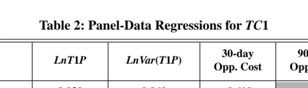
The p-levels are shown in brackets under each estimated coefficient in Table 2. The table shows small but statistically significant coefficients on T1P distribution regressors (T1P, and the variance of T1P). The skewness measure is not statistically significant and is dropped from the regressions. The coefficients on the two yield-spread measures are negative, as expected. The coefficient on the 90-day spread is almost twice the size of that on the 30-day spread. The coefficient estimates found on both 30- and 90-day opportunity costs result in a fairly large dollar-value change in aggregate TC1. For instance, if TC1 is $10 billion, an increase of 5 basis points in the opportunity cost, as measured by the 30-day spread, would reduce TC1 by about $300 million. If we apply the same calculation using the 90-day opportunity cost, TC1 would fall by about $550 million. TC1 therefore appears to be sensitive to the cost of collateral.
The small but significant parameter estimates on T1P and its variance are consistent with the theoretical model, which suggests that FIs would be expected to hold sufficient collateral on a routine basis to cover their payments about 90 per cent of the time. FIs allow for only a small probability of having to increase their total collateral.
Overall, these panel-data regression results are roughly consistent with the predictions made by our theoretical model.
Table 2: Panel-Data Regressions for TC1
LnT1P LnVar(T1P) 30-day Opp. Cost 90-day Opp. Cost TC1 0.030 (0.002) 0.060 (0.004) -0.610 (0.040) TC1 0.030 (0.002) 0.060 (0.004) -1.120 (0.072)
8.
Conclusions
The simple theoretical model that we have developed in this paper appears to explain quite well the amount of collateral pledged to the LVTS, despite the fact that opportunity costs and
transactions costs faced by individual LVTS participants may differ from the benchmark values that we use for those parameters. When we exclude one LVTS participant that appears to face a lower cost of collateral, our model indicates that the actual level of collateral held by FIs is within 5 per cent of the actual level.
Thus, our model suggests that there is little evidence that clients of FIs would be deterred from using the LVTS because FIs passed on to them costs associated with excessive levels of collateral. Our model indicates that the aggregate coverage ratio is about 90 per cent, so that, in aggregate, about 10 per cent of the time, FIs would need to increase TC1 to meet days with very large T1 payments. One might therefore expect to see some occasions when time-sensitive or systemically important payments are delayed as FIs try, on very short notice, to meet unexpectedly large payments; however, those occasions should be rare.
In the empirical part of our paper, we use panel-data regressions to model the demand for collateral as a function of its opportunity cost and measures of an institution’s payments distribution, such as level, variance, and skewness. We find that these regressions are broadly supportive of our theoretical model with small but statistically significant effects for the level and variance (but not the skewness) of an FI’s T1 payments, and with statistically significant and negative effects for the opportunity cost of collateral.
This study suggests several areas for future work. First, in relation to the application of our theoretical model, the use of extreme value theory might strengthen our results. Although we have more than 1,100 observations per FI in our sample, relatively few of these lie in the tail of the payments distribution. Second, more information and a greater understanding of the opportunity costs associated with collateral that is obtained at very short notice would be helpful, because the difference between this cost and the cost of normal collateral is important in explaining the predictions of our model. Finally, our model assumes that FIs can always obtain collateral at short notice, so that stockouts do not occur and payments are not delayed. In practice, if it takes time to obtain collateral needed to make unexpectedly large payments during the day, participants could face financial penalties or reputational damage from delayed payments. These factors would tend to increase the demand for collateral beyond what is predicted by our model. Incorporating these factors would provide a richer model.
Bibliography
Baltagi, B.H. 1995. Econometric Analysis of Panel Data. West Sussex, England: John Wiley & Sons Ltd.
Baumol, W.J. 1952. “The Transactions Demand for Cash: An Inventory Theoretic Approach.”
Quarterly Journal of Economics 66(4): 545–56.
Freedman, C. 1999. The Regulation of Central Securities Depositories and the Linkages between
CSDs and Large-Value Payment Systems. Technical Report No. 87. Ottawa: Bank of
Can-ada.
Frenkel, J.A. and B. Jovanovic. 1980. “On Transactions and Precautionary Demand for Money.”
Quarterly Journal of Economics 95(1): 25–43.
Im, K.S., M.H. Pesaran, and Y. Shin. 2002. “Testing for Unit Roots in Heterogeneous Panels.” Department of Economics, University of Edinburgh.
MacKinnon, J.G. 2002. “Bootstrap Inference in Econometrics.” Canadian Journal of Economics 35(4): 615–45.
Miller, P. and C.A. Northcott. 2002. “CLS Bank: Managing Foreign Exchange Settlement Risk.”
Bank of Canada Review (Autumn): 13–25.
Miller, M.H. and D. Orr. 1966. “A Model of the Demand for Money by Firms.” Quarterly Journal
of Economics 80(3): 413–35.
Patinkin, D. 1965. Money, Interest and Prices. 2nd edition. New York: Harper & Row.
Phillips, P.C.B. 1987. “Time Series Regression with a Unit Root.” Econometrica 55(2): 277–301. Phillips, P.C.B. and P. Perron. 1988. “Testing for a Unit Root in Time Series Regression.”
Biomet-rica 75(2): 335–46.
Schwert, G.W. 1989. “Tests for Unit Roots: A Monte Carlo Investigation.” Journal of Business
and Economic Statistics 7: 147–59.
Tobin, J. 1956. “The Interest-elasticity of Transactions Demand for Cash.” The Review of
Eco-nomics and Statistics 38(3): 241–47.
Tsiang, S.C. 1969. “The Precautionary Demand for Money: An Inventory Theoretical Analysis.”
Working papers are generally published in the language of the author, with an abstract in both official languages. Les documents de travail sont publiés généralement dans la langue utilisée par les auteurs; ils sont
cependant précédés d’un résumé bilingue.
Copies and a complete list of working papers are available from:
Pour obtenir des exemplaires et une liste complète des documents de travail, prière de s’adresser à :
Publications Distribution, Bank of Canada Diffusion des publications, Banque du Canada 234 Wellington Street, Ottawa, Ontario K1A 0G9 234, rue Wellington, Ottawa (Ontario) K1A 0G9 E-mail: [email protected] Adresse électronique : [email protected] Web site: http://www.bankofcanada.ca Site Web : http://www.banqueducanada.ca
2003
2003-35 Real Exchange Rate Persistence in Dynamic General-Equilibrium Sticky-Price Models: An
Analytical Characterization H. Bouakez 2003-34 Governance and Financial Fragility: Evidence from
a Cross-Section of Countries M. Francis 2003-33 Do Peer Group Members Outperform Individual
Borrowers? A Test of Peer Group Lending Using
Canadian Micro-Credit Data R. Gomez and E. Santor 2003-32 The Canadian Phillips Curve and Regime Shifting F. Demers 2003-31 A Simple Test of Simple Rules: Can They Improve How
Monetary Policy is Implemented with Inflation Targets? N. Rowe and D. Tulk 2003-30 Are Wealth Effects Important for Canada? L. Pichette and D. Tremblay 2003-29 Nominal Rigidities and Exchange Rate Pass-Through
in a Structural Model of a Small Open Economy S. Ambler, A. Dib, and N. Rebei 2003-28 An Empirical Analysis of Liquidity and Order
Flow in the Brokered Interdealer Market for
Government of Canada Bonds C. D’Souza, C. Gaa, and J. Yang 2003-27 Monetary Policy in Estimated Models of Small
Open and Closed Economies A. Dib 2003-26 Measuring Interest Rate Expectations in Canada G. Johnson 2003-25 Income Trusts—Understanding the Issues M.R. King 2003-24 Forecasting and Analyzing World Commodity Prices R. Lalonde, Z. Zhu, and F. Demers 2003-23 What Does the Risk-Appetite Index Measure? M. Misina 2003-22 The Construction of Continuity-Adjusted
Monetary Aggregate Components J. Kottaras 2003-21 Dynamic Factor Analysis for Measuring Money P.D. Gilbert and L. Pichette 2003-20 The U.S. Stock Market and Fundamentals: A