Audio-to-Visual Speech Conversion using Deep Neural Networks

Audio-to-Visual Speech Conversion using Deep Neural Networks

[1] University of East Anglia, Norwich, UK

[2] Disney Research, Pittsburgh, USA

[email protected]

,

[email protected]

,

[email protected]

,

[email protected]

We study the problem of mapping from acoustic to visual speech with the goal of generating accurate, perceptually natural speech animation automatically from an audio speech signal. We present a sliding window deep neural network that learns a mapping from a window of acoustic features to a window of visual features from a large audio-visual speech dataset. Overlapping visual predictions are averaged to generate continuous, smoothly varying speech animation. We

outperform a baseline HMM inversion approach in both objective and subjective evaluations and perform a thorough analysis of our results. Index Terms: Audio-to-visual conversion, automatic speech animation, sliding window deep neural networks.

1. Introduction

Audio-to-visual speech conversion is the task of predicting speech-related facial motion from the acoustic signal, or automatically animating the mouth directly from speech. Audio-tovisual speech conversion is useful for applications such as fast content creation for animated productions and low-bandwidth multimodal communication.

Conventional automatic speech animation is performed by first decoding the phonemic content of the speech, and then using the phoneme stream to either interpolate predefined keyshapes [1, 2], stitch together existing speech movements [3–5] or predict visual features using a form of

generative statistical model [6–8]. Although phonemes are speaker independent, they are language dependent and do not encode acoustic cues regarding prosody and emphasis which contribute to the facial pose. This work therefore considers mapping directly from the acoustic signal to animation trajectories which can be used to drive graphics face models.

A variety of approaches have been used to estimate facial motion or visual features automatically from acoustic speech, including multi-linear regression [9], audio-visual codebook learning [10, 11] and a Kalman filter approach [12]. Many approaches rely on non-linear statistical models which are trained on corpora of audio-visual speech and learn a mapping from some acoustic parameterization to a corresponding visual parameterization. A popular approach is to use hidden Markov models (HMMs) [13–18], which have been widely used by the speech community for decades for both speech recognition and synthesis. Chen [14] trained HMMs on joint audio-visual features then separated the models for prediction. For new speech, the visual HMM was sampled using the acoustic state sequence as derived from the Viterbi algorithm. Choi et al. [15] and Terrissi and Gomez [16] also trained joint audio-visual HMMs but ´ used HMM inversion (HMMI) to infer the visual parameters. Xie et al. [17] introduced coupled HMMs (CHMMs) to account for the asynchrony between audio and visual activity caused by coarticulation [19]. Xie et al.’s model incorporated two hidden Markov chains, respectively describing the acoustic and visual information which were

coupled through cross-chain and cross-time conditional probabilities. Both HMMI and CHMM approaches use a maximum likelihood optimization to predict visual features given new audio and the trained model. More recently, Zhang et al. [18] proposed a deep neural network (DNN) to map acoustic features to state posterior probabilities of an audio-visual HMM. Posteriors were converted to HMM emission likelihoods and animation was generated by sampling of the inferred state

sequence. Since the DNN made one prediction per video frame, frequent state switching caused jittery animation. To address this, an optimization function searched for the best state sequence using both the DNN prediction and a cost penalizing state transitions.

An attractive feature of DNNs is that they impose no Gaussian constraints upon the distribution of the data. Hong et al. [20] clustered acoustic features into classes and trained a separate neural network for each class. At the prediction stage, audio features were first classified into one of the classes, and the corresponding neural network was used to estimate the facial pose. A median filter smoothed the inherently discontinuous prediction. To better account for acoustic coarticulatory effects, time-delayed neural networks (TDNNs) and recurrent neural networks (RNNs) have been used. Massaro et al. [21] and Takacs [22] trained TDNNs to map from audio features directly to controls of talking heads using 11 frame input windows. Savran et al. [11] compared RNNs and TDNNs, concluding that a TDNN with 9 frames of audio input centered at the predicted frame performed best. They suggested that this is due to the TDNN’s exposure to acoustic features from both the future and the past, whereas the RNN can only see the past.

Our proposed approach considers carry-over and anticipatory coarticulation in both the acoustic and visual modalities by learning a sliding-window predictor with both windowed input and output. This approach has previously worked well for other spatio-temporal sequence prediction tasks [8] and alleviates the need for arbitrary smoothing, which is necessary for those methods that predict a single frame at a time [20, 21]. Specifically, our contributions can be summarized as follows:

 We extend conventional DNNs with windowed input and output to account for both acoustic and visual coarticulation effects.

 We investigate the level of acoustic detail and audio/visual window size on audio-to-visual conversion accuracy.

 We show that our method outperforms a baseline HMM inversion approach both objectively and subjectively.

 We explore the effectiveness of acoustic speech for predicting visual speech. We discover that sibilant fricative and affricate consonants can be predicted most accurately and velar consonants have highest error.

2. Sliding-Window Deep Neural Network

The goal of this work is to learn a model h(x) := y that can predict a realistic facial pose for any audio speech given audio features x that encode the acoustic speech signal and visual features y that encode the configuration of the lower face. Our approach is inspired by Kim et al.’s [8] sliding window decision tree regression used for automated camera control, sports player tracking and phoneme-driven speech animation. Encouraged by the success of DNNs in the image domain, we instead train a sliding window DNN (SW-DNN) rather than a decision tree. This section describes the SW-DNN framework while implementation details are discussed in Section 3. The following work uses the Theano [23] deep learning library.

We first decompose both audio input X = [x1, x2, . . . xn] and corresponding visual output Y = [y1, y2, . . . yn] into overlapping sequences of fixed-length pairs:

where

wa and wv are the number of features included in the audio and visual window respectively, and n is the total number of features (video frames at 30Hz) in the training set. The size of Y0 is (m ∗ wv) × n, where m is the dimensionality of Y. The overlap is the duration of one video frame and audio

features are extracted such that the window is centered at the video frame. Frames 1 to n index only the video frames that contain speech, so for xj or yj where j < 1 or j > n, the neighbouring silence is included in the encoding. Each column of X0 and Y0 contains a stacked window of audio and visual features and represents one training sample. Model training is performed using backpropagation with Nesterov accelerated momentum gradient descent [24] and a mean squared error (MSE) loss function:

2.2. Audio-to-Visual Conversion

The trained SW-DNN can be used to convert audio speech into a continuous sequence of visual features describing lip motion that is both synchronous with the audio and perceptually accurate. For unseen speech, the first step is to parameterize the audio signal and decompose the features into overlapping sequences of window length wa as per training (Equation 1 (left)). Given the audio features, the SW-DNN predicts a vector which encodes a stacked window of visual features at each time t, ˆy 0 t . The predicted vector is reshaped, giving Yˆ ∗ t , an m ×wv matrix containing the

predicted subsequence at time t. Smooth animation trajectories are generated by overlapping and averaging the subsequences:

where ˆy ∗ t,j is the jth column from the prediction at time t. 3. Experimental Results

Publicly available audio-visual speech datasets are either of limited vocabulary or size [25–27] and provide insufficient data for training a DNN. Instead we use the KB-2k dataset from [4] which is set for future release. KB-2k is a large audio-visual speech dataset containing a male actor speaking ≈2500 phonetically balanced TIMIT sentences in a neutral style. The video is sampled at 30fps and the audio at 48kHz. The dataset has been phonetically transcribed although in this work the phoneme labels are needed only for analysis. 200 sentences were randomly selected to form the test set and validation set (100 of each), and the remaining sentences form the training set. 3.1. Visual Parameterization

A set of 34 2D vertices defines a mesh demarcating the contours of the lips, jaw and the nostrils. An active appearance model (AAM) [28, 29] is used to track and parameterize this facial region in each frame of the video, generating a compact 47 dimensional vector y which encodes both the position and appearance of the area within the mesh for every frame at 30fps. Please refer to [4] for further details of the visual parameterization. This feature set is fixed for all experiments in this paper. 3.2. Audio Parameterization

MFCCs have been the dominant features used for speech recognition for some time. Our MFCC extraction follows broadly the method proposed in the Aurora Distributed Speech Recognition standard [30] and begins by computing the power spectrum of 20ms Hamming windowed frames of audio which are extracted every 10ms. These are input into a 40 channel mel filterbank and a log and discrete cosine transform is applied to give x.

3.3. SW-DNN Training

The model hyper-parameters were selected by performing a randomized grid search [31] over combinations of network size (1-7 hidden layers), layer size (100-4000 units), hidden layer dropout (0-0.9%) and learning rate (0.00001-0.01) using a 260ms window of 40 dimensional MFCCs as input (wa = 24) and a 100ms window of 47 AAM parameters as output (wv = 3). The model with lowest MSE (Equation 3) after 20 epochs on the validation set was trained for a further 180 epochs. The fi- nal model has 3 hidden layers of 2000 rectified linear units [32] with 0.5% dropout and is optimized at a learning rate of 0.0001. The fully connected output layer contains linear units. Batch

normalization is used to speed up convergence. The model takes ≈30 minutes to train on an Nvidia Tesla GPU,and takes just 0.1ms to make a prediction on a CPU, which is fast enough to produce real-time animation.

We investigate the effect of window length by measuring the prediction accuracy of SW-DNNs trained on audio and visual windows of different durations. The key is that the audio window should be large enough to span relevant contextual information that is necessary to predict the facial pose and the visual window is large enough to capture local coarticulatory effects. Table 1 shows MSE computed over the validation set for various audio (columns) and visual (rows) durations. We observe lowest MSE for an audio window of 340ms and visual of 100ms, which is highlighted in the table. This corresponds to using 32 overlapped audio frames and 3 visual frames. The audio window duration is comparable to [8] (367ms), and is longer than [21] (220ms) and [33] (183ms).

Table 1: MSE for SW-DNNs trained on pairs of audio (input) and visual (output) window sizes computed on the validation set. MSE was not computed where the visual window was longer than the audio window (dashes).

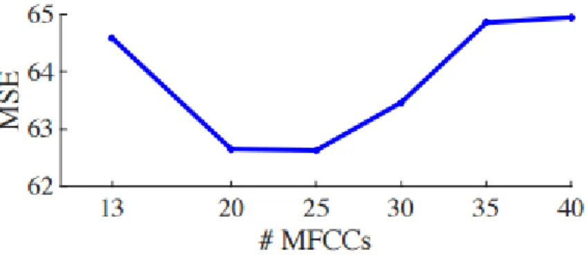
Figure 1: Prediction MSE from DNNs trained using MFCC vectors truncated at various points as acoustic features.

3.5. Quefrency Optimization

MFCCs are typically truncated to give N-dimensional vectors where N = 13 since higher coefficients explain high quefrencies which convey harmonic information [30] . To investigate the optimal number of coefficients for audio-to-visual conversion we train SW-DNNs using N = {13, 20, 25, 30, 35, 40} and measure the MSE of the prediction (Equation 3) on the validation set. The topology of the DNN is fixed (see Section 2) and the audio and visual window sizes are 340 and 100ms

respectively. Figure 1 shows the MSE as a function of the number of MFCCs. The MSE decreases as more coefficients are included up to 25 and then increases as more coefficients are retained. This suggests that coefficients over 13 should be retained in audio-to-visual conversion as these higher quefrencies contribute to prediction accuracy.

We benchmark our method against Choi et al.’s HMM inversion (HMMI) approach since HMMI was shown to outperform a number of HMM-based techniques in an experimental comparison [33]. Our implementation of HMMI followed closely the method described in [15] in which MFCCs were extracted at 10ms non-overlapping frames and the corresponding visual features were upsampled to 100fps using a cubic spline. These features are used to train joint audio-visual phoneme-based HMMs with 3 states and 3 mixtures. Inversion is performed using a recursive Baum-Welch optimization.

Each of the 100 test sentences (8470 samples) were predicted using both HMMI and our proposed sliding window DNN framework (SW-DNN). The SW-DNN trajectories were constructed from the predicted overlapping subsequences (see Equation 4) and error was computed in 47 dimensional visual feature space for both approaches. Table 2 shows the MSE and standard error (SE) over the 100 test sentences measured against ground truth. We observe that SW-DNN generates lower error (59.2) than HMMI (88.9), with a significance level of p 0.001 according to one-way ANOVA analysis. We also report the correlation coefficient (CC) of both methods and observe higher correlation with SW-DNN than HMMI at 0.83 and 0.74 respectively.

Table 2: MSE with standard error (SE), and correlation coeffi- cient (CC) over the test sentences measured against ground truth for SW-DNN prediction and HMMI.

Figure 2: The mean rating for 20 test sentences where 1=real and 0=synthesized. Blue bars show results for ground truth (GT), green for SW-DNN and yellow for HMMI.

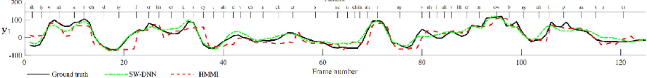
For illustration, Figure 3 shows the first dimension of the predicted visual features with phoneme labels for both SWDNN (blue) and HMMI (red) against the ground truth features which were extracted from the tracked video for the sentence “She was ready for her great adventures and the arrival of her mobile partner”. It can be observed that not only does our approach more closely follow the ground truth trajectory, but that it is smoothly varying and requires no smoothing, whereas the HMMI approach is discontinuous and makes abrupt changes at phoneme boundaries due to frequent state transitions. Rendered examples of test sentences can be found at:

https://www.uea.ac.uk/computing/speech-languageand-audio-processing/automatic-speech-animation.

3.7. Subjective Evaluation

Twenty test sentences were randomly selected and rendered from the encoded visual features under three conditions; ground truth (GT), SW-DNN and HMMI. The ground truth condition was included to measure the error introduced by rendering artefacts from the visual parameterization to attain a performance goal for our approach. Each sentence was presented in a randomized order to participants who were asked whether they deemed the lip motion real or synthesized under a forced choice binary condition. The experiment was performed using a web interface and participants were recruited by sharing the URL on social media. The first five responses from each participant were omitted from analysis to allow subjects to familiarize themselves with the task, leaving an average of 26 responses per sentence. Figure 2 shows the mean rating for each sentence under each condition. We observe that SW-DNN almost always outperforms HMMI in terms of perceived realism. Overall, the HMMI predictions were perceived as real 19% of the time, SWDNN 58% and GT 78%. This means that almost 60% of the time our approach predicts facial motion that is perceived as real. This is appreciable, since humans are adept at recognizing subtle audio-visual discrepancies, so even a single incorrect lip motion will affect the overall perception of realism.

Figure 3: Comparing predictions of our sliding window DNN (SW-DNN) and HMM inversion (HMMI) for the first visual feature which encodes the openness of the mouth.

Figure 4: MSE per phoneme in the testing set. The label /sp/ denotes a mid-sentence short pause. 3.8. Analysis of Prediction

To investigate further the effectiveness of the acoustic signal for predicting visual speech we calculate the MSE for each phoneme in the testing set. These are ranked and plotted in Figure 4. Interestingly, the four consonants with lowest MSE are all sibilant fricatives (/zh, z, sh, s/). These are followed by affricates /jh, ch/, which are characterized by a plosive followed by a sibilant fricative. The remaining non-sibilant fricative consonants (/f, v, hh, dh, th/) are spread across the graph. One explanation for this is that since fricatives are produced by forcing air through a narrow channel, a turbulent airflow focuses energy at higher frequencies. Sibilants are particularly characteristic as they are made by directing a stream of air towards the teeth and are typically louder and contain energy at higher frequencies than non-sibilants, giving rise to distinctive acoustic features. Furthermore, the lip configurations of /zh, ch, sh, jh/ and /s, z/ are known to be somewhat interchangeable since each group has the same place of articulation. This means that the model need not discriminate between phonemes within the respective groups to predict an accurate lip pose.

Towards the right of Figure 4 we observe high MSE for the velar consonants /g, k, ng/. These are articulated with the tongue dorsum against the velum, a mechanism that occurs fully at the rear of the mouth. Since the lips do not contribute to the production of these sounds, they are highly influenced by visual coarticulation.

The MSE peaks at /sp/, which denotes a short pause that occurs mid-way through an utterance. Intuitively, MFCCs encode silence or non-speech related sounds during pauses, such as inhalation, during which the lip pose is difficult to predict. This is especially true for pauses longer than the 340ms audio window since no context is provided to guide the model prediction. This prompted an investigation into the effect of phoneme duration on accuracy.

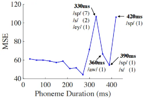
Figure 5 shows MSE plotted against phoneme duration. Over 90% of the phonemes in our data have a duration of 120ms or less and a small number have a duration greater than 330ms, which are listed on the figure. We observe a decrease in MSE as phoneme duration increases up until 300ms which is around the same duration as the acoustic input window of 340ms. This spike contains 7 examples of /sp/, somewhat confirming the dif- ficulty in predicting the lip pose for mid-sentence pauses of a longer length. Across all phonemes we measure a correlation coefficient of just 0.09 between phoneme duration and MSE, so duration does not play a significant role in the overall quality of audio-to-visual conversion.

Figure 5: MSE against phoneme duration in milliseconds. The phonemes with longer durations are listed.

4. Conclusions

In this paper we have introduced a sliding window deep neural network model for audio-to-visual conversion, with windowed acoustic input and visual output. The method requires no phonetic annotation or smoothing of the output. Prediction is fast and results in lower mean squared error, a higher correlation coefficient and more perceptually realistic animation than a baseline HMM inversion technique.

Experimentally we determined that using a 340ms acoustic window to train a three-layer neural network to predict 100ms visual output provided optimal results. We discovered that retaining 25 MFCCs gave best prediction performance. Analysis shows that the lip pose for sibilant fricatives can most accurately be predicted from the acoustic signal and velar consonants and mid-sentence pauses are more difficult.

Along with the pixel intensities, the visual parameterization encodes the shape of the actor’s mouth which can be retargeted to graphics characters using deformation transfer for example. Future work will focus on incorporating the proposed method into a real-time speech driven animation pipeline. 5. References

[1] M. Cohen and D. Massaro, “Modeling coarticulation in synthetic visual speech,” in Models and Techniques in Computer Animation, N. Thalmann and T. D, Eds. Springer-Verlag, 1994, pp. 141–155. [2] T. Ezzat, G. Geiger, and T. Poggio, “Trainable videorealistic speech animation,” in Proceedings of SIGGRAPH, 2002, pp. 388– 398.

[3] C. Bregler, M. Covell, and M. Slaney, “Video rewrite: Driving visual speech with audio,” in Proceedings of SIGGRAPH, 1997, pp. 353–360.

[4] S. L. Taylor, M. Mahler, B.-J. Theobald, and I. Matthews, “Dynamic units of visual speech,” in Proceedings of the 11th ACM SIGGRAPH/Eurographics conference on Computer Animation. Eurographics Association, 2012, pp. 275–284.

[5] W. Mattheyses, L. Latacz, and W. Verhelst, “Automatic viseme clustering for audiovisual speech synthesis,” in Proceedings of Interspeech, 2011.

[6] R. Anderson, B. Stenger, V. Wan, and R. Cipolla, “Expressive visual text-to-speech using active appearance models,” in Proccedings of the International Conference on Computer Vision and Pattern Recognition, 2013, pp. 3382–3389.

[7] B. Fan, L. Wang, F. K. Soong, and L. Xie, “Photo-real talking head with deep bidirectional lstm,” in Proceedings of the International Conference on Acoustics, Speech, and Signal Processing. IEEE, 2015. [8] T. Kim, Y. Yue, S. Taylor, and I. Matthews, “A decision tree framework for spatiotemporal

sequence prediction,” in Proceedings of the 21th ACM SIGKDD International Conference on Knowledge Discovery and Data Mining, ser. KDD ’15, 2015, pp. 577–586.

[9] M. S. Craig, P. van Lieshout, and W. Wong, “A linear model of acoustic-to-facial mapping: Model parameters, data set size, and generalization across speakers,” The Journal of the Acoustical Society of America, vol. 124, no. 5, pp. 3183–3190, 2008.

[10] R. Gutierrez-Osuna, P. K. Kakumanu, A. Esposito, O. N. Garcia, A. Bojorquez, J. L. Castillo, and I. Rudomin, “Speech-driven fa- ´ cial animation with realistic dynamics,” Multimedia, IEEE Transactions on, vol. 7, no. 1, pp. 33–42, 2005.

[11] A. Savran, L. M. Arslan, and L. Akarun, “Speaker-independent 3D face synthesis driven by speech and text,” Signal processing, vol. 86, no. 10, pp. 2932–2951, 2006.

[12] T. Lehn-Schiøler, L. K. Hansen, and J. Larsen, “Mapping from speech to images using continuous state space models,” in Machine Learning for Multimodal Interaction. Springer, 2005, pp. 136–145.

[13] M. Brand, “Voice puppetry,” in Proceedings of the 26th annual conference on Computer graphics and interactive techniques. ACM Press/Addison-Wesley Publishing Co., 1999, pp. 21–28. [14] T. Chen, “Audiovisual speech processing,” Signal Processing Magazine, IEEE, vol. 18, no. 1, pp. 9– 21, 2001.

[15] K. Choi, Y. Luo, and J.-N. Hwang, “Hidden markov model inversion for audio-to-visual conversion in an MPEG-4 facial animation system,” Journal of VLSI signal processing systems for signal, image and video technology, vol. 29, no. 1-2, pp. 51–61, 2001.

[16] L. D. Terissi and J. C. Gomez, “Audio-to-visual conversion via ´ HMM inversion for speech-driven facial animation,” in Advances in Artificial Intelligence-SBIA 2008. Springer, 2008, pp. 33–42. [17] L. Xie and Z.-Q. Liu, “A coupled HMM approach to videorealistic speech animation,” Pattern Recognition, vol. 40, no. 8, pp. 2325–2340, 2007.

[18] X. Zhang, L. Wang, G. Li, F. Seide, and F. K. Soong, “A new language independent, photo-realistic talking head driven by voice only.” in Interspeech, 2013, pp. 2743–2747.

[19] C. Bregler and Y. Konig, ““Eigenlips” for robust speech recognition,” in Acoustics, Speech, and Signal Processing, 1994. ICASSP-94., 1994 IEEE International Conference on, vol. 2. IEEE, 1994, pp. II– 669.

[20] P. Hong, Z. Wen, and T. S. Huang, “Real-time speech-driven face animation with expressions using neural networks,” Neural Networks, IEEE Transactions on, vol. 13, no. 4, pp. 916–927, 2002. [21] D. W. Massaro, J. Beskow, M. M. Cohen, C. L. Fry, and T. Rodgriguez, “Picture my voice: Audio to visual speech synthesis using artificial neural networks,” in AVSP’99-International Conference on Auditory-Visual Speech Processing, 1999.

[22] G. Takacs, “Direct, modular and hybrid audio to visual speech ´ conversion methods-a comparative study.” in Interspeech, 2009, pp. 2267–2270.

[23] J. Bergstra, O. Breuleux, F. Bastien, P. Lamblin, R. Pascanu, G. Desjardins, J. Turian, D. Warde-Farley, and Y. Bengio, “Theano: a CPU and GPU math expression compiler,” in Proceedings of the Python for Scientific Computing Conference (SciPy), Jun. 2010, oral Presentation.

[24] Y. Nesterov, “A method for unconstrained convex minimization problem with the rate of convergence o (1/k2),” in Doklady an SSSR, vol. 269, no. 3, 1983, pp. 543–547.

[25] E. K. Patterson, S. Gurbuz, Z. Tufekci, and J. N. Gowdy, “Cuave: A new audio-visual database for multimodal human-computer interface research,” in Acoustics, Speech, and Signal Processing (ICASSP), 2002 IEEE International Conference on, vol. 2. IEEE, 2002, pp. II–2017.

[26] M. Cooke, J. Barker, S. Cunningham, and X. Shao, “An audiovisual corpus for speech perception and automatic speech recognition,” The Journal of the Acoustical Society of America, vol. 120, no. 5, pp. 2421–2424, 2006.

[27] K. Messer, J. Matas, J. Kittler, J. Luettin, and G. Maitre, “Xm2vtsdb: The extended m2vts database,” in Second international conference on audio and video-based biometric person authentication, vol. 964. Citeseer, 1999, pp. 965–966.

[28] T. Cootes, G. Edwards, and C. Taylor, “Active appearance models,” IEEE Transactions on Pattern Analysis and Machine Intelligence, vol. 23, no. 6, pp. 681–685, 2001.

[29] I. Matthews and S. Baker, “Active appearance models revisited,” International Journal of Computer Vision, vol. 60, no. 2, pp. 135– 164, 2004.

[30] ETSI, “Speech Processing, Transmission and Quality Aspects (STQ); Distributed speech recognition; Extended advanced frontend feature extraction algorithm; Compression algorithms; Backend speech reconstruction algorithm,” ETSI STQ-Aurora DSR Working Group, ES 202 212 version 1.1.1, Nov. 2003.

[31] J. Bergstra and Y. Bengio, “Random search for hyper-parameter optimization,” The Journal of Machine Learning Research, vol. 13, no. 1, pp. 281–305, 2012.

[32] V. Nair and G. E. Hinton, “Rectified linear units improve restricted boltzmann machines,” in Proceedings of the 27th International Conference on Machine Learning (ICML-10), 2010, pp. 807– 814.

[33] S. Fu, R. Gutierrez-Osuna, A. Esposito, P. K. Kakumanu, and O. N. Garcia, “Audio/visual mapping with cross-modal hidden markov models,” Multimedia, IEEE Transactions on, vol. 7, no. 2, pp. 243– 252, 2005.