S. Nickel, F. Saldanha-da-Gama, H.-P. Ziegler
Stochastic programming approaches
for risk aware supply chain network
design problems
© Fraunhofer-Institut für Techno- und Wirtschaftsmathematik ITWM 2010 ISSN 1434-9973
Bericht 181 (2010)
Alle Rechte vorbehalten. Ohne ausdrückliche schriftliche Genehmigung des Herausgebers ist es nicht gestattet, das Buch oder Teile daraus in irgendeiner Form durch Fotokopie, Mikrofilm oder andere Verfahren zu reproduzieren oder in eine für Maschinen, insbesondere Datenverarbei tungsanlagen, ver-wendbare Sprache zu übertragen. Dasselbe gilt für das Recht der öffentlichen Wiedergabe.
Warennamen werden ohne Gewährleistung der freien Verwendbarkeit benutzt. Die Veröffentlichungen in der Berichtsreihe des Fraunhofer ITWM können bezogen werden über:
Fraunhofer-Institut für Techno- und Wirtschaftsmathematik ITWM Fraunhofer-Platz 1 67663 Kaiserslautern Germany Telefon: +49 (0) 6 31/3 16 00-0 Telefax: +49 (0) 6 31/3 16 00-10 99 E-Mail: [email protected]
Vorwort
Das Tätigkeitsfeld des Fraunhofer-Instituts für Techno- und Wirtschaftsmathematik ITWM umfasst anwendungsnahe Grundlagenforschung, angewandte Forschung sowie Beratung und kundenspezifische Lösungen auf allen Gebieten, die für Tech-no- und Wirtschaftsmathematik bedeutsam sind.
In der Reihe »Berichte des Fraunhofer ITWM« soll die Arbeit des Instituts kontinu-ierlich einer interessierten Öffentlichkeit in Industrie, Wirtschaft und Wissenschaft vorgestellt werden. Durch die enge Verzahnung mit dem Fachbereich Mathema-tik der Universität Kaiserslautern sowie durch zahlreiche Kooperationen mit inter-nationalen Institutionen und Hochschulen in den Bereichen Ausbildung und For-schung ist ein großes Potenzial für ForFor-schungsberichte vorhanden. In die Bericht-reihe werden sowohl hervorragende Diplom- und Projektarbeiten und Disserta-tionen als auch Forschungsberichte der Institutsmitarbeiter und Institutsgäste zu aktuellen Fragen der Techno- und Wirtschaftsmathematik aufgenommen. Darüber hinaus bietet die Reihe ein Forum für die Berichterstattung über die zahl-reichen Kooperationsprojekte des Instituts mit Partnern aus Industrie und Wirt-schaft.
Berichterstattung heißt hier Dokumentation des Transfers aktueller Ergebnisse aus mathematischer Forschungs- und Entwicklungsarbeit in industrielle Anwendungen und Softwareprodukte – und umgekehrt, denn Probleme der Praxis generieren neue interessante mathematische Fragestellungen.
Prof. Dr. Dieter Prätzel-Wolters Institutsleiter
Stochastic Programming approaches for Risk aware Supply
Chain Network Design Problems
Stefan Nickela,b, Francisco Saldanha-da-Gamac, Hans-Peter Zieglera∗
a Institute for Operations Research, Karlsruhe Institute of Technology (KIT), Karlsruhe, Germany b Fraunhofer Institute for Industrial Mathematics (ITWM), Kaiserslautern, Germany
c DEIO-CIO, Faculdade de Ciˆencias, Universidade de Lisboa, Lisboa, Portugal
April 12, 2010
Abstract
In this paper, a multi-period supply chain network design problem is addressed. Sev-eral aspects of practical relevance are considered such as those related with the financial decisions that must be accounted for by a company managing a supply chain. The deci-sions to be made comprise the location of the facilities, the flow of commodities and the investments to make in alternative activities to those directly related with the supply chain design. Uncertainty is assumed for demand and interest rates, which is described by a set of scenarios. Therefore, for the entire planning horizon, a tree of scenarios is built. A target is set for the return on investment and the risk of falling below it is measured and accounted for. The service level is also measured and included in the objective function. The problem is formulated as a multi-stage stochastic mixed-integer linear programming problem. The goal is to maximize the total financial benefit. An alternative formulation which is based upon the paths in the scenario tree is also proposed. A methodology for measuring the value of the stochastic solution in this problem is discussed. Computational tests using randomly generated data are presented showing that the stochastic approach is worth considering in these type of problems.
Keywords: Supply Chain Management, Multi-stage Stochastic Programming, Financial Decisions, Risk.
1
Introduction
Structuring a global supply chain is a complex decision making process. The complexity arises from the need to integrate several decisions each of which with a relevant contribution to the performance of the whole system. In such problems, the typical input includes a set of markets, a set of products to be manufactured and/or distributed, demand forecasts for the different markets and some information about future conditions (e.g. production and transportation costs). Making use of the above information, companies must decide where facilities (e.g.
∗
plants, distribution centers) should be set operating, how to allocate procurement/production activities to the different facilities, and how to plan the transportation of products through the supply chain network in order to satisfy customer demands. Often, the objective considered is the minimization of the costs for building and operating the network.
Historically, researchers have focused relatively early on the design of production/distri-bution systems (see Geoffrion and Powers [8]). Typically, discrete facility location models were proposed which possibly included some additional features but that still had a limited scope and were not able to deal with many realistic supply chain requirements. However, in the last decade, much research has been done to progressively develop more comprehensive (but tractable) models that can better capture the essence of many supply chain network design (SCND) problems and become a useful tool in the decision making process. This can be seen in the papers by Melo et al. [24] and Shapiro [32], where it also becomes clear that many aspects of practical relevance in supply chain management (SCM) are still far from being fully integrated in the models existing in the literature.
As pointed out by Shapiro [32], in corporate planning, financial decisions may strongly interact with the supply chain planning. In fact, structuring and managing a supply chain is often just part of a whole set of activities associated with a company. Accordingly, the invest-ments in the supply chain must be integrated with other profitable investinvest-ments. Typically, several points in time can be considered, in which the investments can be made or in which their return can occur (which in turn, may allow further investments in the supply chain). Additionally, due to the large capital often associated with the network design decisions, the possibility of taking advantage of some investment opportunity is often considered, which justifies the use of loans.
The evaluation of the investments made in a supply chain is usually based on their return rate. This fact calls for the inclusion of revenues in SCND models, which also gives the possibility of setting a target for the return on investment (ROI). The inclusion of the ROI in SCND models has not received attention in the literature.
In addition to the financial aspects just mentioned the multi-period nature of some de-cisions has often to be accommodated in SCND models. Usually, a supply chain network has to be in use for some time during which the underlying conditions may change. In some situations, a single-period facility location model may be enough to find a “robust” network design. However, in most cases, it is possible and even desirable to allow a change in the de-cisions in order to better absorb the changes in the parameters and thus to adjust the system accordingly. Location decisions are often among such decisions. In such cases, typically, there is a discrete set of points in time in which changes can be made in the network structure. These points allow a partition of the planning horizon into several time periods and constitute
the initial setting for a multi-period network design problem. As pointed out by Melo et al. [23] the existence of a periodic budget (e.g. annual, quarterly) for investments in the supply chain is also a situation requiring the use of a multi-period modeling framework.
Another feature that can hardly be avoided in many SCND problems regards the uncer-tainty associated to the future conditions which may influence the input of the problem, and the need to include this uncertainty in the models supporting the decision making process. Different sources of uncertainty exist that can be included in the models (see Snyder [33]) such as demand, production or distribution costs, supply of raw materials etc. The uncertainty existing in the data leads to the need to find robust SCND decisions and/or consider ways for measuring and optimizing the risk associated with those decisions.
A constraint often considered in the literature devoted to SCND problems is that all the demand must be supplied throughout the planning horizon. However, for several reasons such constraint may become meaningless. Firstly, because demand is uncertain. Secondly because due to the existence of other investments in alternative to those that can be made in the supply chain, the company may find it better not to invest in a supply chain the amount needed to assure the complete demand satisfaction. Finally, it may simply be a marketing strategy not to supply all the demand in some time horizon. Taking these arguments into consideration, a more interesting and from a practical point of view more reasonable alternative is to measure the service level (e.g. the proportion of satisfied demand) and to reward it in the objective function.
1.1 Problem Description
This paper is the first one which discusses a SCND problem capturing all the above men-tioned aspects. We consider a supply chain network design problem with multiple periods, stochasticity, financial decisions and risk (SCN DM SF R). The planning horizon is divided into several time periods in each of which several decisions can be made namely, i) the facilities that should be operating and thus the investments to make in the supply chain structure, ii) other investments to make in addition to the previous ones, iii) the loans to get and iv) the flow of commodities through the network. Stochasticity is considered for the demand and for the interest rates. A set of scenarios is considered for describing the uncertainty. Revenues are included in the model as well as the ROI. The service level for each customer is evaluated and weighted in the objective function. Finally, a measure of risk is introduced. The objective is to minimize the overall cost which is evaluated considering the investments made, the revenues, and the transportation costs.
deriving the the deterministic equivalent program. A more simplified and from a computa-tional point of view more attractive formulation is presented afterwards, which is a formulation based on the paths in the scenario tree.
1.2 Current State-of-the-Art
Several papers can be found in the literature addressing multi-period, multi-commodity SCND problems. Fleischmann et al. [7] consider a problem in which the decisions to be made regard location, distribution, capacity and production. The objective is to optimize the net present value. In a problem studied by Hugo and Pistikopoulos [18] the decisions involve location, distribution and capacity of the facilities. Two objectives are considered: the net present value (to maximize) and the potential environmental impact (to minimize). Ulstein et al. [35] consider the location of a single echelon of facilities. The decisions also involve the flow of commodities through the network and the capacity of the facilities. A profit maximization objective is considered.
Canel et al. [5] consider a SCND problem and search for the best location for a set of intermediate facilities in a two-layer network as well as for the best way for shipping the commodities through the network. Hinojosa et al. [14], Hinojosa et al. [15] and Vila et al. [36] consider two location layers with location decisions to be made for both layers. In the first paper, location and shipment decisions are considered. The second paper considers addition-ally, inventory and procurement decisions. The third paper considers location, production, shipment, inventory and capacity decisions. Finally, Melo et al. [23] consider a generic num-ber of echelons with the possibility of making location decisions in all layers. Production, distribution, procurement and capacity decisions are also considered.
The inclusion of uncertainty in SCND problems in general and in facility location models in particular is not new and has been addressed by many authors (see Snyder [33]). Neverthe-less, as pointed out by Melo et al. [24], the scope of the models that have been proposed is still rather limited due to the natural complexity of many stochastic optimization problems. In particular, most of the literature considers single-period single-commodity problems. Never-theless, several papers can be found addressing multi-commodity problems in a single-period context. This is the case in the problems studied by Guill´en et al. [11], Liste¸s and Dekker [21], Sabri and Beamon [29] and Santoso et al. [30]. These authors consider two to multiple echelons. The decisions concern the flow of commodities, capacities, production or procure-ment and inventory decisions. Stochasticity is assumed for the demand, the production costs and the delivery costs, respectively and the objectives concern the profit, the net revenue, the costs, the demand satisfaction or just the flexibility (regarding the volume or delivery).
Aghez-zaf [1] although considering only a single commodity. Two facility layers are considered with location decisions being made for just one of them. In addition to the location decisions, distribution, inventory and capacity decisions are also considered. The latter refer to the pos-sibility of expanding the capacity of the facilities. Stochasticity is assumed for the demands. A robust optimization approach is proposed for the problem.
As mentioned above, the possibility of not satisfying all the demand makes sense in many SCND problems. This possibility has been modeled by a few authors. Sabri and Beamon [29] consider the service level as one objective function to maximize in a bi-objective optimization problem. Hwang [19] consider a single-commodity SCND problem with two facility layers. Location as well as routing decisions are considered. Stochasticity is associated with traveling time (assumed to have a known distribution). A minimum service level is imposed which is done in terms of the number of facilities to be establish the goal is to assure a minimum probability for a customer to be covered which is expressed via a function of the distance and the travel time between the facilities and the customers. The objective is to minimize the number of facilities established.
The inclusion of risk management in SCND problems has been addressed in the literature although in rather limited settings. Lowe et al. [22] measure the risk associated with ex-change rates fluctuation. A single-commodity, single-echelon problem is considered. Despite the inclusion of several multi-period factors involved in the problem, the location decisions are static. In addition to these decisions, production, procurement and capacity of the fa-cilities decisions are also part of the decision making process. A two-phase multi-screening approach is proposed taking into account several cost factors. Goh et al. [9] consider a single-commodity, single-period, single-layer facility location problem. Transportation decisions are also considered. Stochasticity is assumed for the demand and for the exchange rates. Several risks are considered namely those related with supply, demand, exchange, and disruption. Two objectives are handled: profit maximization and risk minimization.
The inclusion of uncertainty in supply chain management problems leads often to the need to consider stochastic programming approaches. Not many papers exist with such approaches for SCND problems although a few can be referred. In Sch¨utz et al. [31] and Liste¸s [20] two-stage stochastic programming formulations are considered. Alonso-Ayuso et al. [4] present a two-stage stochastic programming model for multi-period single-commodity supply chain planning problem. Uncertainty is assumed for product net price, demand, raw material supply and production costs. No location decisions are made but it is possible to make decisions regarding the capacity of the facilities which can change throughout the planning horizon. Mitra et al. [25] provide an overview on the literature addressing stochastic supply chain management problems namely those arising in the context of SCND.
The use of a multi-period setting can lead to a multi-stage stochastic programming prob-lem. Several papers can be found in the literature addressing such situation. Tarhan and Grossmann [34] consider a multi-stage stochastic programming approach for a multi-period problem in process networks where the decisions regard the expansion of capacity processes, the operation or not of the processes and the possibility of installing pilot plants for some processes. Nowak and R¨omisch [27] consider a multi-stage stochastic programming model for the weekly generation of electric power under uncertain demand. A multi-period model is considered. Ahmed et al. [3] present a multi-stage stochastic programming model for a multi-period capacity expansion problem. Demands are uncertain as well as the investment costs.
The multi-stage nature of many of the above problems adds complexity to the problems. Several theoretical developments can be found in the literature for these types of problems. Recently, Guan et al. [10] presented a general method for multistage stochastic integer pro-gramming which combines inequalities that are valid for individual scenarios. When a set of scenarios is assumed for modeling uncertainty in a multi-stage setting, it is possible to build a scenario tree. In such a case, as shown in R¨omisch and Schultz [28] an alternative modeling framework can be proposed which is based in the paths in the tree. Huang and Ahmed [17] use such modeling framework as a mean to better model the evolution of the uncertainties in a multi-stage stochastic problem. The authors show that with the use of a multistage formulation more information about the uncertainties is revealed which can be absorbed by the decisions.
Finally, an important issue when a set of scenarios is considered for describing the uncer-tainty, is how to obtain the scenarios. Several methodologies can be used for doing so. The reader can refer to Heitsch and R¨omisch [12], Heitsch and R¨omisch [13], Hoyland and Wallace [16] and M¨oller et al. [26].
The remainder of the paper is organized as follows. In the next section the details about the problem studied in this paper are given. In section 3 the problem is formulated as a multi-stage stochastic programming problem. In section 4 an alternative formulation is proposed which is a path-in-the-scenario-tree-based formulation. Section 5 discusses the value of multi-stage stochastic programming in the context of SCND. In section 6 we present the computational tests performed. The paper ends with some conclusions driven by the work done.
2
Problem description
The basic setting for SCN DM SF R is defined by a supply chain with two echelons: facilities (e.g. warehouses or distribution centers) and customers. A planning horizon divided into several time periods is considered. In each period, customers have to be supplied with multiple commodities from the operating facilities according to their demand and to the operating capacity. It is possible to make direct investments in the supply chain (e.g. set facilities operating) and to make other investments. Uncertainty is associated with demands and return rates. In order to capture potentially interesting investments, loans are also possible. We consider a measure for the service level. A target is set for the ROI and the risk of falling below it is measured and considered in the decision making process. The goal is to find optimal decisions in each period concerning the location of the facilities, the investments to make and the flow of commodities through the network. We detail next all these relevant aspects concerning SCN DM SF R.
2.1 Dealing with uncertainty
As mentioned above, uncertainty is associated with demand and return rates. These quantities can, in principle, be represented by random variables but we assume that all random variables are dependent and completely determined by some state of nature. Accordingly, we assume that a set of events/scenarios can be considered that fully determines the values of all the uncertain parameters.
In practice, we would start by considering the set of events determining the demand and the (possibly different) set of events determining return rates. Nevertheless, by combining both types of events we would be led to a new set of events determining simultaneously demand and return rates. This is the situation we consider directly in this paper. We do so for the sake of simplicity when formulating SCN DM SF R and also because from a computational point of view it is not relevant how the scenarios are built. For further information about scenario generation and reduction in optimization problems under uncertainty the reader can refer to Heitsch and R¨omisch [13] and Hoyland and Wallace [16].
2.2 Decisions
Four types of decisions are considered inSCN DM SF R: i) Where to set facilities operating, ii) which investments to make, iii) which loans to consider, and iv) how to ship the commodities from the operating facilities to the customers. All these decisions have to be made for each period of the planning horizon.
to be made before knowing which event will occur and thus before knowing the demand and the interest rates. In each time period, shipment decisions will be made only after demand is disclosured. Accordingly, such decisions will be a recourse decisions in the sense that the best decisions will be made taking into account the decisions already implemented before knowing the even that occurs. The decisions made in the beginning of each time period, apart from the first one, will have the role of recourse decisions for the decisions made before. This is easily explained due to the impact that the investment decisions will have in the future availability of financial resources.
We allow the location decisions to change from one period to the following i.e., we allow multiple opening and closing of facilities throughout the planning horizon. This makes sense with facilities such as warehouses or distribution centers. We might think that as a conse-quence, the location decisions would only have an effect in the time period in which they are made. However, this is not necessarily true because the fact that some money is devoted to set facilities operating may prevent us from making other investments that might have a return in a distant future.
We assume that the revenue for deliveries occur only in the end of the time period. Thus, we are assuming that the customers only regularize their debts in the end of the time periods. No generality is lost with this assumption because we can report the revenue values to any moment in time. However, this assumption helps making the model we propose more easy-reading.
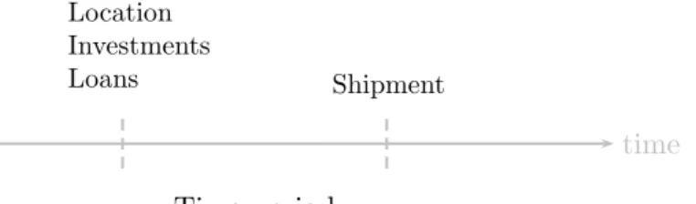
Figure 1 illustrates the decisions to be made in a generic time period.
time
Time period Location
Investments
Loans Shipment
Figure 1: Decisions in each time period.
2.3 Investments
Several types of investments can be considered for a company managing a supply chain namely, direct investments in the supply chain, indirect investments in the supply chain, and alternative investments to these ones.
structure. This may include, for instance, land acquisition for building facilities or renting a facility.
Indirect investments in the supply chain are those that may have an influence in the performance of the system but which cannot be directly quantified. These may by investments made in the productive sector (e.g. machinery) and in Marketing, for example. This is a kind of investment which return cannot be easily directly asserted. We consider several possible states for the future each of which determining some return rate.
By considering indirect investments in the supply chain we do not need to explicitly account for some types of decisions such as production. They are somehow embedded in the indirect investments. This makes the model we present in the following section more general than we might think at a first glance.
Finally, we may have other investments in alternative to those in the supply chain. These may include, for instance, agreed investments in bonds or speculative ones (e.g. in the stock market).
We assume that in each time period, the company has a limited amount to invest, which includes an exogenous budget (e.g. money made available by the investors) and also the returns of previous investments made available in the time period. As the available budget may not be enough for all the investments the company may wish to make we also introduce the possibility of asking for loans, while a loan can be seen as a ‘special’ investment, too.
As we are planning for a specific time horizon, we only consider investments and loans which fall entirely in our planning horizon. Moreover, we assume that the set of available investments may change other time and thus not all the investments are available in all time periods.
2.4 Service level
We do not plan in order to assure that all demand in supplied in all time periods i. e., we do not impose a 100% service level. The reasoning is twofold:
i) Due to the uncertainty in the demand, planning for the maximum demand could lead to a large surplus in the operating capacity which is far from desirable.
ii) As it was emphasized in the introduction, for several reasons a company may not want to plan for supplying the entire demand (e.g. the investments necessary to assure a com-plete demand satisfaction may not be attractive in comparison with other investments that may be available for the company).
Accordingly, instead of imposing the satisfaction of the demand in all periods we propose the use of a measure of the service level.
Many different approaches on how the service level of a company may be measured can be found in the literature. For instance, there may be a service level for each product or for each time period. An alternative, which we take as an initial approach to SCN DM SF R is to consider the accumulated service level for each customer, which is measured at the end of the time horizon. In particular, we take the service level for each customer as a function of the ratio between the quantity delivered to the customer throughout the planning horizon and the total amount requested. A global measure of the service level is obtained by considering the sum of the individual service levels weighted by the importance of the customers.
As we are considering a global service level for each customer i.e., for all commodities and for all the time periods, it can only be measured in the last period. The reader can refer to Tarhan and Grossmann [34] for a similar reasoning. Recall that demand is uncertain. Therefore, we cannot assert in advance the service level that will be achieved.
2.5 Downside risk for the ROI
Another feature we introduce in SCN DM SF R is a target for the ROI. In particular, we consider a target for the entire planning horizon and for the exogenous budget made available (see Tarhan and Grossmann [34]).
Due to the uncertainty in the return rates, we do not know in advance which will be the ROI. Moreover, it may be the case that in the end, the value achieved is below the target considered. Therefore, instead of accounting directly for the ROI we measure the risk of falling bellow the target and consider a downside risk, which will be appropriately included in the objective function.
We note that there are different ways for measuring risk in optimization problems under uncertainty. A comprehensive discussion concerning intractable and computational suitable risk measures in stochastic programming can be found in Ahmed [2]. We hold the view that the pure deviation between expected and realized gain is not an appropriate risk measure, since earning more money than expected does not meet the basic idea of risk. For this reason, we decided to use the absolute semi-deviation from a target profit (e.g. E[(X −E[X])+]).
We focus this aspect in more detail when we introduce and discuss a model for our problem.
2.6 Objective
Two cost components are taken into account in SCN DM SF R: operation of the facilities and shipment of commodities. In the latter case, procurement or production costs can be easily accommodated.
Additionally, we consider the selling prices for the commodities which, combined with the shipment costs lead to the revenues.
As it was detailed before, in each time period we have decisions made in the beginning and decisions made in the end. In each case we have a problem and an objective function. For the first problem, the objective function gathers the financial aspects associated with all the investments (direct and indirect in the supply chain as well as alternative investments). The objective function associated with the problem defined for the end of the time period contains the revenue corresponding to the commodities shipped.
The service level and the downside risk for the ROI are included in the objective function associated with the end of the last period because it is only in this moment that the service level and the ROI can be measured (following the explanation above).
As emphasized before, the decisions taken in some specific moment (apart from the be-ginning of the planning horizon) are in fact recourse decisions. Accordingly, as we are facing a multi-stage optimization problem under uncertainty we are naturally led to a multi-stage stochastic programming problem, which will be detailed in the next section.
2.7 Constraints
The decisions in the beginning of each time period regard the investments that should be made. Therefore, the only constraint we need to consider is that the amount invested cannot exceed the total budget available.
The decisions in the end of each time period regard the transportation of commodities from the operating facilities to the customers.
We consider a capacity consumption factor for each commodity in each facility and we impose a minimum throughput and a capacity for each facility (see Melo et al. [23]). Accord-ingly, regarding the decisions to be made in the end of each time period we have to assure that the flow of commodities through each operating facility is within the limits associated with the facility and also that the maximum amount delivered to each customer of each commodity is the corresponding demand.
In the end of the last period we have all the elements to evaluate the service level and the downside risk for the ROI and thus, we use constraints for defining these quantities.
3
Formulation
In this section we propose a mixed-integer multi-stage linear programming model forSCN DM SF R. We start by introducing some notation. We assume that all relevant data (e.g. costs, poten-tial facility locations, investments) are available and that the set of scenarios determining all the uncertain parameters is fully known.
3.1 Notation
Hereafter, we useboldfaceevery time we refer to a random variable and we indicate by E[Ω] the expectation of a random variable Ω.
3.1.1 Index sets
DC : Set of distribution centers.
C : Set of customers.
T : Set of base periods in the planning horizon,T ={1,2, .., T}.
P : Set of products.
I : Set of potential investments (indirect in the supply chain and alternative invest-ments).
B : Set of potential loans.
It : Set of potential investments that can start in periodt∈ T,It⊆ I. Bt : Set of potential loans that can start in periodt∈ T,Bt⊆ B.
Ωt : Random variable representing the events that may occur in periodt,t∈ T.
Ω0 : State of nature in the beginning of the planning horizon.
3.1.2 Parameters
As it was already explained, some parameters are known and fixed in advanced while others are random and will depend on future events. The former are called deterministic and the latter stochastic. We introduce them separately.
Fft : Fixed cost for operating facility f ∈ DC in period t ∈ T (e.g. renting and human resources).
Vf,c,pt : Cost for shipping one unit of productp∈ P from facility f ∈ DC
to customerc∈ C in periodt∈ T.
Rtc,p : Unitary revenue of productp∈ P at facilityc∈ C in period t∈ T
(e.g. selling price minus purchasing cost).
Ktf : Maximum allowed capacity at facilityf ∈ DC in periodt∈ T.
Ktf : Minimum required throughput at facilityf ∈ DC in periodt∈ T.
µp : Unit capacity consumption factor of product p ∈ P at facility f ∈ DC.
Mt : Exogenous budget available at the beginning of period
t∈ T.
ηit : Interest rate of a loan i ∈ Bτ, τ ≤ t, that has to be paid at the end of period t ∈ T. This interest rate is always defined for all periods. If no interest rate arises in a period, it is set to zero.
ηt : (ηt
1, ..., η|Bt 1|+...+|Bt|).
ROI : Target ROI.
βc : Weight (importance) of customerc∈ C,βc ≥0.
γ : Weight of the downside risk in the objective function (γ ≤0).
ωt : Event in periodt∈ T.
ω0 : Current state of nature.
P(Ωt =ωt) : Probability of eventωt, t∈ T. P(Ω0 =ω0) = 1. 2. Stochastic parameters:
ρti(Ωt) : Rate of return of an investmenti∈ Iτ, τ ≤t, paid at the end of
periodt∈ T. ρt(Ωt) : (ρt1(Ωt), ...,ρt|I1|+...+|It|(Ωt)). ρt i =ρti(ωt) : One realization ofρti(Ωt). ρt : (ρt1, ..., ρ|It 1|+...+|It|). Dt
c,p(Ωt) : Demand of productp∈ P at customerc∈ C in periodt∈ T.
Dt(Ωt) : (D1,1t (Ωt), ...,D|C|t ,|P|(Ω t)). Dtc,p=Dc,pt (ωt) : One realization ofDc,pt (Ωt). Dt : (Dt1,1, ..., D|C|t ,|P|). 3.1.3 Decision variables
• Investment decisions. As mentioned before, these include direct and indirect investments in the supply chain as well as alternative investments. The direct investments regard the location of the facilities.
These decisions are always made in the beginning of the time periods, before the even determining the values of the uncertain parameters in that period occur.
These decisions can be seen as first-stage decisions in the time period in which they are made but they are recourse decisions for the decisions made before. In fact, such decisions not only depend on the realized events, but also on previous decisions.
• Shipment decisions. These decisions are made when the demand in each time period is disclosure. These decisions depend of the previous decisions namely the location decisions made in the beginning of the time period.
• Service level and downside risk for the ROI. These are in fact state variables that are automatically calculated, when all the other variables are selected for all periods.
Formally we have: ut f(ω0, ..., ωt−1) =
1, if facility f ∈ DC is set operating in periodt∈ Tgiven that events ω0 ∈Ω0, ..., ωt−1 ∈Ωt−1 occur.
0, otherwise
ut(ω0, ..., ωt−1) = (ut
f∈DC(ω0, ..., ωt−1))
rit(ω0, ..., ωt−1) = Amount of money spent in the available investment i ∈ It in periodt∈ T given that eventsω0 ∈Ω0, ..., ωt−1 ∈Ωt−1 occur.
rt(ω0, ..., ωt−1) = rti∈It(ω0, ..., ωt−1)
lt
i(ω0, ..., ωt−1) = Amount of money obtained from loani∈ Btin periodt∈ T given that events ω0 ∈Ω0, ..., ωt−1 ∈Ωt−1 occur.
lt(ω0, ..., ωt−1) = lit∈Bt(ω0, ..., ωt−1)
xt
f,c,p(ω1, ..., ωt) = Amount of product p ∈ P shipped from facility f ∈ DC to cus-tomerc∈ Cin periodt∈ T given that eventsω1 ∈Ω1, ..., ωt∈Ωt
occur.
xt(ω1, ..., ωt) = xtf∈DC,c∈C,p∈P(ω1, ..., ωt)
αc(ω1, ..., ωt) = Service level for customerc∈ Cgiven that eventsω1 ∈Ω1, ..., ωt∈
Ωt occur.
3.2 D(eterministic)E(quivalent)P(rogram)
We can finally introduce a multi-stage stochastic mixed-integer programming formulation for
SCN DM SF R.
We introduce the problem for the different and consecutive stages. In what follows, we denote the beginning of time periodt byt− and the end by t+ (t∈ T).
Beginning of period 1
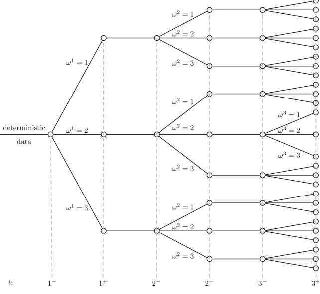
At the beginning of period one, we know nothing apart from the values of the initial (de-terministic) parameters and the structure of the scenario tree with all the corresponding probabilities. The structure of such a scenario tree is depicted in Figure 2. For illustrative purposes we only consider three periods in the planning horizon.
Accordingly, in the beginning of the planning horizon we have to decide which facilities should be set operating in the first period, and which investments and loans to consider in order to maximize the expected profit in the end of period one plus the expected profit in period two. Therefore, the problem we face in the beginning of period one can be stated as follows: max u1,r1,l1 E[Q 1+ (u1,D1(Ω1))] + E[Q2− (r1, l1,ρ2(Ω1))] = max u1,r1,l1 X ω1∈Ω1 P(Ω1 =ω1)·Q1+(u1, D1) + X ω1∈Ω1 P(Ω1 =ω1)·Q2−(r1, l1, ρ2) = max u1,r1,l1 X ω1∈Ω1 P(Ω1 =ω1)·[Q1+ (u1, D1) +Q2−(r1, l1, ρ2)] (1) s.t. M1− X f∈DC Ff1·u1f−X i∈I1 r1i +X i∈B1 l1i ≥0 (2) u1f ∈ {0; 1} ∀f ∈ DC r1i ≥0 ∀i∈ I1 li1≥0 ∀i∈ B1 (3)
The objective function (1) emphasizes our goal of maximizing not only the gain in the end of period 1 but also in the subsequent stages. Equation (2) represents the budget constraint for the first stage. The exogenous budget added to the loans starting in this moment give the available budget for period one which should be spent opening the facilities and eventually making other investments.
deterministic data ω1= 1 ω2= 1 ω2= 2 ω2= 3 ω1= 2 ω2= 1 ω2= 2 ω3 = 1 ω3= 2 ω3= 3 ω2= 3 ω1 = 3 ω2= 1 ω2= 2 ω2= 3 t: 1− 1+ 2− 2+ 3− 3+
Figure 2: Scenario tree with three periods and three events for each period.
End of period 1
Considering the location decisions made in the beginning of period one, as soon as demand is disclosure, we can supply it from the operating facilities. Since we do not know in advance which event will occur (and thus demand and return rates are uncertain), we make this decision dependent on the possible events ω1 ∈Ω1. Moreover, as it was mentioned in section 2 we assume that all the costs and revenues are computed in the end of the time period. The problem we have to solve is the following:
Q1+(u1, D1) = max x1 f,c,p X f∈DC X c∈C X p∈P (R1c,p−Vf,c,p1 )·x1f,c,p·(1 +ROI)T−1 (4)
s.t. X p∈P µp X c∈C x1f,c,p≤K1f·u1f ∀f ∈ DC (5) X p∈P µp X c∈C x1f,c,p≥K1f·u1f ∀f ∈ DC (6) X f∈DC x1f,c,p≤Dc,p1 ∀c∈ C, ∀p∈ P (7) x1f,c,p≥0 ∀f ∈ DC, ∀c∈ C, ∀p∈ P (8)
Constraints (5) and (6) are capacity and minimum throughput constraints. A delivery is possible, if the related facility is operating, but must fall within specified limits. Inequalities (7) limits the deliveries to the amounts demanded by the customers.
Period t∈ {2, ...,T−1}
The reasoning presented above proceeds throughout the planning horizon. At the beginning of thet-th period, the rate of return of the investments of the previous period become known and new operating and investment decision are to be made. Therefor, the following subproblem has to be considered in the beginning of time period t∈ {2, ..., T −1}:
Qt−(r1, ..., rt−1, l1, ..., lt−1, ρt−1) = max ut,rt,ltE[Q t+ (ut,Dt(Ωt))] + E[Q(t+1)−(rt, lt,ρt(Ωt))] = max ut,rt,lt X ωt∈Ωt P(Ωt =ωt)·[Qt+(ut, Dt) +Q(t+1)−(rt, lt, ρt)] (9) s.t. Mt− X f∈DC Fft·utf−X i∈It rti+X i∈Bt lit+ t−1 X τ=1 X i∈Iτ ρti−1·rτi− X i∈Bτ ηti−1·lτi ≥0 (10) utf ∈ {0; 1} ∀f ∈ DC rti ≥0 ∀i∈ It lit≥0 ∀i∈ Bt (11) Taking the decisions made in the beginning of thet-th period (and, consequently, the decisions prior to those), the demand of customers at the end of this period can be satisfied from the operating facilities. So, the subproblem to be solved in the end of period t∈ {2, ..., T −1}
can be generically stated as: Qt+(ut, Dt(ωt)) = max xt f,c,p X f∈DC X c∈C X p∈P (Rtc,p−Vf,c,pt )·xtf,c,p·(1 +ROI)T−t (12) s.t. X p∈P µp X c∈C xtf,c,p≤Ktf·utf ∀f ∈ DC (13) X p∈P µp X c∈C xtf,c,p≥Ktf·utf ∀f ∈ DC (14) X f∈DC xtf,c,p≤Dc,pt ∀c∈ C, ∀p∈ P (15) xtf,c,p≥0 ∀f ∈ DC, ∀c∈ C, ∀p∈ P (16)
Remark 1 Note that subproblem Qt−
(r1, ..., rt−1, l1, ..., lt−1, ρt−1) has to be solved for every
combination of events ω1 ∈Ω1, ..., ωt−1 ∈Ωt−1, while a subproblem Qt+(ut, Dt(ωt)) occurs for every combination of ω1 ∈Ω1, ..., ωt∈Ωt.
Period T
At the beginning of the last period, the structure of the subproblems is still the same:
QT−(r1, ..., rT−1, l1, ..., lT−1, ρT−1) = max uT,rT,lTE[Q T+ (uT,DT(ΩT))] = max uT,rT,lT X ωT∈ΩT P(ΩT =ωT)·QT+(uT, DT) (17) s.t. MT − X f∈DC FfT ·uTf − X i∈IT rTi + X i∈BT lTi + T−1 X τ=1 X i∈Iτ ρTi−1·rτi − X i∈Bτ ηiT−1·liτ ≥0 (18) uTf ∈ {0; 1} ∀f ∈ DC rTi ≥0 ∀i∈ IT liT ≥0 ∀i∈ BT (19)
The subproblems that refer to the end of the planning horizon become enlarged according to: QT+(uT, DT) = max xT f,c,p,αc,d X f∈DC X c∈C X p∈P (RTc,p−Vf,c,pT )·xTf,c,p+X c∈C βc·αc+γ·d + T X τ=1 X i∈Iτ ρTi ·riτ− X i∈Bτ ηTi ·lτi (20) s.t. d≥1− P t∈T P i∈It ρT i ·rti− P i∈Bt ηT i ·lti+ P f∈DC P c∈C P p∈P (Rt c,p−Vf,c,pt )·xtf,c,p·(1 +ROI)T −t P t∈T Mt ·(1 +ROI)T−t+1 (21) X p∈P µp X c∈C xTf,c,p≤KTf ·uTf ∀f ∈ DC (22) X p∈P µp X c∈C xTf,c,p≥KTf ·uTf ∀f ∈ DC (23) X f∈DC xTf,c,p≤Dc,pT ∀c∈ C, ∀p∈ P (24) X t∈T X f∈DC X p∈P xTf,c,p≥αc X t∈T X p∈P Dc,pt ∀c∈ C (25) xTf,c,p≥0 ∀f ∈ DC, ∀c∈ C, ∀p∈ P αc∈[0; 1] ∀c∈ C d≥0 (26)
The objective function (20) contains additional terms concerning the final interest rates, the service level and the downside risk. Beside the capacity constraints (22) and (23), and the restriction on demand (24), we have to consider inequality (21), that restricts the downside risk to the rate we missed the target return on investment for the money we got from our investors. Constraints (25) determine the service level for each customer on the whole time horizon.
Remark 2 SubproblemsQT−(r1, ..., rT−1, l1, ..., lT−1, ρT−1), at the beginning of periodT, has to be solved for every combination of eventsω1 ∈Ω1, ..., ωT−1 ∈ΩT−1, whileQT+(uT, DT(ωT)) occurs for every combination of ω1 ∈Ω1, ..., ωT ∈ΩT.
In comparison to most of the multi-stage stochastic models which have been considered in the literature so far, all variables in all periods somehow interact and it is not possible to reformulate this problem and to solve it recursively (e.g. using dynamic programming). In
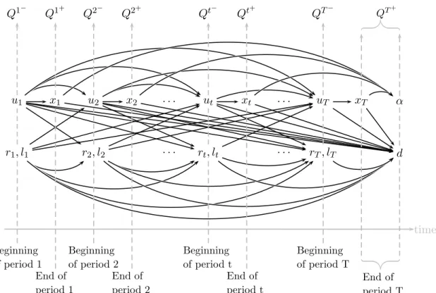
u1 r1, l1 x1 u2 r2, l2 x2 · · · · · · ut rt, lt xt · · · · · · uT rT, lT xT α d time Beginning of period 1 Q1− End of period 1 Q1+ Beginning of period 2 Q2− End of period 2 Q2+ Beginning of period t Qt− End of period t Qt+ Beginning of period T QT− End of period T QT+
Figure 3: Interactions between variables and stages.
order to get a deeper understanding of the relationships between the different stages and variables, they are depicted in Figure 3.
The location decisions immediately determine the delivery decisions in the next stage. Furthermore, they will, together with the investment decisions, limit the available money for all the subsequent location and investment decisions. The service level, at the end of the time horizon is based upon the delivery decisions throughout the planning horizon. The downside risk depends on all decisions made from beginning to end but excluding the service level. Our model does not consider explicitly any non-anticipativity constraints. However, since any decision made in some stage will be fixed for every event (and decisions related with these events), the variables implicitly comprise the non-anticipativity principle. This inhibits an immediate decomposition of SCN DM SF R into deterministic subproblems, one for each scenario.
Since location variables (and therefore integer variables) appear in stages beyond the first, the objective function becomes a weighted average of non-convex, non-differentiable functions. This will prevent any straightforward adaptation of existing solution algorithms for two-stage stochastic linear programming. For instance, a nested Benders decomposition is not achievable (see Carøe and Schultz [6] and Mitra et al. [25] for further details).
Note that we are dealing with a problem which does not have fixed recourse. In fact, for instance in the budget constraints we find random coefficients associated with the decision variables associated with the investments.
Regrettably, most of our decision variables appear in constraints associated to multiple stages and interact with the decisions therein. As we saw, the constraints defining the down-side risk and the service-level comprise decisions for all stages and make it impossible to pull some of the variables together into an aggregated first stage, while some detailed level decisions may be put into a second stage.
Although not having fixed recourse, SCN DM SF R has complete recourse because every feasible solution for a subproblem has a feasible completion in the following stages. This is a feature that may be advantageous from a computational point of view.
The extensive form of this problem formulation may be helpful to makeSCN DM SF R more manageable and to gather more information about it. The interested reader can find this formulation in appendix A.
4
Path-based formulation
The formulation presented so far toSCN DM SF R has the great advantage of clearly highlight-ing the structure of the problem and the relations between the different decisions involved. In this section we propose a more compact formulation to the problem which makes it more suited for being implemented and being handled by a general solver. Furthermore, this formu-lation will be more appropriate to develop special algorithms which take the special structure of the problem into account. The new formulation we propose is based upon the paths in the scenario tree.
St=Ω1 ×Ω2 ×...×Ωt : Set of potential sequences of events until period
t ∈ T. ( ˆ= Set of paths in the scenario tree from the root node to a node in periodt.)
st∈St= (ω1, ..., ωt) : Path of events from the root node to one particular node in period t.
s0 : Root node (e.g. initial situation).
sT : Path of events from the root node to a leaf node,
e.g. a scenario.
pathst ={s0, s1, . . . st} : Set of all (sub)paths sτ (τ ≤ t) which are part of
the pathst.
P(St =st) : Probability that the sequence of events will lead us through the pathst.
I′ =I ∪ B : This will be the set of investments available which now also comprise loans.
I′t=It∪ Bt : Set of investments available in periodt∈ T. r′t
i(st−1) : Amount of money spent or obtained (depending on the case) in investment i ∈ I′t given that the set of events occurring until the beginning of period
t∈ T is defined by path st−1.
r′t(st−1) = ri′t∈I′t(st−1)
r′= (r′1(s0), ..., r′T(sT−1))
ιti : Interest rate of an investment i∈ I′τ, τ ≤t, that has to be paid in the end of periodt∈ T.
u= (u1(s0), ..., uT(sT−1))
x= (x1(s1), ..., xT(sT))
Gtf,c,p : Unitary profit for shipping one unit of productp∈ P from facility f ∈ DC to customerc∈ C in period
t∈ T. This value is considered reported to the end of the planning horizon.
A : Total exogenous budget reported to the end of the
planning horizon.
According to the definitions we have:
P(St =st) = t
Y
τ=1
Gtf,c,p= (Rtc,p−Vf,c,pt )·(1 +ROI)T−t, p∈ P, f ∈ DC, c∈ C, t∈ T (28) A= T X t=1 Mt·(1 +ROI)T−t+1 (29)
Considering the new notation as well as much information presented in the previous section, we can now formulate the problem as follows:
max u,r′,x,α,d X t∈T X st∈St P(St =st)· X f∈DC X c∈C X p∈P Gtf,c,p·xtf,c,p(st) + X sT∈ST P(ST =sT)· X c∈C βc·αc(sT) +γ·d(sT) +X t∈T X st−1∈path sT X i∈I′t ιTi+1(sT)·r′it(st−1) (30) s.t. M1− X f∈DC Ff1·u1f(s0)− X i∈I′1 ri′1(s0)≥0 Mt− X f∈DC Fft·utf(st−1)− X i∈I′t r′it(st−1) + t−1 X τ=1 X i∈I′τ ιit(st−1)·ri′τ(sτ−1)≥0 ∀t∈ T \ {1}, ∀st−1 ∈ St−1, sτ ∈path st−1 A·d(sT)≥A−X t∈T X i∈I′t ιiT+1(sT)·ri′t(st−1) + X f∈DC X c∈C X p∈P Gtf,c,p·xtf,c,p(st) ∀sT ∈ ST, st ∈ path sT X t∈T X f∈DC X p∈P xtf,c,p(st)≥αc(sT) X t∈T X p∈P Dtc,p(st) ∀sT ∈ST, ∀c∈ C, st∈pathsT X p∈P µp X c∈C xtf,c,p(st)≤Ktf ·utf(st−1) ∀t∈ T, ∀st∈St, ∀f ∈ DC, st−1 ∈path st X p∈P µp X c∈C xtf,c,p(st)≥Ktf ·utf(st−1) ∀t∈ T, ∀st∈St, ∀f ∈ DC, st−1 ∈path st X f∈DC xtf,c,p(st)≤Dc,pt (st) ∀t∈ T, ∀st∈St, ∀c∈ C, ∀p∈ P utf(st−1)∈ {0; 1} ∀t∈ T, ∀st−1 ∈St−1, ∀f ∈ DC
r′it(st−1)≥0 ∀t∈ T, ∀st−1 ∈St−1, ∀i∈ I′t xtf,c,p(st)≥0 ∀t∈ T, ∀st∈St, ∀f ∈ DC, ∀c∈ C, ∀p∈ P
αc(sT)∈[0; 1] ∀c∈ C, ∀sT ∈ST
d(sT)≥0 ∀sT ∈ST Not only is this formulation more compact than the one presented in the previous section but also it is more attractive for developing specially tailored procedures for SCN DM SF R. For instance, by relaxing the appropriate sets of constraints we may easily split the problem into different scenarios or into different time periods.
5
The relevance of using a stochastic approach
One important issue arising when a stochastic programming approach is considered for an optimization problem under uncertainty regards the evaluation of the advantages of consid-ering such approach in comparison with more ‘simplified’ methodologies. With this purpose, we propose that the optimal value of a deterministic problem derived from the stochastic one is considered as explained below.
Assume, that all the data are given, as described in the sections above. If the problem should be model as a deterministic problem, one would have to compute the expected inter-est rates E[ιti(St)] and expected demands E[Dc,pt (St)], first. Afterwards, the deterministic
problem can be formulated according to: max u,r,x,α,d X t∈T X f∈DC X c∈C X p∈P Gtf,c,p·xtf,c,p+X c∈C βc·αc+γ·d+ X t∈T X i∈I′t E[ιti(St)]·r′it (31) s.t. M1− X f∈DC Ff1·u1f − X i∈I′1 r′i1≥0 Mt− X f∈DC Fft·utf − X i∈I′t r′it+ t−1 X τ=1 X i∈I′τ E[ιti(St)]·ri′τ ≥0 ∀t∈ T \ {1} A·d≥A−X t∈T X i∈I′t E[ιti(St)]·ri′t+ X f∈DC X c∈C X p∈P Gtf,c,p·xtf,c,p
X t∈T X f∈DC X p∈P xtf,c,p≥αc X t∈T X p∈P E[Dc,pt (St)] ∀c∈ C X p∈P µp X c∈C xtf,c,p≤Ktf ·utf ∀t∈ T, ∀f ∈ DC X p∈P µp X c∈C xtf,c,p≥Ktf ·utf ∀t∈ T, ∀f ∈ DC X f∈DC xtf,c,p≤E[Dc,pt (St)] ∀t∈ T, ∀c∈ C, ∀p∈ P utf ∈ {0; 1} ∀t∈ T, ∀f ∈ DC r′it≥0 ∀t∈ T, ∀i∈ I′t xtf,c,p≥0 ∀t∈ T, ∀f ∈ DC, ∀c∈ C, ∀p∈ P αc ∈[0; 1] ∀c∈ C d≥0
Naturally, the result of this problem can not immediately be compared with the stochastic so-lution. In fact the delivery-decisions may provide more than the costumers’ demands and the investment decisions may budget too much or not enough money, so that not all constraints will be satisfied in every scenario. Additionally, the deterministic model may underestimate the downside-risk.
For these reasons, one can use the model above to set the location and investment decisions and adapt the transportation decisions and additional investment decisions, as soon as the real demands and interest rates become known.
In doing so, we solve SCN DM SF R with fixed location and investment decisions again, but al-low investing additional money in the worst investment and adapt the optimal transportation decisions for all scenarios. In our opinion, the objective value of this approach is a realistic deterministic equivalent to the stochastic solution.
Once we have solved the deterministic problem, we consider the relative value of the multi-stage stochastic solution (RV M S) with respect to the deterministic solution as a measure of the relevance of using a stochastic approach:
RV M S = Q
M SS−QDET
QDET . (32)
QDET denotes the optimal objective value of the deterministic problem (more precisely of the stochastic problem with fixed location and investment decisions) and QM SS the optimal value of the multi-stage stochastic program.
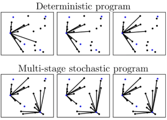
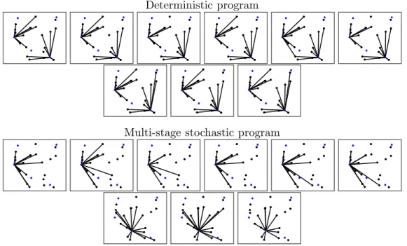
In order to receive an impression about how different the solutions provided by the multi-stage stochastic programming approach and by the deterministic one may be, we present the results for one instance of a small problem with 3 periods, 5 potential locations, 20 customers, 8 investments and three stochastically independent events for each period. In total we have 27 different scenarios. All data are generated as it is described in appendix B. First, we do not allow loans and interpret the results. This allow us to focus our attention on the location decisions. The results of this case are depicted in Figures 4, 5 and 6. Afterwards, we will add the possibility of loans to this instance and solve it again in order to highlight the importance of softening the common usage of fixed budget constraints.
Deterministic program
Multi-stage stochastic program
Figure 4: Example, period 1, no loans
In this example, the stochastic solution tends to open more facilities and to satisfy more de-mand in the first period (Figure 4). This is because forecast uncertainty for dede-mand increases ,and so the variation in the optimal location decisions for individual scenarios decreases, in time. It is obvious that investment decisions also change based on this observation.
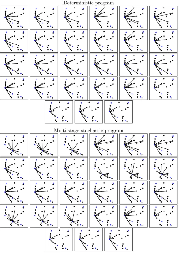
In the deterministic problem, most of the demand will be satisfied in the second stage, since the expected demand, that can be reached in this period is (by choice) higher than in the other periods. It must be pointed out that the higher variability in this period has no impact on the deterministic decision, but on the stochastic one, were less facilities are located in this uncertain environment (Figure 5).
In both approaches only one DC is opened in the third period, but there is also a difference remarkable (Figure 6). The deterministic approach will always open the same facility, since this one guarantees the highest expected profit. In contrast, the stochastic approach will open one of two different facilities, depending on the scenario, and so depending on the demand
Deterministic program
Multi-stage stochastic program
Figure 5: Example, period 2, no loans
which we have already satisfied and the profit which we have already made.
The objective value of the multi-stage stochastic model isQM SS= 184658, while the objective value of the deterministic problem is QDET = 182561. Thus,
RV M S= 184658−182561
182561 = 1.149%.
Note that the objective value of the deterministic model before adapting the transportation and investment decisions to the scenarios is 184537. It overestimates the real objective value, that can be reached by its location decisions, by 1.08%.
Assume now that we have also loans available. In particular we consider 3 loans. The deterministic solution does not change, because the expected rates of the investments are below the rates of the loans (otherwise, the problem will lead to a trivial solution) and it is (by choice) not profitable to open an additional facility with this additional money. The stochastic model takes advantage of some loans and combines them with some investments with different durations. In doing so, the available budget increases and the location decisions change (two and in some scenarios even three facilities will be opened in period two and three). Therefore a much higher objective value can be reached (QM SS = 203747) and the relative value of the multi-stage stochastic solution increases significantly: RV M S = 11.605%.
Deterministic program
Multi-stage stochastic program
Figure 6: Example, period 3, no loans
6
Computational Results
In order to evaluate the possibility of solving SCN DM SF R, we run a series of computational tests.
We considered the more compact formulation presented for the problem i.e., the path-based formulation proposed in the previous section. The model was implemented using the C++ optimization modeling library and interface ILOG Concert Technology. A variety of test problems was solved with ILOG CPLEX 11.2, on a Intel Core 2 PC with two 1.86 GHz processors and 2GB RAM. Single-core computing was used.
We consider problem instances with T = 3 periods, 5 potential locations, 20 customers, 8 different investments (that vary in their duration), returns and variability. Furthermore, we consider 3 different loans, each of them starting at the beginning of a different period. We considered three and nine stochastically independent events for each period, respectively which led to |ST |= 27 and |ST |= 729 scenarios, respectively. In the first case, instances with 3623 constraints and 9265 variables (56000 non-zeros on average and 65 binary variables) were obtained. In the second situation we got instances with 56441 constraints and 172574 variables (more than 1.3 million non-zeros and 455 binary variables).
We generated n= 300 instances for the 27 scenario-case andn= 30 for the 729 scenario case. Details concerning the generation of the data can be found in B.
For all instances, not onlySCN DM SF Rwas considered but also the deterministic problem associated as described in the previous section. The computation time consist not only of the time to solve the problem, but also of the time to create the model. In all tests, a time limit of three hours was considered.
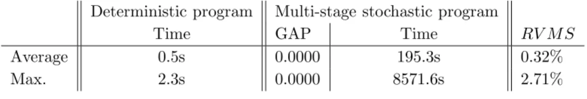
The computational results of all instances are summarized in Table 1 for the 27 scenario-case and Table 2 for the 729 scenario-scenario-case, respectively. As described below, we were not able to solve every instance of the multi-stage stochastic program within the time limit. Therefore, we report the GAP after three hours. RV M S denotes the relative value of the stochastic solution, as it is discussed in section 5. If we were not able to compute the optimal solution within the time limit, the best solution we found so far is used to compute this value.
Deterministic program Multi-stage stochastic program
Time GAP Time RV M S
Average 0.5s 0.0000 195.3s 0.32%
Max. 2.3s 0.0000 8571.6s 2.71%
Table 1: Results, |ST |= 27
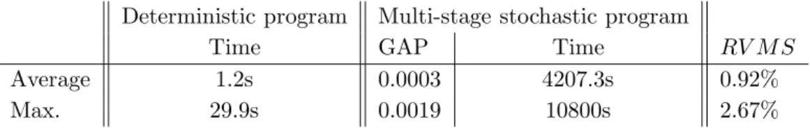
As expected, the computation times for the multi-stage stochastic program are much higher than in the deterministic case. Anyhow, we were able to solve all instances with 27 scenarios in less than three hours. In the considerably larger case of 729 scenarios, 22 of 30 instances were solved within the time limit. The GAP is smaller than 0.05% in 5 of the
Deterministic program Multi-stage stochastic program
Time GAP Time RV M S
Average 1.2s 0.0003 4207.3s 0.92%
Max. 29.9s 0.0019 10800s 2.67%
Table 2: Results,|ST |= 729
remaining 8 instances and less than 0.2% in the worst 3 cases.
The solution, found within the time limit, was better than the optimal solution of the deter-ministic model in 245 of 300 and all cases, respectively. The improvement was higher than 1% in 17 cases and almost higher than 2% in 4 cases of the 27 scenario instances. 15 of 30 instances with 729 scenarios improved the deterministic solution more than 1% and in 2 cases even more than 2%. As a result, we can summarize, that a remarkable improvement can be achieved, if multi-stage stochastic aspects are considered in SCND. If real-world instances are too large to ensure finding the optimal solution with standard solvers like CPLEX, in reasonable time, it is possible to find good feasible solutions, which adapt much better to the future than deterministic models do.
7
Conclusion
In this paper, a supply chain network design problem was studied. In addition to common decisions in these type of problems we included financial decisions with relevance for a com-pany managing a supply chain. The goal is to maximize the net financial benefit. Revenues were taken into account as well as a target for the return on investment and a risk measure associated with the possibility of falling below that target. Due to the uncertainty in the demand the service level is measured and included in the objective function. A mixed-integer multi-stage stochastic programming formulation was proposed. The deterministic equivalent was presented as well as an alternative formulation based upon the paths in the scenario tree. The relevance of considering stochasticity was discussed and illustrated with a small example. The computational results obtained using a set of randomly generated instances show that the modeling framework proposed in this paper is promising for dealing with multi-period supply chain network design problems. Moreover, the computational results also open good perspectives in terms of the development of more comprehensive models. Regarding the methodologies for solving these type of problems new directions are also opened with this work.
A
Extensive Form
max u1,...,uT,r1,...,rT,l1,...,lT,x1 f,c,p,...,xTf,c,p,αc,d X ω1∈Ω1 P(Ω1 =ω1)· X f∈DC X c∈C X p∈P (Rc,p1 −Vf,c,p1 )·x1f,c,p·(1 +ROI)T−1 + X ω2∈Ω2 P(Ω2 =ω2)· X f∈DC X c∈C X p∈P (R2c,p−Vf,c,p2 )·x2f,c,p·(1 +ROI)T−2+. . . + X ωt∈Ωt P(Ωt =ωt)· X f∈DC X c∈C X p∈P (Rc,pt −Vf,c,pt )·xtf,c,p·(1 +ROI)T−t+. . . + X ωT∈ΩT P(ΩT =ωT)· X f∈DC X c∈C X p∈P (Rc,pT −Vf,c,pT )·xTf,c,p +X c∈C βc·αc+γ·d+ T X τ=1 X i∈Iτ ρTi ·riτ− X i∈Bτ ηTi ·lτi . . . (33) s.t. M1− X f∈DC Ff1·u1f −X i∈I1 r1i +X i∈B1 li1≥0 M2− X f∈DC Ff2·u2f −X i∈I2 r2i +X i∈B2 li2+X i∈I1 ρ1i ·ri1− X i∈B1 ηi1·l1i ≥0 ∀ω1∈Ω1 .. . MT − X f∈DC FfT ·uTf − X i∈IT riT + X i∈BT liT + T−1 X τ=1 X i∈Iτ ρTi −1·rτi −X i∈Bτ ηiT−1·lτi ≥0 ∀ω1 ∈ Ω1, . . . , ∀ωT−1 ∈ΩT−1 d≥1− P t∈T P i∈It ρT i ·rti− P i∈Bt ηT i ·lti+ P f∈DC P c∈C P p∈P (Rt c,p−Vf,c,pt )·xtf,c,p·(1 +ROI)T −t P t∈T Mt ·(1 +ROI)T−t+1 ∀ω1 ∈ Ω1, . . . , ∀ωT ∈ ΩT X t∈T X f∈DC X p∈P xtf,c,p≥αc X t∈T X p∈P Dc,pt ∀c∈ C, ∀ω1 ∈Ω1, . . . , ∀ωT ∈ΩTX p∈P µp X c∈C x1f,c,p≤K1f ·u1f ∀f ∈ DC, ∀ω1 ∈Ω1 X p∈P µp X c∈C x1f,c,p≥K1f ·u1f ∀f ∈ DC, ∀ω1 ∈Ω1 X p∈P µp X c∈C x2f,c,p≤K2f ·u2f ∀f ∈ DC, ∀ω1∈Ω1, ∀ω2 ∈Ω2 X p∈P µp X c∈C x2f,c,p≥K2f ·u2f ∀f ∈ DC, ∀ω1∈Ω1, ∀ω2 ∈Ω2 .. . X p∈P µp X c∈C xTf,c,p≤KTf ·uTf ∀f ∈ DC, ∀ω1 ∈Ω1, . . . , ∀ωT ∈ΩT X p∈P µp X c∈C xTf,c,p≥KTf ·uTf ∀f ∈ DC, ∀ω1 ∈Ω1, . . . , ∀ωT ∈ΩT X f∈DC x1f,c,p≤Dc,p1 ∀c∈ C, ∀p∈ P, ∀ω1 ∈Ω1 X f∈DC x2f,c,p≤Dc,p2 ∀c∈ C, ∀p∈ P, ∀ω1∈Ω1, ∀ω2 ∈Ω2 .. . X f∈DC xTf,c,p≤Dc,pT ∀c∈ C, ∀p∈ P, ∀ω1 ∈Ω1, . . . , ∀ωT ∈ΩT αc ∈[0; 1] ∀c∈ C, ∀ω1 ∈Ω1, . . . , ∀ωT ∈ΩT d≥0 ∀ω1 ∈Ω1, . . . , ∀ωT ∈ΩT u1f ∈ {0; 1} ∀f ∈ DC r1i ≥0 ∀i∈ I1 li1≥0 ∀i∈ B1 x1f,c,p≥0 ∀f ∈ DC, ∀c∈ C, ∀p∈ P, ∀ω1 ∈Ω1 u2f ∈ {0; 1} ∀f ∈ DC, ∀ω1 ∈Ω1 r2i ≥0 ∀i∈ I2, ∀ω1 ∈Ω1 li2≥0 ∀i∈ B2, ∀ω1 ∈Ω1
x2f,c,p≥0 ∀f ∈ DC, ∀c∈ C, ∀p∈ P, ∀ω1∈Ω1, ∀ω2 ∈Ω2 .. . uTf ∈ {0; 1} ∀f ∈ DC, ∀ω1 ∈Ω1, . . . , ∀ωT−1∈ΩT−1 rTi ≥0 ∀i∈ I3, ∀ω1 ∈Ω1, . . . , ∀ωT−1∈ΩT−1 liT ≥0 ∀i∈ B3, ∀ω1 ∈Ω1, . . . , ∀ωT−1∈ΩT−1 xTf,c,p≥0 ∀f ∈ DC ∀c∈ C, ∀p∈ P, ∀ω1 ∈Ω1, . . . , ∀ωT ∈ΩT
B
Data
The data for the test instances were generated as follows:
• 3 periods.
• 5 potential locations.
• 20 customers.
• 8 investments.
• 0 and 3 loans, respectively.
• 3 and 9 stochastically independent events for each period, respectively.
• The fixed cost for operating a facility are all set to 21000 monetary units per period.
• The transportation costs for product 1 (2) are set to 0.025 (0.05) monetary units per unit and distance unit.
• The customers and the potential facilities are randomly located on a square of (100×100) distance units according to a uniform distribution.
• The unitary revenue of product 1 (2) is set to 2.5 (2.75) monetary units. This revenue is assumed to be equal for every customer and every period.
• Every operating facility has a minuimum throughput of 500 and the maximum capacity is 15000 per period.
• The unit capacity consumption factor of product 1 (2) is 1 (1.5).
• The exogenous budget at the beginning of period 1 is set to 10000, of period 2 to 60000 and of period 3 to 30000.
• The interest rates depend on the duration of the loans and vary between 7.5% and 8.5%.
• In every period, there is always one agreed investment which pays a fixed rate on return. This rate depends on the duration again and varies between 4.5% and 6%. All other investments have uncertain rates on return, which are generated by normal distributions. Depending on their risk, the distributions rage fromN(0.04,0.01) to N(0.065,0.02).
• The target ROI is fixed to 20%.
• The weights are all set to the same value for all customers (unweighted case) and are used just to scale the service level. Therefore, they are set to the sum of exogenous budget divided through the number of customers.
• The weight for the downside risk is set to the sum of exogenous budget.
• Demands are generated according to an auto-regressive processes:
Dt
c,p(St):=Dc,pt−1(St−1)+ε ∀t∈ T \ {1}, with Dc,p1 (S1)∼ LN(7,0.5) andε∼ LN(7,0.5)−0.9·E[Dc,p1 (S1)]. If any realization becomes negative, it is set to zero.
• The probabilities for the events depend on the number of scenarios. They vary between 25% and 50% in the cases of 27 scenarios and between 4% and 22% in the 729 scenario-cases.
References
[1] E. Aghezzaf. Capacity planning and warehouse location in supply chains with uncertain demands. Journal of the Operational Research Society, 56:453–462, 2005.
[2] S. Ahmed. Convexity and decomposition of mean-risk stochastic programs.Mathematical
Programming, 106:433–446, 2006.
[3] S. Ahmed, A. King, and G. Parija. A multi-stage stochastic integer programming ap-proach for capacity expansion under uncertainty. Journal of Global Optimization, 26: 3–24, 2003.
[4] A. Alonso-Ayuso, L. F. Escudero, A. Gar´ın, M. T. Ortu no, and G. P´erez. An ap-proach for strategic supply chain planning under uncertainty based on stochastic 0-1 programming. Journal of Global Optimization, 26:97–124, 2003.