1
Assessing reliability of NDE flaw detection using smaller number of
demonstration data points
Ajay M. Koshti, NASA Johnson Space Center, Houston, U.S.A.
ABSTRACT
The paper provides an engineering analysis approach for assessing reliability of NDE flaw detection using smaller number of demonstration data points. It explores dependence of probability of detection (POD), probability of false positive (POF), on contrast-to-noise ratio, and net decision threshold-to-noise ratio in a simulated data; and draws some generically applicable inferences to devise the approach. ASTM nondestructive evaluation standards provide requirements on signal-to-noise ratio and/or contrast-signal-to-noise ratio in order to provide reliable flaw detection and limit false positive calls. POD analysis of inspection test data results in an estimated flaw size, denoted by 𝑎90/95. This flaw size has 90% POD and minimum 95% confidence. POF is also estimated in the analysis. POD demonstration requires specimens with flaws of known size. In many situations, it is very expensive to produce the large number of flaws required for the POD analysis. In some situations, only real flaws can truly represent the flaws for demonstration. Real flaws of correct size and location in part configuration specimen may be difficult to produce, if not impossible. Here, an engineering analysis approach is devised using simulation to assess reliability of NDE technique when a limited number of flaws are available for demonstration. In this simulation, a technique is considered reliable, if it provides flaw detectability size equal to or better than the theoretical 𝑎90𝑡ℎ used in simulation and also provides a POF less than or equal to a chosen value. The paper uses simulated signal response versus flaw size data to devise the approach. Linear correlation is used between the signal response data and flaw size. POD software mh1823 uses generalized linear model (GLM) in POD analysis after transforming the flaw size and signal response, if needed, using logarithm. Therefore, this approach is in agreement with the linear signal correlation used in mh1823. Using the POD analysis of data, generic conditions on contrast-to-noise ratio and net decision threshold-to-noise ratio are derived for reliable flaw detection. In order to assess technique reliability using the engineering approach, signal response-to-flaw size correlation about the flaw size of concern is needed. In addition, measurement of noise is also needed. If the technique meets the above requirements, assumption of linear signal-to-flaw size correlation and conditions on noise, then the technique can be assessed using this analysis as it fits the underlying POD model used here. The approach is conservative and is designed to provide a larger flaw size compared to the POD approach. Such NDE technique assessment approach, although, not as rigorous as POD, can be cost effective if the larger flaw size can be tolerated. Typically, this is a situation for all quality control NDE inspections. Here, an NDE technique needs to be reliable and 𝑎90/95is not estimated, but the assessed flaw size is assumed to be larger than the unknown a90 due to conservative factors or margins. Applicability of the approach for assessing reliability of flaw detection
in x-ray radiography and 2D imaging in general is also explored.
Keywords: probability of detection, probability of false positive, signal-to-noise ratio, contrast to noise ratio
1. INTRODUCTION
MIL-HDBK-18231 and associated mh18232 software cover two types of datasets. First type of dataset is signal response
â (read as a-hat) versus flaw size “a”. The â (y-axis) versus “a” (x-axis) data may be transformed using logarithm function along appropriate axes, if needed, to create linear fit around the decision threshold level. A generalized linear model (GLM) is fitted to the transformed data for analysis. Here, noise data is taken separately to define noise distribution. Noise is same as signal response from part where there is no flaw. Noise data is used to determine false call rate or probability of false positive calls (POF).
Second type of dataset is called hit-miss data, which contains flaw size and corresponding detection result i.e. hit or miss. Hit has numerical value of 1 and miss has numerical value of 0. Here, false call data is noted to determine POF using Clopper-Pearson binomial distribution function. Normally, POD increases with flaw size and POF decreases with flaw size. POF value shall be within certain limit to prevent adverse impact on cost and schedule. ASTM E 28623 also provides
There are other approaches that are not covered by MIL-HDBK-1823. Point estimate method of verifying reliably detectable flaw size is given by Rummel4. Koshti5 provides an approach for optimizing the point estimate method. A curve
can be fitted to the data as opposed to fitting a straight line using general linear model (GLM) used in MIL-HDBK-1823. The chosen curve shall be based on the physics model or based on demonstration on additional similar inspection data. For signal response type POD analysis, curves with a90/95 upper and lower bounds2 and POF2 as a function of decision
threshold are very useful in optimizing decision threshold.
In signal response POD model, a quantity that relates to detection of the flaw is needed. In X-ray radiography, observed anomaly image contrast from a flaw is the primary flaw detection parameter. A compound X-ray flaw size parameter that relates to flaw image contrast can be derived from a physics based model (Koshti6-9). In infrared flash thermography,
normalized image and temperature contrast of flaw can be used as signal response for POD analysis (Koshti10-16).
Engineering analysis approaches are not considered to be statistical analysis in complying with MIL-HDBK-1823 or point estimate method. Since they do not meet all the necessary requirements for statistical analysis, they may use some conservative margin (Koshti17) to the POD results from a similar inspection case. An engineering analysis approach for
assessment of dye penetrant crack detectability in external corners using crack detection data from surface flaws is provided by Koshti18. Another example of engineering analysis, provided by Koshti19, is estimating reliably detectable
flaw size for NDE methods, such as eddy current testing, that use technique calibration. Here, decision threshold level versus a90/95 curves are used for transferring calibration sensitivity established on electro-discharge machined (EDM)
notches for detection of cracks. In another engineering analysis example, Koshti20 provides eddy current crack detection
capability assessment approach using crack specimens with different electrical conductivity. Engineering approaches for flaw size assessment shall be approved by responsible engineering board. Koshti21 validates the approach given in this
paper using Monte Carlo simulation of sample data. Koshti22 develops NDE flaw estimation using smaller number of
hit-miss data-points. The approach is validated using Monte Carlo sampling. Although, the approach is developed using simulation, the approach probably could be developed based on theory of statistics.
2. SIMULATION APPROACH
This approach is based on hypothesis that simulated data used in 𝑎̂ versus “a” curve-fit POD or 𝑎̂ versus “a” mh1823 POD analysis can be used to devise necessary conditions for engineering analysis for assessment of NDE technique reliability. Therefore, if POD methods are used to determinate POD curves, perform noise analysis, choose decision threshold, and perform POF analysis, then this information can be used to devise the necessary conditions for the engineering analysis. The following linear signal response versus flaw size model is used. Signal response 𝑎̂ relates to flaw size “a”as follows.
𝑎̂ = 𝛽1𝑎 + 𝛽0+ 𝛿, (1)
where, 𝛽0 and 𝛽1are constants. Although a linear relationship is chosen, other relationships as given in MIL-HDBK-1823 also apply. Noise δ is assumed to have Normal distribution with constant standard deviation σ. First, a symmetrical POD function curve based on error function (erf) is chosen. This is given by cumulative density distribution of a probability density function, which is chosen to be a Normal distribution. This meets the key assumption that POD increases with flaw size. Probability density function (PDF), in the form of Normal distribution, is given by,
𝑓(𝑎) = 1
𝜎∗√2𝜋𝑒 −(𝑎−𝜇)2
2𝜎∗2 . (2)
POD function is given by cumulative density distribution function (CDF) of the Normal distribution function PDF. It is given by,
𝑔(𝑎, 𝜇, 𝜎∗ ) = 1
2[1 + 𝑒𝑟𝑓 ( 𝑎−𝜇
𝜎∗√2)], (3)
where, 𝜇 is mean of the PDF and CDF functions at a given decision threshold. 𝜎 and 𝜎* are standard deviations of noise δ and for PDF (or CDF) function at a given decision threshold respectively. 90% POD is given by following expression,
0.9 = 𝑔(1.2815, 0, 1). Following CDF expression from Matlab may be used.
𝑔(𝑎) = 0.5[1 + 𝑒𝑟𝑓(𝐶1𝑎 − 𝐶2)], (4)
where,
𝐶2= 𝜇 𝜎⁄ ∗√2. (6) From Eq. 5, we can calculate the standard deviation in POD model as,
𝜎∗= √2𝐶
1. (7)
From Eq. 6, mean used is calculated as,
𝜇 = 𝐶2𝜎∗√2. (8)
Following signal response model was used to generate data.
𝑎̂ = 10𝑎 + 5 + 𝛿. (9)
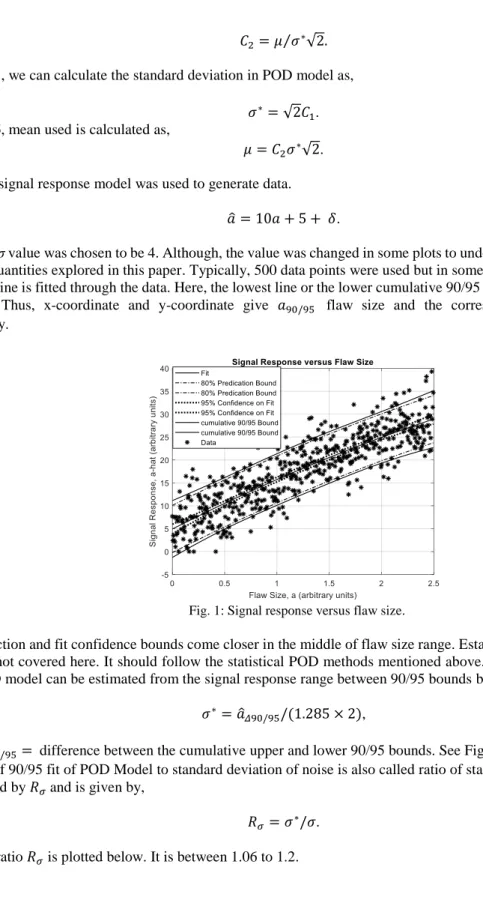
Typically, σ value was chosen to be 4. Although, the value was changed in some plots to understand how value of σ affects the other quantities explored in this paper. Typically, 500 data points were used but in some plots the number was varied. A straight line is fitted through the data. Here, the lowest line or the lower cumulative 90/95 bound is same as the decision threshold. Thus, x-coordinate and y-coordinate give 𝑎90/95 flaw size and the corresponding decision threshold respectively.
Fig. 1: Signal response versus flaw size.
Data prediction and fit confidence bounds come closer in the middle of flaw size range. Establishing POD and confidence bounds is not covered here. It should follow the statistical POD methods mentioned above. Apparent standard deviation of the POD model can be estimated from the signal response range between 90/95 bounds by,
𝜎∗= 𝑎̂
𝛥90/95/(1.285 × 2), (10)
where 𝑎̂𝛥90/95= difference between the cumulative upper and lower 90/95 bounds. See Fig. 1. Ratio of standard
deviation of 90/95 fit of POD Model to standard deviation of noise is also called ratio of standard deviation of noise here. It is denoted by 𝑅𝜎and is given by,
𝑅𝜎= 𝜎∗/𝜎. (11)
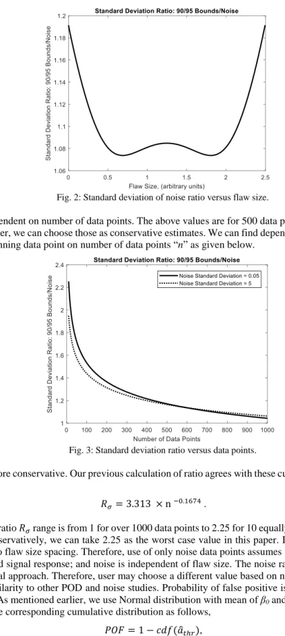
Fig. 2: Standard deviation of noise ratio versus flaw size.
Noise ratio 𝑅𝜎 is dependent on number of data points. The above values are for 500 data points. Since the values for ends in above plot are higher, we can choose those as conservative estimates. We can find dependency of the standard deviation of noise ratio of beginning data point on number of data points “n” as given below.
Fig. 3: Standard deviation ratio versus data points.
The upper curve is more conservative. Our previous calculation of ratio agrees with these curves. Fit equation for the upper curve is given below.
𝑅𝜎= 3.313 × n −0.1674. (12)
Notice that the noise ratio 𝑅𝜎 range is from 1 for over 1000 data points to 2.25 for 10 equally distributed data points around target flaw size. Conservatively, we can take 2.25 as the worst case value in this paper. If only noise measurements are made, then there is no flaw size spacing. Therefore, use of only noise data points assumes that there is a linear correlation between flaw size and signal response; and noise is independent of flaw size. The noise ratio 𝑅𝜎 is the only conservative factor in this empirical approach. Therefore, user may choose a different value based on number of data points or choose a value based on similarity to other POD and noise studies. Probability of false positive is calculated using a probability density distribution. As mentioned earlier, we use Normal distribution with mean of β0 and standard deviation of 𝜎∗. POF is calculated using the corresponding cumulative distribution as follows,
where 𝑎̂𝑡ℎ𝑟= signal decision threshold level.
Next we compute various signal-to-noise and decision threshold-to-noise ratios. If noise is measured as standard deviation, 𝑛𝜎 then it is given by,
𝑛𝜎 = 𝜎∗. (14)
If noise is measured as 90% percentile or as cumulative noise,
𝑛90= 1.285 𝜎∗. (15)
Average signal response is given by 𝑎̂𝑚. This would require multiple measurements at a given target flaw size and average of these measurements can be taken as 𝑎̂𝑚 for flaw size 𝑎𝑚. Curve for signal response 𝑎̂𝑚 versus flaw size am is shown
by fit curve in Fig. 1. Noise can be measured as standard deviation of these measurements but the flaw size must be same. Else, it is recommended to get noise measurements in the vicinity of a demonstration test flaw to be detected. Noise measurements in region outside flaw area provide mean as β0 and standard deviation as σ. β0 is considered to be baseline signal response and not noise. Contrast is given by,
𝑐 = 𝑎̂𝑚− 𝛽0. (16)
Decision threshold 𝑎̂𝑡ℎ𝑟= 𝑎̂90/95. See Fig. 1. Net decision threshold is given by,
𝑎̂𝑡ℎ𝑟_𝑛𝑒𝑡= 𝑎̂𝑡ℎ𝑟− 𝛽0. (17) Using the assumed POD model (Eq. (3)), a condition for POD > 90% based on relative contrast ratio 𝐶𝑟𝑒𝑙𝑁𝑅, is given
below.
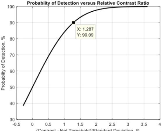
𝐶𝑟𝑒𝑙𝑁𝑅=((𝑎̂𝑚− 𝛽0)−(𝑎̂𝑡ℎ𝑟− 𝛽0))/𝜎∗ ≥ 1.285. (18) If average signal from a certain size flaw and noise meet the above condition, termed merit ratio Condition 1, then that flaw can be detected reliably if POF is acceptable. Condition 1 is shown below in Fig. 4.
Fig. 4: Probability of detection versus relative contrast ratio.
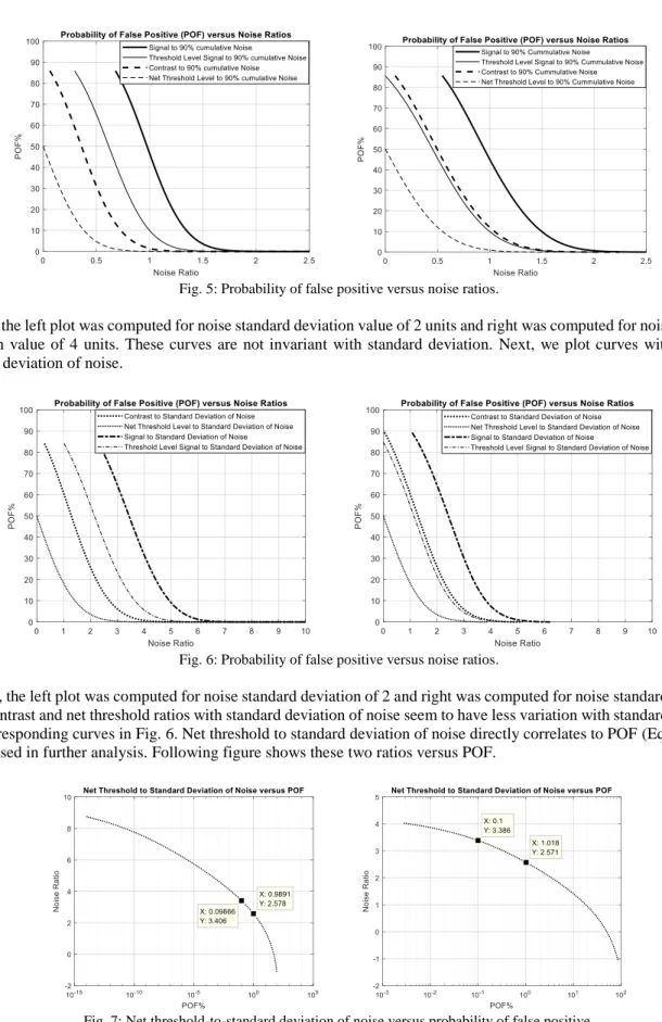
Further noise analysis is required for estimating POF. First, we plot ratios with cumulative noise and their relationship with POF is calculated using Eq. (13).
Fig. 5: Probability of false positive versus noise ratios.
In Fig. 5 the left plot was computed for noise standard deviation value of 2 units and right was computed for noise standard deviation value of 4 units. These curves are not invariant with standard deviation. Next, we plot curves with ratios to standard deviation of noise.
Fig. 6: Probability of false positive versus noise ratios.
In Fig. 6, the left plot was computed for noise standard deviation of 2 and right was computed for noise standard deviation of 4. Contrast and net threshold ratios with standard deviation of noise seem to have less variation with standard deviation than corresponding curves in Fig. 6. Net threshold to standard deviation of noise directly correlates to POF (Eq. (13)) and will be used in further analysis. Following figure shows these two ratios versus POF.
In Fig. 7, the left figure was computed for noise standard deviation of 2 and right was computed for noise standard deviation of 4. We assume that POF = 0.1% is reasonable. Later, we will also use 1% POF. The corresponding ratios are annotated in above figures. Given few points of noise data with standard deviation σ, we need to compute minimum contrast-to-noise ratio, minimum threshold-to-contrast-to-noise ratio and minimum contrast-to-net threshold ratio. Standard deviation of contrast-to-noise for the 90/95 bounds is given by,
𝜎∗= 𝑅
𝜎𝜎. (19)
Conservative value for the standard deviation ratio can be taken as 2.25 corresponding to n = 10.
𝑅𝜎= 2.25. (20)
From Fig. 6, contrast-to-standard deviation of noise ratio (CNR) is calculated as follows,
𝐶𝑁𝑅 = (𝑎̂𝑚− 𝛽0)/𝜎 = 𝑅𝜎× 4.67 = 2.25 × 4.67 = 10.5. (21) Merit ratio Condition 2A: Contrast-to-standard deviation of noise ratio, CNR ≥ 10.5. From Fig. 7, Net threshold-to-standard deviation of noise (TNR) is computed as follows,
𝑇𝑁𝑅 = (𝑎̂𝑡ℎ𝑟− 𝛽0)/𝜎 = 𝑅𝜎× 3.4 = 2.25 × 3.4 = 7.65. (22) Merit ratio Condition3A: Net threshold-to-standard deviation of noise, 𝑇𝑁𝑅 ≥ 7.65. We use net noise i.e. noise about the baseline. An approximate way of calculating 99 percentile net noise in Normal distribution is,
𝑛99𝑛𝑒𝑡= 2.36 × 𝑅𝜎𝜎. (23)
Therefore, contrast-to-net noise ratio is given by,
(𝑎̂𝑚− 𝛽0)/𝑛99𝑛𝑒𝑡= 4.45. (24) Merit ratio Condition 2B: Contrast-to-net noise ratio ≥ 4.45. Also net threshold-to-net noise ratio is given by,
(𝑎̂𝑡ℎ− 𝛽0)/𝑛99𝑛𝑒𝑡= 3.24 (25) Merit ratio Condition 3B: Net threshold-to-net noise ≥ 3.24.
𝐶𝑇𝑅 = 𝐶𝑁𝑅 𝑇𝑁𝑅⁄ = (𝑎̂𝑚− 𝛽0) (𝑎̂⁄ 𝑡ℎ𝑟− 𝛽0). (26) Merit ratio Condition 4: Contrast-to-net threshold ratio (CTR) should be approximately ≥ 1.37 for 1% POF. Threshold shall be set to 71% of the average flaws size amplitude. Lower decision threshold is better but conditions on contrast and threshold-to-noise ratios values shall also be met. This condition may have lower ratios as we simply took ratio of CNR and TNR to establish an approximate value21.
Condition 1 (Eq. (18)) is an assumption of The POD model and is used to set the decision threshold values. It uses the assumed value of noise ratio. Accuracy of the 𝑎̂𝑚 will depend upon number of flaw responses averaged. Noise ratio of 2.25 was assumed to be good for 10 flaws. Condition 1 is used to determine decision threshold with assumed value of noise ratio for a chosen sample size for flaws. It sets the values of CNR, TNR and CTR.
Condition 2 on CNR is necessary to ensure that Conditions 3 and 4 would be met. CNR primarily influences POD. See Fig. 4.
Condition 3 on TNR primarily influences POF. See Fig. 7. Condition 4 on CTR influences both POD and POF.
It is postulated that in addition to affirming 𝑎̂ versus a linearity with constant noise, when the three Conditions, i.e. 2, 3, and 4, as given in Table 1 are met, then the instance of flaw detection is considered to be reliable detection.
Conditions 2, 3, and 4 can be further validated through Monte Carlo simulation21. Koshti21 provides refinement of Table
1 conditions by lowering the merit ratio values by using lower 𝑅𝜎 noise ratio and providing minimum required values for the CTR.
These engineering rule of thumb or cook-book conditions can be used, if conventional POD analysis could not be performed. The same analysis is performed for POF = 1%. Results of POF values of 0.1% and 1% are summarized below.
Table 1: Conditions for reliable flaw detection, noise ratio = 2.25
Condition Description Abbreviation POF = 0.1% POF = 1% Change
1 Difference in contrast and net threshold normalized to standard deviation of 90/95 bounds, Eq. (18)
CrelNR ≥1.285 ≥1.285 0
2A Contrast-to-standard deviation of noise ratio, Eq. (21)
CNR ≥ 10.5 ≥ 8.66 1.845
2B Contrast-to-net noise ratio, Eq. (24) CNR ≥ 4.45 ≥ 3.67 0.78
3A Net threshold-to-standard deviation of noise, Eq. (22)
TNR ≥ 7.65 ≥ 5.76 1.89
3B Net threshold-to-net noise, Eq. (25) TNR ≥ 3.24 ≥ 2.44 0.8
4 Ratio of the contrast-to-net threshold ratio, Eq. (26) CTR ~1.37 ~1.5 -0.13
Last column gives difference between the columns 3 and 4. Higher POF of 1% allows lower merit ratios almost by 1 unit for ratios based on net noise and by 2 units for ratios based on standard deviation of noise. CTR is increased by 9% as POF is increased to 1%. Therefore, greater separation is needed between the indication contrast and decision threshold for POF of 1%. This is understandable as overall merit ratios for POF of 1% are lower.
Minimum signal-to-noise ratio (equivalent to contrast-to-net noise ratio in Table 1) of 3 is commonly used, which is in agreement with numbers given in Condition 2B. For expensive hardware, all indications, i.e. true positive or false positive, are further evaluated using another NDE method. Therefore, POF of 1% may be economically viable. The above analysis is applicable for single-hit detection such as in ultrasonic testing using only A-scan display or eddy current testing using only impedance plane display.
3. APPROACH FOR ASSESSING TECHNIQUE RELIABILITY IN X-RAY RADIOGRAPHY
Only volumetric flaws will be considered here. Detection of tight cracks (Koshti6-9) is excluded in this analysis. Here, we
will only consider a few measured metrics from the above analysis and other factors such as resolution and contrast sensitivity. Correlation of indication shape and size with corresponding flaw shape and size is not considered here. Other factors such as scatter radiation, x-ray reflection at grazing angles (Koshti8) and beam hardening will not be addressed.
When inspection results are presented in a C-scan or 2D image, flaw image size i.e. length and width also affect POD and POF. 3D image data obtained in x-ray Computed Tomography (CT) can be evaluated as a 2D slice image. If smallest or target flaw size to be detected is mapped in a grid or cluster of 3 by 3 (3 x 3) resolution pixels, then the above requirements need to be applied to the cluster of 3 x 3 resolution pixels. Here, each side of the square pixel is equal to the estimated resolution or total unsharpness per ASTM E2698.
Consider x-ray digital radiography (DR) with rigid panel. Assume that the linear flaw response model is applicable. In digital radiography, typically, minimum contrast-to-noise ratio of 2.5 is needed in the relevant image quality indicator (IQI) hole per ASTM E2698–10, para. 10.19.3.2. Here, flaw size, that is to be reliably detected, is same as the relevant penetrameter hole size. If this analysis is used for qualification, then the noise level should be about same between the qualification testing and actual inspection. If probability of detecting a single pixel size flaw is 𝑃𝑂𝐷𝑖, then probability of flaw detection in (3x3) cluster, PODm is given by,
𝑃𝑂𝐷𝑚= 1 − (1 − 𝑃𝑂𝐷𝑖)𝑁, (27)
where, PODm = POD for the pixel cluster and 𝑃𝑂𝐷𝑖= POD for individual pixel. N = number of pixels in the cluster, i.e. 9 in this case. Note that above equation is also valid for linear indication of a flaw. The above equation assumes that the signal is independent of flaw size or modulation transfer function (MTF) of the cluster is 1. This assumption is valid if we assume that the signal registered by each pixel is about same as average signal of the cluster of 3 x 3 pixels. Thus, if
𝑃𝑂𝐷𝑖= 23%, then POD of 3 x 3 cluster 𝑃𝑂𝐷𝑚= 90% using Eq. (27). However, 𝑃𝑂𝐷𝑖 cannot be lower than 50%. If 𝑃𝑂𝐷𝑖 < 50%, decision threshold is set above the average contrast, which is wrong. It is assumed that the net threshold shall not exceed the average contrast. With this assumption, the limiting case of net threshold is when threshold is equal to average contrast. Here, 𝑃𝑂𝐷𝑖 of individual pixel is 50% and for 3 x 3 cluster of resolution size pixels, 𝑃𝑂𝐷𝑚= 99.8% using Eq. (27). This value meets the minimum 0.9 requirement for POD. The following calculation used noise standard deviation value of 4 units.
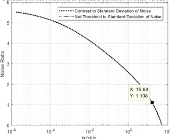
Fig. 9: Contrast and net threshold-to-standard deviation of fit noise versus probability of false positive.
sensitivity is needed in a cluster of 3 x 3 pixels of size equal to the resolution, which may be modulated to modulation transfer function (MTF) value of, for example, 80%. Therefore, contrast sensitivity needed on void indication will be higher,
𝐶𝑆3𝑥3= 𝐶𝑆/𝑀𝑇𝐹3𝑥3= 2/0.8 = 2.5%. (28)
See Fig. 10.
Fig. 10: Boundary of image of round void or hole of IQI and 3 x 3 cluster of resolution size pixels.
The contrast sensitivity is like 99 percentile noise. For Normal noise distribution,
𝑛99= 2.36𝜎. (29)
Therefore, standard deviation of noise in terms of percent thickness t is,
100 𝜎⁄ =𝑡 𝐶𝑆3𝑥3% 2.36 =
2.5%
2.36 =1.06%. (30)
ASTM E2737 uses a value of 2.5 instead of 2.36 with a similar approach. Therefore, minimum contrast sensitivity at void needed to meet contrast-to-noise ratio of 2.5 is given by,
𝐶𝑆𝑣𝑜𝑖𝑑=
𝐶𝑁𝑅×𝐶𝑆 (2.36𝑀𝑇𝐹3𝑥3)=
2.5×2%
2.36×0.8= 2.65%. (31)
The above equation implies that, given CS = 2%, contrast sensitivity for detection of void needs to be raised to 2.65%. Estimated resolution or total unsharpness Ulm per ASTM E2698 is given by,
𝑈𝑙𝑚 = 1 𝜈√(𝑈𝑔) 3 + (1.6 𝑆𝑅𝑏)3 3 and, (32) 𝑈𝑔= (𝜈 − 1)ø, (33)
where Ug is geometric unsharpness. ν is the largest geometric magnification present in the image which happens at
maximum distance of point on object from detector. Ø is the x-ray source focal spot size per ASTM E1165 and the detector
basic resolution SRb is calculated using method specified in ASTM E2597. Thus, the flaw is mapped in 3Ulm x 3Ulm. See
Fig. 10. The assumption of minimum 80% MTF would be valid for this flaw size. Thus, for digital radiography, a void with minimum thickness 2.65% of the total thickness and a size of 3Ulm x 3Ulm would be detected with 𝑃𝑂𝐷𝑖𝑚 as previously calculated to be 99.8%. Let us calculate the POF of the cluster.
A point of 15.68% POF (net threshold-to-standard deviation of noise ratio = 1.1) is noted on the plot and is chosen for analysis. This point gives with 𝑃𝑂𝐷𝑖= 50% and as previously calculated 𝑃𝑂𝐷𝑚= 99.8%. This point was chosen so that contrast-to-standard deviation of noise ratio (CNR) is 2.5 when decision threshold is same as average contrast.
𝐶𝑁𝑅 = (𝑎̂𝑡ℎ𝑟− 𝛽0)/𝜎 = 2.25 × 1.1 = 2.5. (34)
For this point, the POF for 3 x 3 resolution size pixel grid is given by 𝑃𝑂𝐹𝑚 ,
where 𝑃𝑂𝐹𝑚 = POF for pixel cluster and 𝑃𝑂𝐹𝑖= POF for individual pixels. N = number of pixels in a cluster, i.e. 9 in this case. POF for a cluster of 3 x 3 resolution size pixel cluster is negligible. Note that above equation is also valid for a linear indication of a flaw. ASTM E27367 recommends minimum seven effective pixels covering the longest dimension of defect.
The above analysis assumes a decision threshold based flaw detection where decision threshold is same as average contrast. This is good for automated flaw detection. However, for visual flaw detection, detection criteria is simply visible contrast from the noise.
Fig. 11: Signal and noise at CNR = 2.5.
Fig. 11 shows Normal probability density distributions for signal and noise for CNR = 2.5. Standard deviation for predicted signal response is higher. See Eq. 19. For visual detection, the decision threshold is likely to be between the crossing of the two distributions i.e. at signal response of 6.37 units in Fig. 11 and the average signal response is 7.5 units. Here, we consider the worst POD case of visual flaw detection with decision threshold at the crossing point i.e., athr = 6.37 units.
Threshold at crossing point provides a false call rate of 8.5% and POD of 69.2% for a single pixel using Eq. (4) and (13) respectively. CNR = 2.5 is measured in 3 x 3 resolution pixel grid. Therefore, using Eq. (27), for 9 pixels, the POD is 96.4%. This POD is lower than 99.8% which was previously calculated for decision threshold at average contrast level. But visually detected flaw size is smaller than that detected by using decision threshold as average signal response of a target flaw. Using Eq. (35), POF is ~0 for the decision threshold level at the crossing point. Thus, for visual detection also, the detection for CNR = 2.5 is reliable.
Fig. 12: Simulated CNR = 10 in left image and CNR = 2.5 in right image. One 3 x 3 cluster indication in top left and two 7 x 1 linear indications.
Fig. 12 shows simulated images for 3 x 3 pixel cluster and two 7 x 1 linear indications with CNR = 10 and CNR = 2.5. The images confirm that the indications are visually detectable at CNR = 2.5. As expected, reliability of flaw detection in 2D imaging or multi-hit detection is much higher compared to that in single-hit detection using real time A-scan signal for the same contrast-to-noise ratio. Typically, in digital radiography, using rigid detector array, detector basic resolution SRb is related to the detector pixel size by,
where, d = detector pixel size. Therefore, using Eq. 31, the minimum Ulm = 1.28 x d,which is approximately same as SRb.
Typically, a pore is round with lateral dimension same as pore thickness. Diameter of pore is 1.414 times the 3 x 3 pixel grid width. This is illustrated in Fig. 10. The figure shows a circle representing the pore edge and the inscribed square box accommodates a grid of 3 x 3 resolution size pixels. Since contrast sensitivity, CS is a measure of noise-to-signal ratio, signal-to-noise ratio in acreage can be calculated as,
𝑆𝑁𝑅 = 100 × 2.36/𝐶𝑆 (37)
ASTM E2737 uses a value of 2.5 instead of 2.36.
𝑆𝑁𝑅 ≥ 100 × 2.5/𝐶𝑆 (38)
Thus, using Eq. (38) minimum SNR in acreage is calculated as 125 for CS of 2% and 250 for CS of 1%. In para. 10.19.3.4, ASTM E2698 states, if the CNR of the IQI is not accessible, alternatively the signal-to-noise ratio (SNR) shall be measured in an area of homogeneous gray level in the unprocessed image. The SNR shall exceed 130 for 2 % contrast sensitivity and exceed 250 for 1 % contrast sensitivity.
Thus, diameter of round pore that is reliably detected is 3 x 1.414 Ulm = 4.2Ulm. Using Eq. (31), maximum thickness of
material that can be inspected using contrast sensitivity of 2% would be,
𝑡𝑚𝑎𝑥 = (100 × 4.2 × 𝑈𝑙𝑚) 𝐶𝑆⁄ 𝑣𝑜𝑖𝑑. = 4.2 x 100 x Ulm. /2.65 = 160 Ulm. (39)
Normally, parts are much thinner. Thus, for detection of round pores, flaw detectability is controlled by the lateral dimension of pore, not by its thickness. For resolution Ulm of 0.002”, detectable pore diameter is 0.0084”. Maximum
material thickness is 0.32” for this pore, provided Ulm is maintained at this thickness.
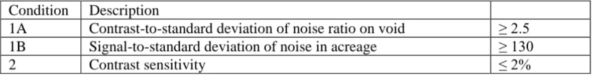
Table 2: Conditions for reliably detecting 4.2 x Ulm diameter void with minimum 2.65% thickness.
Condition Description
1A Contrast-to-standard deviation of noise ratio on void ≥ 2.5 1B Signal-to-standard deviation of noise in acreage ≥ 130
2 Contrast sensitivity ≤ 2%
Conditions 1A and 1B are redundant to each other. The above model is also applicable to detection of round inclusions. Signal response is assumed to be linear with material density difference between a flaw and surrounding homogeneous material in x-ray digital radiography including rigid panel digital radiography (DR), flexible phosphor plate computed radiography (CR) and computed tomography (CT). The contrast sensitivity is inversely proportional to density difference 𝛥𝜌 as,
𝐶𝑆𝑖𝑛𝑐𝑙𝑢𝑠𝑖𝑜𝑛≅ 𝐶𝑆𝑣𝑜𝑖𝑑 𝛥𝜌𝑣𝑜𝑖𝑑
𝛥𝜌𝑖𝑛𝑐𝑙𝑢𝑠𝑖𝑜𝑛. (40)
Note that for void or gas porosity, density difference is between the part material and air (or gas); and for inclusion it is between inclusion material and part material. If x-ray film is digitized, then above analysis is valid, provided transformed flaw response is linear with thickness change and noise is constant. Eq. (32) is applicable for film radiography, if film SRb is measured. Normally, one may assess the SRb qualitatively evaluating film radiograph of line pair gage. This value will not be as accurate. Assuming film SRb > 0 in Eq. (32), we get following requirement for film radiography,
𝑈𝑙𝑚 > 𝑈𝑔
𝜈. (41)
Similarly, for the volumetric flaw of size a, we have following requirement,
𝑎 𝑈𝑙𝑚
⁄ > 4.2. (42)
𝑎𝜈 𝑈𝑔
⁄ > 4.2. (43)
Resolution Ulm is applicable to the 2D imaging in radiography and it is assumed to be measured where flaws can occur and the chosen location is the worst location from flaw detectability point of view.
In cone beam x-ray CT using rigid panel detectors, resolution can be measured from part edge response, line pair gage on or inside a simulated part, or by using a simulated part with rows of holes with different sizes. Simulated parts with known flaws are called representative quality indicator (RQI). ASTM E1817 provides requirements for use of RQI. We would assume that x-ray CT data is analyzed as 2D slice images. Detection of flaws in multiple neighboring parallel slices passing through the anomaly indication increases POD. We have an equation for POD that is similar to Eq. (27). Here, P1,P2 ….Pi are PODs in each slice where flaw is detected. Here, i is number of independent parallel slices detecting the anomaly. The slice thickness is assumed to be at least equal to the local resolution at flaw location. The composite POD of detecting flaws in multiple slices is higher than that in each slice. The composite POD is given by,
𝑃𝑂𝐷𝑚= 1 − (1 − 𝑃𝑂𝐷1)(1 − 𝑃𝑂𝐷2) … . . (1 − 𝑃𝑂𝐷𝑖). (44) Eq. (44) is also the generic equation for multi-point POD. Detection of flaw in multiple slices reduces POF. We have an equation for POF that is similar to Eq. (35). The composite POF is given by,
𝑃𝑂𝐹𝑚= 𝑃𝑂𝐹1𝑃𝑂𝐹2. . . . 𝑃𝑂𝐹𝑖. (45)
Eq. (45) is also the generic equation for multi-point POF. Here, we can determine localized resolution near flaw location. This resolution is measured in the part using RQI as opposed to calculating it, and is equivalent to Ulmin the above analysis. It can be measured as a line pair gap or wire size providing MTF value of 0.2 and is interpolated from MTF versus line pair frequency (line-pair/mm) response curve. There are limits on x-ray CT resolution. Given source size s and detector pixel size d, the best possible resolution R occurs at a particular value of geometric magnification ν and the quantities are given by, 𝜈𝑏𝑒𝑠𝑡= 𝑑 𝑠+ 1, 1 𝑈𝑏𝑒𝑠𝑡= 1 𝑠+ 1 𝑑 (46)
Thus, best possible resolution value is smaller than the smallest between the detector pixel size and source size. In microfocus x-ray CT, the detector pixel size may be an order larger than focal spot. In such situation, the resolution is approximately ~90% of source size. Resolution is controlled by detector size for low magnification and is given by,
𝜈 < 𝜈𝑏𝑒𝑠𝑡, 𝑈𝑚𝑎𝑥 = 𝑑
𝜈. (47)
Resolution is controlled by source size for high magnification and is given by,
𝜈 ≥ 𝜈𝑏𝑒𝑠𝑡, 𝑈𝑚𝑎𝑥= (1 − 1
𝜈) 𝑠. (48)
In order to get above resolution, sufficient number of shots are needed. For 360 degree rotation in cone beam x-ray CT, recommended number of shots Nshots is given by,
𝑁𝑠ℎ𝑜𝑡𝑠= 𝜋
2𝑛𝑝𝑖𝑥𝑒𝑙, (49)
where, npixel = number of pixels, along an axis normal to rotation axis, needed to image the object in the scan. Although, this is a recommended value, part density variation, geometry, scattering, beam hardening, and distance from rotation axis would also affect the resolution. Choice of x-ray energy (kV) and filters are also important to make sure that signal response is not saturated or is insufficient to provide linear correlation of signal response with material thickness. Since x-ray CT has a volume pixel or voxel, depth resolution relates to contrast sensitivity. Normally, a cubical voxel is used with size
above analysis is also applicable to x-ray CT. It is believed that reliability of x-ray NDE techniques for volumetric flaws can be assessed, to some extent, based on measurements on small number of flaws in all worst locations from detection point of view using the above analysis approach.
Similarly, it is postulated that in other 2D imaging NDE methods, where linear model for transformed signal response and flaw size is applicable, the above analysis is also applicable. It is recommended to measure resolution using relevant resolution targets including RQI. Using same approach, reliability of flaw detection in other 2D imaging NDE methods can also be assessed, to some extent, based on measurements on small number of flaws in all worst locations.
4. CONCLUSIONS
Engineering analysis rule of thumb or cook-book conditions are given based on analysis of simulated data to assess reliability of an NDE technique. The approach assumes linear correlation between signal and flaw size. Noise is assumed to have constant standard deviation. Assessment of reliability of x-ray radiography NDE, including film, DR, CR and CT, is also considered. This approach is also applicable to assessment of reliability of flaw detection in other 2D imaging techniques. The analysis indicates that, multi-hit detection in 2D pixel cluster to image flaw is inherently more reliable than using just single-hit detection similar to that using only real time A-scan signal display. The approach uses ratio of standard deviation of noise as a factor to control conservatism in the assessment. Therefore, user may choose a different value than suggested here based on number of demonstration data points or based on similarity to other POD studies. Minimum 10 data points are recommended in signal correlation and noise measurements. The approach is conservative and is designed to provide a larger flaw size compared to the POD approach. Such NDE technique assessment engineering approach, although, not as rigorous as POD can be cost effective, if higher flaw size can be tolerated. Typically, this situation occurs for all quality control NDE inspections. For quality control, NDE technique needs to have consistent sensitivity but a90/95 flaw size is not estimated. The assessed flaw size in this analysis has high confidence that it is larger
than the unknown true a90 due to conservative factors used in the analysis.
5. ACKNOLEDGEMENTS
William Prosser (NASA Langley Research Center, NASA Engineering Safety Center - NESC), Floyd Spencer (NESC), David Stanley (NASA Johnson Space Center), Ron Beshears (NASA Marshall Space Flight Center - MSFC), and James Walker (NASA MSFC) provided valuable review comments to this work.
REFERENCES
[1] MIL-HDBK-1823A, “Nondestructive Evaluation System Reliability Assessment,” Department of Defense, USA, (2009).
[2] Annis, Charles, “mh1823 POD Software V5.2.1,” Statistical Engineering, http://www.statisticalengineering.com/mh1823/, (2016).
[3] ASTM E 2862-12, “Standard Practice for Probability of Detection for Hit/Miss Data,” ASTM International, (2012). [4] Rummel Ward D., “Recommended Practice for Demonstration of Nondestructive Evaluation (NDE) Reliability on
Aircraft Production Parts,” Materials Evaluation, August Issue 40 pp 922, (1988).
[5] Koshti, A. M., Optimizing probability of detection point estimate demonstration”, Nondestructive Characterization and Monitoring of Advanced Materials, Aerospace, and Civil Infrastructure, Proc. of SPIE Vol. 10169, (2017). [6] Koshti, A. M., “Modeling the X-ray Process and X-ray Flaw Size Parameter for POD Studies,” Proc. SPIE 9063,
Nondestructive Characterization for Composite Materials, Aerospace Engineering, Civil Infrastructure, and Homeland Security, (2014).
[7] Koshti, A. M., “Simulating the X-ray Image Contrast to Set-up Techniques with Desired Flaw Detectability,” Structural Health Monitoring and Inspection of Advanced Materials, Aerospace, and Civil Infrastructure, Proc. of SPIE Vol. 9437, (2015).
[8] Koshti, A. M., “Crack detection flaw size parameter modeling for x-rays at grazing angle to crack faces”, Nondestructive Characterization and Monitoring of Advanced Materials, Aerospace, and Civil Infrastructure, Proc. of SPIE Vol. 10169, (2017).
[9] Koshti, A. M., “X-ray ray tracing simulation and flaw parameters for crack detection,” SPIE Smart Structures and NDE, Proc. of SPIE Vol. 10600, (2018).
[10] Koshti, A. M., “Methods and Systems for Characterization of an Anomaly Using Infrared Flash Thermography,” National Aeronautics and Space Administration, U.S. Patent US8577120 B1, (2013).
[11] Koshti A.M., “Flash Infrared Thermography Contrast Data Analysis Technique,” NASA Technical report server, http://ntrs.nasa.gov, Doc. ID. 20140012757, NASA Tech Briefs Webinar; Meeting Sponsor, NASA Johnson Space Center; Houston, TX, (2014).
[12] Koshti, A. M., “Infrared Contrast Analysis Technique for Flash Thermography Nondestructive Evaluation, Document ID: 20140012756, Report/Patent Number: AK3-14, JSC-CN-32013; Patent US 8,577,120, Technical Reporthttps://ntrs.nasa.gov/, (2014).
[13] Koshti, A. M., “Measuring and Estimating Normalized Contrast in Infrared Flash Thermography,” NASA Technical report server, http://ntrs.nasa.gov, Doc. ID: 20130009802, NASA Tech Brief, NASA Johnson Space Center; Houston, TX, United States (2013).
[14] Koshti, A. M., “Infrared Contrast Data Analysis Method for Quantitative Measurement and Monitoring in Flash Infrared Thermography,” Structural Health Monitoring and Inspection of Advanced Materials, Aerospace, and Civil Infrastructure 2015, edited by Peter J. Shull, Proc. of SPIE Vol. 9437, 94370X-2, www.spie.org, San Diego, (2015). [15] Koshti, A. M., “Methods and Systems for Measurement and Estimation of Normalized Contrast in Infrared
Thermography,” National Aeronautics and Space Administration, US Patent US 9,066,028 B1, (June 23, 2015). [16] Koshti, A. M., “Normalized Temperature Contrast Processing in Infrared Flash Thermography,” SAMPE Long
Beach, (2016).
[17] Koshti, A. M., “Applicability of a Conservative Margin Approach for Assessing NDE Flaw Detectability,” Aging Aircraft 2007 Palm Springs CA, http://ntrs.nasa.gov/, (2007).
[18] Koshti, A. M., “Assessment of dye penetrant crack detectability in external corners using similarity analysis,” SPIE Smart Structures and NDE, Proc. of SPIE Vol. 10599, (2018).
[19] Koshti, A.M., “Reliably detectable flaw size for NDE methods that use calibration”, Nondestructive Characterization and Monitoring of Advanced Materials, Aerospace, and Civil Infrastructure, Proc. of SPIE Vol. 10169, (2017). [20] Koshti, A. M., “Eddy current crack detection capability assessment approach using crack specimens with differing
electrical conductivity,” SPIE Smart Structures and NDE, Proc. of SPIE Vol. 10599, (2018).
[21] Koshti, A. M., “NDE flaw detectability validation using smaller number of signal response data-points”, NASA Technical Report Server, http://ntrs.nasa.gov, NASA Johnson Space Center, (2018).
[22] Koshti, A. M., “NDE flaw estimation using smaller number of hit-miss data-points”, NASA Technical Report Server, http://ntrs.nasa.gov, NASA Johnson Space Center, (2018).