Subset Basis Approximation of Kernel Principal Component Analysis

Selection of our books indexed in the Book Citation Index in Web of Science™ Core Collection (BKCI)

Interested in publishing with us?

Contact [email protected]

For more information visit www.intechopen.com Open access books available

Countries delivered to _{Contributors from top 500 universities}

International authors and editors

Our authors are among the

most cited scientists

Downloads

We are IntechOpen,

the world’s leading publisher of

Open Access books

Built by scientists, for scientists

12.2%

122,000

135M

TOP 1%

154

Subset Basis Approximation of Kernel

Principal Component Analysis

Yoshikazu Washizawa

1. Introduction

Principal component analysis (PCA) has been extended to various ways because of its simple definition. Especially, non-linear generalizations of PCA have been proposed and used in various areas. Non-linear generalizations of PCA, such as principal curves (Hastie & Stuetzle, 1989) and manifolds (Gorban et al., 2008), have intuitive explanations and formulations comparing to the other non-linear dimensional techniques such as ISOMAP (Tenenbaum et al., 2000) and Locally-linear embedding (LLE) (Roweis & Saul, 2000).

Kernel PCA (KPCA) is one of the non-linear generalizations of PCA by using the kernel trick (Schölkopf et al., 1998). The kernel trick nonlinearly maps input samples to higher dimensional space so-called the feature space F. The mapping is denoted by Φ_{, and let} x

be ad-dimensional input vector,

Φ _:Rd _{→ F, x→}Φ₍x). (1) Then a linear operation in the feature space is a non-linear operation in the input space. The dimension of the feature space_F is usually much larger than the input dimensiond, or could be infinite. The positive definite kernel functionk(·,·)that satisfies following equation is used to avoid calculation in the feature space,

k(x1,x2) =Φ(x1),Φ(x2) ∀x1,x2∈Rd, (2)

where_·,_·denotes the inner product.

By using the kernel function, inner products in F are replaced by the kernel function k : Rd_×Rd _→ R_{. According to this replacement, the problem in F is reduced to the problem} inRn_{, where n is the number of samples since the space spanned by mapped samples is at} mostn-dimensional subsapce. For example, the primal problem of Support vector machines (SVMs) in_F is reduced to the Wolf dual problem inRn_{(Vapnik, 1998).}

In real problems, the number ofn is sometimes too large to solve the problem in Rn_{. In the} case of SVMs, the optimization problem is reduced to the convex quadratic programming whose size isn. Even ifn is too large, SVMs have efficient computational techniques such as chunking or the sequential minimal optimization (SMO) (Platt, 1999), since SVMs have sparse solutions for the Wolf dual problem. After the optimal solution is obtained, we only have to store limited number of learning samples so-called support vectors to evaluate input vectors.

In the case of KPCA, the optimization problem is reduced to an eigenvalue problem whose size is n. There are some efficient techniques for eigenvalue problems, such as the divide-and-conquer eigenvalue algorithm (Demmel, 1997) or the implicitly restarted Arnoldi method (IRAM) (Lehoucq et al., 1998)1. However, their computational complexity is still too large to solve whennis large, because KPCA does not have sparse solution. These algorithms requireO(n2)working memory space andO(rn2)computational complexity, wherer is the number of principal components. Moreover, we have to store all n learning samples to evaluate input vectors.

Subset KPCA (SubKPCA) approximates KPCA using the subset of samples for its basis, and all learning samples for the criterion of the cost function (Washizawa, 2009). Then the optimization problem for SubKPCA is reduced to the generalized eigenvalue problem whose size is the size of the subset, m. The size of the subset m defines the trade-off between the approximation accuracy and the computational complexity. Since all learning samples are utilized for its criterion, even ifmis much smaller thann, the approximation error is small. The approximation error due to this subset approximation is discussed in this chapter. Moreover, after the construction, we only have to store the subset to evaluate input vectors.

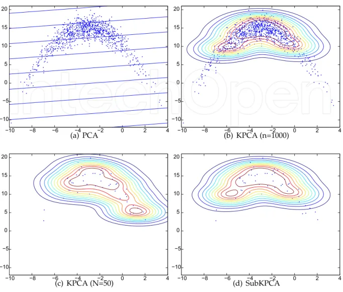
An illustrative example is shown in Figure 1. Figure 1 (a) shows artificial 1000 2-dimensional samples, and contour lines of norms of transformed vectors onto one-dimensional subspace by PCA. Figure 1 (b) shows contour curves by KPCA (transformed to five-dimensional subspace in _F). This is non-linear analysis, however, it requires to solve an eigenvalue problem whose size is 1000. For an input vector, calculations of kernel function with all 1000 samples are required. Figure 1 (c) randomly selects 50 samples, and obtains KPCA. In this case, the size of the eigenvalue problem is only 50, and calculations of kernel function with only 50 samples are required to obtain the transform. However, the contour curves are rather different from (b). Figure 1 (d) shows contour curves of SubKPCA by using the 50 samples for its basis, and all 1000 samples for evaluation. The contour corves are almost that same with (b). In this case, the size of the eigenvalue problem is also only 50, and the number of calculations of kernel function is also 50.

There are some conventional approaches to reduce the computational complexity of KPCA. improved KPCA (IKPCA) (Xu et al., 2007) is similar approach to SubKPCA, however, the approximation error is much higher than SubKPCA. Experimental and theoretical difference are shown in this chapter. Comparisons with Sparse KPCAs (Smola et al., 1999; Tipping, 2001), Nyström method (Williams & Seeger, 2001), incomplete Cholesky decomposition (ICD) (Bach & Jordan, 2002) and adaptive approaches (Ding et al., 2010; Günter et al., 2007; Kim et al., 2005) are also diecussed.

In this chapter, we denote vectors by bold-italic lower symbolsx,y, and matrices by bold-italic capital symbols A,B. In kernel methods, F could be infinite-dimensional space up to the selection of the kernel function. If vectors could be infinite (functions), we denote them by italic lower symbols f,g. If either domain or range of linear transforms could be infinite-dimensional space, we denote the transforms by italic capital symbols X,Y. This is summarized as follows; (i) bold symbols,x,A, are always finite. (ii) non-bold symbols, f,X, could be infinite.

í10 í5 0 5 10 15 20 í10 í8 í6 í4 í2 0 2 4 (a) PCA í10 í5 0 5 10 15 20 í10 í8 í6 í4 í2 0 2 4 (b) KPCA (n=1000) í10 í5 0 5 10 15 20 í10 í8 í6 í4 í2 0 2 4 (c) KPCA (N=50) í10 í5 0 5 10 15 20 í10 í8 í6 í4 í2 0 2 4 (d) SubKPCA

Fig. 1. Illustrative example of SubKPCA

2. Kernel PCA

This section briefly reviews KPCA, and shows some characterizations of KPCA.

2.1 Brief review of KPCA

Let x₁, . . . ,xn be d-dimensional learning samples, and X = [x1|. . .|xn] ∈ Rd×n.

Suppose that their mean is zero or subtracted. Standard PCA obtains eigenvectors of the variance-covariance matrixΣ_, Σ₌1 n n

∑

Then the ith largest eigenvector corresponds to the ith principal component. Suppose

U_PCA = [u_1|. . .|ur]. The projection and the transform ofx ontor-dimensional eigenspace

In the case of KPCA, input vectors are mapped to feature space before the operation. Let S =[Φ₍x₁)_|. . ._|Φ₍xn)] (4)

Σ_{F =SS}∗ ₍₅₎

K =S∗S ∈Rn×n_{, (6)} where _·∗ denotes the adjoint operator2, andK is called the kernel Gram matrix (Schölkopf et al., 1999), andi,j-component ofK isk(x_i,x_j). Then theith largest eigenvector corresponds to the ith principal component. If the dimension of F is large, eigenvalue decomposition (EVD) cannot be performed. Let{λi,ui}be theith eigenvalue and corresponding eigenvector

ofΣ_F respectively, and_{λi,vi}be theith eigenvalue and eigenvector ofK. Note thatKand

Σ_F have the same eigenvalues. Then theith principal component can be obtained from the ith eigenvalue and eigenvector ofK,

ui = √1

λi

Sv_i. (7)

Note that it is difficult to obtain ui explicitly on a computer because the dimension of F

is large. However, the inner product of a mapped input vector Φ₍x) and the ith principal component is easily obtained from,

u_i,Φ(x)= _√1

λi

v_i,kx, (8)

kx= [k(x,x1), . . . ,k(x,xn)]⊤ (9)

kxis ann-dimensional vector called the empirical kernel map.

Let us summarize using matrix notations. Let

Λ_{KPCA =diag([λ1, . . . ,λr]) (10)}

UKPCA = [u1|. . .|ur] (11)

V_KPCA = [v_1|. . ._|vr]. (12)

Then the projection and the transform ofxonto ther-dimensional eigenspace are

UKPCAUKPCA∗ Φ(x) =SVKPCAΛ−1VKPCA⊤ kx, (13)

U_KPCA∗ Φ₍x) =Λ−1/2_V⊤

KPCAkx. (14)

2.2 Characterization of KPCA

There are some characterizations or definitions for PCA (Oja, 1983). SubKPCA is extended from the least mean square (LMS) error criterion3.

min X J0(X) = 1 n n

∑

2_{In real finite dimensional space, the adjoint and the transpose·}⊤ _{are equivalent. However, in infinite}

dimensional space, the transpose is not defined

3_{Since all definitions of PCA lead to the equivalent solution, SubKPCA is also defined by the other} definitions. However, in this chapter, only LMS criteria is shown.

From this definition, X that minimizes the averaged distance between x_i and Xx_i overi is obtained under the rank constraint. Note that from this criterion, each principal component is not characterized, i.e., the minimum solution isX =U_PCAU_PCA⊤ , and the transformU_PCA is not determined.

In the case of KPCA, the criterion is min X J1(X) = 1 n n

∑

where _R(A) denotes the range or the image of the matrix or the operator A, and _N(A) denotes the null space or the kernel of the matrix or the operator A. In linear case, we can assume that the number of samples n is sufficiently larger than r and d, and the second constraint N(X) ⊃ R(S)⊥ is often ignored. However, since the dimension of the feature space is large,rcould be larger than the dimension of the space spanned by mapped samples

Φ_{(x1), . . . ,}Φ_{(xn). For such cases, the second constraint is introduced.}

2.2.1 Solution to the problem (16)

Here, brief derivation of the solution to the problem (16) is shown. Since the problem is in R(S),Xcan be parameterized byX =SAS∗,A_∈Rn×n_{. Accordingly, J1yields}

J₁(A) = 1 nS−SAS ∗_S2 F = 1 nTrace[K−KAK−KA ⊤_K+A⊤_KAK] = 1 nKAK 1/2_−K1/22 F (17)

where _·1/2 denotes the square root matrix, and _· F denotes the Frobenius norm. The

eigenvalue decomposition of K is K = ∑n_i=1λiviv_i⊤. From the Schmidt approximation

theorem (also called Eckart-Young theorem) (Israel & Greville, 1973),J1is minimized when

KAK1/2 = r

∑

∑

2.3 Computational complexity of KPCA

The procedure of KPCA is as follows; 1. CalculateKfrom samples. [O(n2)]

2. Perform EVD for K, and obtain the r largest eigenvalues and eigenvectors, λ1, . . . ,λr,

v₁, . . .vr. [O(rn2)]

3. ObtainΛ−1/2_V⊤

KPCA, and store all training samples.

4. For an input vectorx, calculate the empirical kernel mapkxfrom Eq. (9). [O(n)]

The procedures 1, 2, and 3 are called the learning (training) stage, and the procedures 4 and 5 are called the evaluation stage.

The dominant computation for the learning stage is EVD. In realistic situation, n should be less than several tens of thousands. For example, ifn =100, 000, 20Gbyte RAM is required to storeK on four byte floating point system. This computational complexity is sometimes too heavy to use for real large-scale problems. Moreover, in the evaluation stage, response time of the system depends on the number ofn.

3. Subset KPCA 3.1 Definition

Since the problem of KPCA in the feature space_F is in the subspace spanned by the mapped samples,Φ₍x₁), . . . ,Φ₍xn), i.e.,R(S), the problem inF is transformed to the problem inRn.

SubKPCA seeks the optimal solution in the space spanned by smaller number of samples,

Φ₍y₁), . . . ,Φ₍ym), m ≤ n that is called a basis set. Let T = [Φ(y1), . . . ,Φ(ym)], then the

optimization problem of SubKPCA is defined as min

X J1(X)

Subject to rank(X)≤r, N(X)⊃ R(T)⊥, R(X)⊂ R(T). (20) The third and the fourth constraints indicate that the solution is in _R(T). It is worth noting that SubKPCA seeks the solution in the limited space, however, the objective function is the same as that of KPCA, i.e., all training samples are used for the criterion. We call the set of all training samples the criterion set. The selection of the basis set{y₁, . . . ,ym}is also important

problem, however, here we assume that it is given, and the selection is discussed in the next section.

3.2 Solution of SubKPCA

At first, the minimal solutions to the problem (20) are shown, then their derivations are shown. If R(T) ⊂ R(S), its solution is simplified. Note that if the set {y₁, . . . ,ym} the subset of

{x₁, . . . ,xn},R(T)⊂ R(S)is satisfied. Therefore, solutions for two cases are shown, (R(T)⊂

R(S)and all cases)

3.2.1 The case_R(T)_{⊂ R}(S)

Let Ky = T∗T ∈ Rm×m, (Ky)i,j = k(yi,yj), Kxy = X∗T ∈ Rn×m, (Kxy)i,j = k(xi,yj).

Let κ1, . . . ,κr and z1, . . . ,zr be sorted eigenvalues and corresponding eigenvectors of the

generalized eigenvalue problem,

K_xy⊤ Kxyz=κKyz (21)

respectively, where each eigenvector zi is normalized by zi ← zi/zi,Kyzi, that is

z_i,Kyzj = δij (Kronecker delta). LetZ = [z1|. . .|zr], then the problem (20) is minimized

by

The projection and the transform of SubKPCA for an input vectorxare

PSubKPCAΦ(x) =TZZ⊤hx (23)

U_SubKPCAΦ(x) =Z⊤hx, (24)

wherehx = [k(x,y1), . . . ,k(x,ym)]∈Rmis the empirical kernel map ofxfor the subset.

A matrix or an operatorA that satisfiesAA= Aand A⊤ = A (A∗ = A), is called a projector (Harville, 1997). If_R(T)_{⊂ R}(S),P_SubKPCAis a projector sinceP_SubKPCA∗ = P_SubKPCA, and

P_SubKPCAP_SubKPCA =TZZ⊤KyZZ⊤T∗ =TZZ⊤T∗ =PSubKPCA. (25)

3.2.2 All cases

The Moore-Penrose pseudo inverse is denoted by _·†. Suppose that EVD of (Ky)†Kxy⊤ Kxy(Ky)†is (Ky)†Kxy⊤ Kxy(Ky)† = m

∑

and letW = [w₁, . . . ,wr]. Then the problem (20) is minimized by

P_SubKPCA =T(K_y1/2)†W W⊤(K_y1/2)†(K_xy⊤ Kxy)(Kxy⊤ Kxy)†T∗. (27)

Since the solution is rather complex, and we don’t find any advantages to use the basis set {y₁, . . . ,ym}such thatR(T)⊂ R(S), we henceforth assume thatR(T)⊂ R(S).

3.2.3 Derivation of the solutions

Since the problem (20) is in R(T), the solution can be parameterized as X = TBT∗, B _∈

Rm×m_{. Then the objective function is}

J₁(B) =1 nS−TBT ∗_S2 F (28) =1 nTrace[BK ⊤ xyKxyB⊤Ky−B⊤Kxy⊤ Kxy−BKxy⊤ Kxy+K] =1 nK 1/2 y BKxy⊤ −(Ky1/2)†Kxy⊤ 2F+ 1 nTrace[K−KxyK † yKxy⊤ ,] (29)

where the relationsK_xy⊤ =K_y1/2(K_y1/2)†_K⊤

xyandKxy =Kxy(Ky1/2)†Ky1/2are used. Since

the second term is a constant forB, from the Schmidt approximation theorem, The minimum solution is given by the singular value decomposition (SVD) of(K_y1/2)†K_xy⊤ ,

(K_y1/2)†K_xy⊤ = m

∑

Then the minimum solution is given by

K_y1/2BK_xy⊤ = r

∑

From the matrix equation theorem (Israel & Greville, 1973), the minimum solution is given by Eq. (27).

Let us consider the case that_R(T)_{⊂ R}(S).

Lemma 1(Harville (1997)). LetAand B be non-negative definite matrices that satisfy R(A) ⊂ R(B). Consider an EVD and a generalized EVD,

(B1/2)†A(B1/2)†v =λv Au=σBu,

and suppose that {(λi,vi)} and{(σi,ui)}, i = 1, 2, . . . are sorted pairs of the eigenvalues and the

eigenvectors respectively. Then

λi =σi

u_i =α(B1/2)†v_i, _∀α_∈R

v_i =βB1/2u_i, ∀β∈R are satisfied.

If R(T) ⊂ R(S), R(K_xy⊤ ) = R(Ky). Since (Kxy⊤ Kxy)(Kxy⊤ Kxy)† is a projector onto

R(Ky),(Ky1/2)†(Kxy⊤ Kxy)(Kxy⊤ Kxy)†= (Ky1/2)†in Eq. (27). From Lemma 1, the solution

Eq. (22) is derived.

3.3 Computational complexity of SubKPCA

The procedures and computational complexities of SubKPCA are as follows, 1. Select the subset from training samples (discussed in the next Section) 2. CalculateKyandKxy⊤ Kxy[O(m2) +O(nm2)]

3. Perform generalized EVD, Eq. (21). [O(rm2)] 4. StoreZand the samples in the subset.

5. For an input vectorx, calculate the empirical kernel maphx. [O(m)]

6. Obtain transformed vector Eq. (24).

The procedures 1, 2 and 3 are the construction, and 4 and 5 are the evaluation. The dominant calculation in the construction stage is the generalized EVD. In the case of standard KPCA, the size of EVD is n, whereas for SubKPCA, the size of generalized EVD is m. Moreover, for evaluation stage, the computational complexity depends on the size of the subset,m, and required memory to storeZ and the subset is also reduced. It means the response time of the system using SubKPCA for an input vectorxis faster than standard KPCA.

3.4 Approximation error

It should be shown the approximation error due to the subset approximation. In the case of KPCA, the approximation error, that is the value of the objective function of the problem (16). From Eqs. (17) and (19), The value of J1at the minimum solution is

J1 = 1 n n

∑

In the case of SubKPCA, the approximation error is J1= 1 n n

∑

The first term is due to the approximation error for the rank reduction and the second term is due to the subset approximation. LetP_R(S) and P_R(T) be orthogonal projectors onto_R(S) andR(T)respectively. The second term yields that

Trace[K₋Kxy(Ky)†Kxy⊤ ] =Trace[S∗(P_R(S)−PR(T))S], (34)

sinceK =S∗P_R(S)S. Therefore, ifR(S) =R(T)(for example, the subset contains all training samples), the second term is zero. If the range of the subset is far from the range of the all training set, the second term is large.

3.5 Pre-centering

Although we have assumed that the mean of training vector in the feature space is zero so far, it is not always true in real problems. In the case of PCA, we subtract the mean vector from all training samples when we obtain the variance-covariance matrixΣ_{. On the other hand, in}

KPCA, although we cannot obtain the mean vector in the feature space, ¯Φ ₌ 1

n ∑ni=1Φ(xi),

explicitly, the pre-centering can be set in the algorithm of KPCA. The pre-centering can be achieved by using subtracted vector ¯Φ₍x_i), instead of a mapped vectorΦ₍x_i),

¯

Φ(x_i) =Φ(x_i)₋Φ¯, (35) that is to say,SandKin Eq. (17) are respectively replaced by

¯ S=S₋Φ¯1⊤_n =S(I₋ 1 n1n,n) (36) ¯ K=S¯∗S¯ = (I₋ 1 n1n,n)K(I− 1 n1n,n) (37)

whereIdenotes the identify matrix, and1nand1n,n are ann-dimensional vector and ann×n

matrix whose elements are all one, respectively.

For SubKPCA, following three methods to estimate the centroid can be considered, 1. ¯Φ₁₌ 1 n n

∑

∑

The first one is the same as that of KPCA. The second one is the mean of the basis set. If the basis set is the subset of the criterion set, the estimation accuracy is not as good as ¯Φ_{1. The}

third one is the best approximation of ¯Φ_{1 in R(T). Since SubKPCA is discussed in R(T),}

¯

Φ_{1and ¯}Φ_{3 are equivalent. However, for the post-processing such as pre-image, they are not}

For SubKPCA, only Sin Eq. (28) has to be modified for per-centering4. If ¯Φ_{3is used,}S and Kxyare replaced by ¯ S =S₋Φ¯₃1⊤_n (38) ¯ Kxy =S¯∗T = (I− 1 n1n,n)Kxy. (39) 4. Selection of samples

Selection of samples for the basis set is an important problem in SubKPCA. Ideal criterion for the selection depends on applications such as classification accuracy or PSNR for denoising. We, here, show a simple criterion using empirical error,

min

y₁,...,y_mmin_X J1(X)

Subject to rank(X)_≤r, _N(X) _{⊃ R}(T)⊥, _R(X)_{⊂ R}(T),

{y₁, . . . ,ym} ⊂ {x1, . . . ,xn}, T = [Φ(y1)|. . .|Φ(ym)].

(40)

This criterion is a combinatorial optimization problem for the samples, and it is hard to obtain to global solution ifnandmare large. Instead of solving directly, following techniques can be introduced,

1. Greedy forward search 2. Backward search

3. Random sampling consensus (RANSAC) 4. Clustering,

and their combinations.

4.1 Sample selection methods 4.1.1 Greedy forward search

The greedy forward search adds a sample to the basis set one by one or bit by bit. The algorithm is as follows, If several samples are added at 9 and 10, the algorithm is faster, but the cost function may be larger.

4.1.2 Backward search

On the other hand, a backward search removes samples that have the least effect on the cost function. In this case, the standard KPCA using the all samples has to be constructed at the beginning, and this may have very high computational complexity. However, the backward search may be useful in combination with the greedy forward search. In this case, the size of the temporal basis set does not become large, and the value of the cost function is monotonically decreasing.

Sparse KPCA (Tipping, 2001) is a kind of backward procedures. Therefore, the kernel Gram matrixKusing all training samples and its inverse have to be calculated in the beginning.

4_{Of course, for KPCA, we can also consider the criterion set and the basis set, and perform pre-centering} only for the criterion set. It produces the equivalent result.

Algorithm 1Greedy forward search (one-by-one version)

1: Set initial basis set_T = φ, size of current basis set ˜m = 0, residual set_S = _{x1, . . . ,xn},

size of the residual set ˜n =n. 2: whilem˜ <m,do

3: fori=1, . . . , ˜ndo

4: Let temporal basis set be ˜T =T ∪ {x_i}

5: Obtain SubKPCA using the temporal basis set 6: Store the empirical errorE_i = J₁(X).

7: end for

8: Obtain the smallestEi,k=argminiEi.

9: Addx_k to the current basis set,_{T ← T ∪ {}x_k}, ˜m _←m˜ +1 10: Removex_kfrom the residual set,_{S ← S\{}x_k}, ˜n _←n˜₋1. 11: end while

4.1.3 Random sampling consensus

RANSAC is a simple sample (or parameter) selection technique. The best basis set is chosen from many random sampling trials. The algorithm is simple to code.

4.1.4 Clustering

Clustering techniques also can be used for sample selection. When the subset is used for the basis set, i) a sample that is the closest to each centroid should be used, or ii) centroids should be included to the criterion set. Clustering in the feature space_F is also proposed (Girolami, 2002).

5. Comparison with conventional methods

This section compares SubKPCA with related conventional methods.

5.1 Improved KPCA

Improved KPCA (IKPCA) (Xu et al., 2007) directly approximates ui ≃ Tv˜i in Eq. (7). From

SS∗u_i =λiui, the approximated eigenvalue problem is

SS∗Tv˜ =λiTv˜i. (41)

By multiplyingT∗from left side, one gets the approximated generalized EVD,K_xy⊤ Kxyv˜ = λiKyv˜i. The parameter vectorviis substituted to the relation ˜ui =Tv˜i, hence, the transform

of an input vectorxis U_IKPCA∗ Φ₍x) = diag([_√1 κ1, . . . , 1 √ κr]) Z⊤hx, (42)

whereκiis theith largest eigenvalue of (21).

This approximation has no guarantee to be good approximation of u_i. In our experiments in the next section, IKPCA showed worse performance than SubKPCA. In so far as feature extraction, each dimension of the feature vector is multiplied by √1_κ

i comparing to SubKPCA.

may be the same with SubKPCA. Indeed, (Xu et al., 2007) uses IKPCA only for feature extraction of a classification problem, and IKPCA shows good performance.

5.2 Sparse KPCA

Two methods to obtain a sparse solution to KPCA are proposed (Smola et al., 1999; Tipping, 2001). Both approaches focus on reducing the computational complexity in the evaluation stage, and do not consider that in the construction stage. In addition, the degree of sparsity cannot be tuned directly for these sparse KPCAs, where as the number of the subsetmcan be tuned for SubKPCA.

As mentioned in Section 4.1.2, (Tipping, 2001) is based on a backward search, therefore, it requires to calculate the kernel Gram matrix using all training samples, and its inverse. These procedures have high computational complexity, especially, whennis large.

(Smola et al., 1999) utilizesl1norm regularization to make the solution sparse. The principal

components are represented by linear combinations of mapped samples,u_i = ∑n_j=1αj_iΦ₍x_j). The coefficientsαj_ihave many zero entry due tol1norm regularization. However, sinceαj_ihas

two indeces, even if each principal componentu_iis represented by a few samples, it may not be sparse for manyi.

5.3 Nyström approximation

Nyström approximation is a method to approximate EVD, and it is applied to KPCA (Williams & Seeger, 2001). Let ˜u_i andu_i be the ith eigenvectors ofKy andK respectively. Nyström

approximation approximates ˜ v_i = m n 1 λi Kxyvi, (43)

where λi is the ith eigenvalue of Ky. Since the eigenvector of Kx is approximated by the

eigenvector of Ky, the computational complexity in the construction stage is reduced, but

that in the evaluation stage is not reduced. In our experiments, SubKPCA shows better performance than Nyström approximation.

5.4 Iterative KPCA

There are some iterative approaches for KPCA (Ding et al., 2010; Günter et al., 2007; Kim et al., 2005). They update the transform matrixΛ−1/2_V⊤

KPCAin Eq. (14) for incoming samples.

Iterative approaches are sometimes used for reduction of computational complexities. Even if optimization step does not converge to the optimal point, early stopping point may be a good approximation of the optimal solution. However, Kim et al. (2005) and Günter et al. (2007) do not compare their computational complexity with standard KPCA. In the next section, comparisons of run-times show that iterative KPCAs are not faster than batch approaches.

5.5 Incomplete Cholesky decomposition

ICD can also be used for reduction of computational complexity of KPCA. ICD approximates the kernel Gram matrixK by

where G _∈ Rn×m _{whose upper triangle part is zero, and m is a parameter that specifies} the trade-off between approximation accuracy and computational complexity. Instead of performing EVD of K, eigenvectors of K is obtained from EVD of G⊤G _∈ Rm×m _using the relation Eq. (7) approximately. Along with Nyström approximation, ICD reduces computational complexity in the construction stage, but not in evaluation stage, and all training samples have to be stored for the evaluation.

In the next section, our experimental results indicate that ICD is slower than SubKPCA for very large dataset,nis more than several thousand.

ICD can also be applied to SubKPCA. In Eq. (21),K_xy⊤ Kxy is approximated by

K_xy⊤ Kxy ≃GG⊤. (45)

Then approximatedzis obtained from EVD ofG⊤KyG.

6. Numerical examples

This section presents numerical examples and numerical comparisons with the other methods.

6.1 Methods and evaluation criteria

At first, methods to be compared and evaluation criteria are described. Following methods are compared,

1. SubKPCA [SubKp] 2. Full KPCA [FKp]

Standard KPCA using all training samples. 3. Reduced KPCA [RKp]

Standard KPCA using subset of training samples. 4. Improved KPCA (Xu et al., 2007) [IKp]

5. Sparse KPCA (Tipping, 2001) [SpKp]

6. Nyström approximation (Williams & Seeger, 2001) [Nys] 7. ICD (Bach & Jordan, 2002) [ICD]

8. Kernel Hebbian algorithm with stochastic meta-decent (Günter et al., 2007) [KHA-SMD] Abbreviations in [] are used in Figures and Tables.

For evaluation criteria, the empirical error that is J1, is used.

Eemp(X) =J1(X) = 1 n n

∑

that of full KPCA is also used, Eemp(X)/Eemp(PFkp), where PFKpis a projector of full KPCA.

Validation errorE_valthat uses validation samples instead of training samples in the empirical error is also used.

Sample selection SubKPCA Reduced KPCA Improved KPCA Nyström method Random 1.0025±0.0019 1.1420±0.0771 4.7998±0.0000 2.3693±0.6826 K-means 1.0001_±0.0000 1.0282_±0.0114 4.7998_±0.0000 1.7520_±0.2535 Forward 1.0002_±0.0001 1.3786_±0.0719 4.7998_±0.0000 14.3043_±9.0850 Random 0.0045±0.0035 0.2279±0.1419 0.9900±0.0000 0.3583±0.1670 K-means 0.0002_±0.0001 0.0517_±0.0318 0.9900_±0.0000 0.1520_±0.0481 Forward 0.0002_±0.0001 0.5773_±0.0806 0.9900_±0.0000 1.7232_±0.9016 Table 1. Mean values and standard deviations over 10 trials ofEempandDin Experiment 1:

Upper rows areEemp(X)/Eemp(PFKp); lower rows areD; Sparse KPCA does not require

sample selection.

The alternative criterion is operator distance from full KPCA. Since these methods are approximation of full KPCA, an operator that is closer to that of full KPCA is the better one. In the feature space, the distance between projectors is measured by the Frobenius distance,

D(X,PFKp) =X−PFKpF. (47)

For example, ifX =PSubKPCA =TZZ⊤T∗(Eq. (27)),

D2(P_SubKPCA,PFKp) =TZZ⊤T∗−SVKPCAΛ−1VKPCA⊤ 2F

=Trace[Z⊤KyZ+V_KPCA⊤ KVKPCAΛ−1

−2Z⊤K_xy⊤ V_KPCAΛ−1_V⊤

KPCAKxyZ].

6.2 Artificial data

Two-dimensional artificial data described in Introduction is used again with more comparisons and quantitative evaluation. Gaussian kernel function k(x₁,x₂) = exp(₋0.1x₁₋x₂2)and the number of principal components, r = 5 are chosen. Training samples of Reduced KPCA and the basis set of SubKPCA, Nyström approximation, and IKPCA are identical, and chosen randomly. For Sparse KPCA (SpKp), a parameter σ is chosen to have the same sparsity level with SubKPCA. Figure 2 shows contour curves and values of evaluation criteria. From evaluation criteria Eemp and D, SubKp shows the best

approximation accuracy among these methods.

Table 1 compares sample selection methods. The values in the table are the mean values and standard deviations over 10 trials using different random seeds or initial point. SubKPCA performed better than the other methods. Regarding sample selection, K-means and forward search give almost the same results for SubKPCA.

6.3 Open dataset

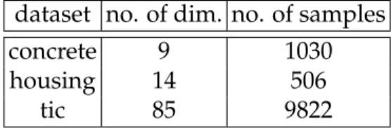
Three open benchmark datasets, “concrete,” “housing,” and “tic” from UCI (University of California Irvine) machine learning repository are used5(Asuncion & Newman, 2007). Table 2 shows properties of the datasets.

í10 í5 0 5 10 15 20 í10 í8 í6 í4 í2 0 2 4 í10 í5 0 5 10 15 20 í10 í8 í6 í4 í2 0 2 4 (a) Distribution (b) FKp (n=1000), Eemp =0.206,D =0 í10 í5 0 5 10 15 20 í10 í8 í6 í4 í2 0 2 4 í10 í5 0 5 10 15 20 í10 í8 í6 í4 í2 0 2 4 (c) SubKp (m =50), (d) RKp (n=50), Eemp =0.207,D=0.008 Eemp =0.232,D =0.157 í10 í5 0 5 10 15 20 í10 í8 í6 í4 í2 0 2 4 í10 í5 0 5 10 15 20 í10 í8 í6 í4 í2 0 2 4

(e) IKp (m =50), (f) Nys

Eemp =0.990,D=0.990 Eemp =0.383,D =0.192 í10 í5 0 5 10 15 20 í10 í8 í6 í4 í2 0 2 4 í10 í5 0 5 10 15 20 í10 í8 í6 í4 í2 0 2 4 (g) SpKp (σ=0.3,n =69.) (h)r=1 Eemp =0.357,D=0.843

Fig. 2. Contour curves of projection norms

Gaussian kernel k(x₁.x₂) = exp(−x₁₋x₂2/(2σ2)) whose σ2 is set to be the variance of for all elements of each dataset is used for the kernel function. The number of principal

dataset no. of dim. no. of samples

concrete 9 1030

housing 14 506

tic 85 9822

Table 2. Open dataset

components, r, is set to be the input dimension of each dataset. 90% of samples are used for training, and the remaining 10% of samples are used for validation. The division of the training and the validation sets is repeated 50 times randomly.

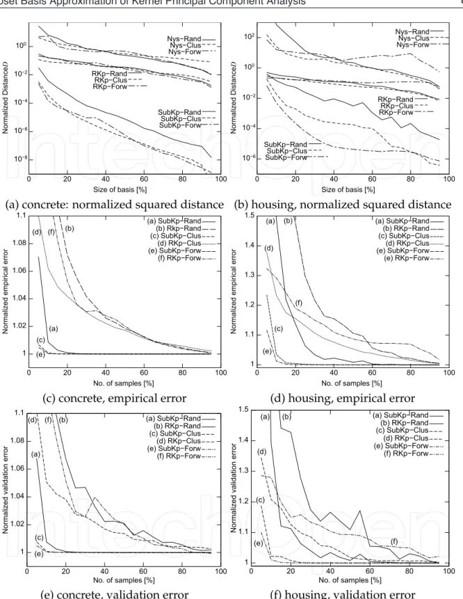
Figures 3-(a) and (b) show the averaged squared distance from KPCA using all samples. SubKPCA shows better performance than Reduced KPCA and the Nyström method, especially SubKPCA with a forward search performed the best of all. In both datasets, even if the number of basis is one of tenth that of all samples, the distance error of SubKPCA is less than 1%.

Figures 3-(c) and (d) show the average normalized empirical error, and Figures (e) and (f) show the averaged validation error. SubKPCA with K-means or forward search performed the best, and its performance did not change much with 20% more basis. The results for the Nyström method are outside of the range illustrated in the figures.

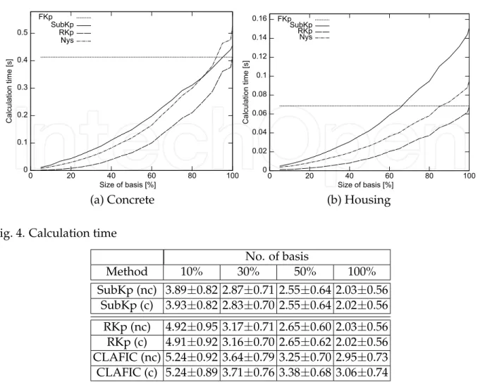
Figures 4-(a) and (b) show the calculation times for construction. The simulation was done on the system that has an Intel Core 2 Quad CPU 2.83GHz and an 8Gbyte RAM. The routines dsygvx and dsyevx in the Intel math kernel library (MKL) were respectively used for the generalized eigenvalue decomposition of SubKPCA and the eigenvalue decomposition of KPCA. The figures indicate that SubKPCA is faster than Full KPCA if the number of basis is less than 80%.

Figure 5 shows the relation between runtime [s] and squared distance from Full KPCA. In this figure, “kmeans” includes runtime for K-means clustering. The vertical dotted line stands for run-time of full KPCA. For (a) concrete and (b) housing, incomplete Cholesky decomposition is faster than our method. However, for a larger dataset, (c) tic, incomplete Cholesky decomposition is slower than our method. KHA-SMD Günter et al. (2007) is slower than full KPCA in these three methods.

6.4 Classification

PCA and KPCA are also used for classifier as subspace methods (Maeda & Murase, 1999; Oja, 1983; Tsuda, 1999). Subspace methods obtain projectors onto subspaces that correspond with classes. LetP_i be a projector onto the subspace of the classi. In the class feature information compression (CLAFIC) that is one of the subspace methods,P_iis a projector of PCA for each class. Then an input samplexis classified to a classkwhose squared distance is the largest, that is,

k=argmax

i=1,...,c

x₋P_ix2, (48)

where c is the number of classes. Binary classifiers such as SVM cannot be applied to multi-class problems directly, therefore, some extentions such as one-against-all strategy have to be used. However, subspace methods can be applied to many-class problems

10í8 10í6 10í4 10í2 100 0 20 40 60 80 100 N o rma lize d D ist a n ce D Size of basis [%] SubKpíRand RKpíRand NysíRand SubKpíClus RKpíClus NysíClus SubKpíForw RKpíForw NysíForw 10í6 10í4 10í2 100 102 0 20 40 60 80 100 N o rma lize d D ist a n ce D Size of basis [%] SubKpíRand RKpíRand NysíRand SubKpíClus RKpíClus NysíClus SubKpíForw RKpíForw NysíForw

(a) concrete: normalized squared distance (b) housing, normalized squared distance

1 1.02 1.04 1.06 1.08 1.1 0 20 40 60 80 100 N o rma lize d e mp iri ca l e rro r No. of samples [%]

(a) SubKpíRand

(a) (b) RkpíRand (b) (c) SubKpíClus (c) (d) RKpíClus (d)

(e) SubKpíForw

(e) (f) RKpíForw (f) 1 1.1 1.2 1.3 1.4 1.5 0 20 40 60 80 100 N o rma lize d e mp iri ca l e rro r No. of samples [%]

(a) SubKpíRand (a) (b) RKpíRand (b) (c) SubKpíClus (c) (d) RKpíClus

(d) _{(e) SubKpíForw}

(f)

(e) RKpíForw

(e)

(c) concrete, empirical error (d) housing, empirical error

1 1.02 1.04 1.06 1.08 1.1 0 20 40 60 80 100 N o rma lize d va lid a ti o n e rro r No. of samples [%]

(a) SubKpíRand

(a) (b) RKpíRand (b) (c) SubKpíClus (c) (d) RKpíClus (d)

(e) SubKpíForw

(e) (f) RKpíForw (f) 1 1.1 1.2 1.3 1.4 1.5 0 20 40 60 80 100 N o rma lize d va lid a ti o n e rro r No. of samples [%]

(a) SubKpíRand (a) (b) RKpíRand (b) (c) SubKpíClus (c) (d) RKpíClus

(d) (e) SubKpíForw

(e)

(f) RKpíForw

(f)

(e) concrete, validation error (f) housing, validation error

Fig. 3. Results for open datasets. Rand: random, Clus: Clustering (K-means), Forw: Forward search

easily. Furthermore, subspace methods are easily to be applied to multi-label problems or class-addition/reduction problems. CLAFIC is easily extended to KPCA (Maeda & Murase, 1999; Tsuda, 1999).

0 0.1 0.2 0.3 0.4 0.5 0 20 40 60 80 100 C a lcu la ti o n t ime [ s] Size of basis [%] FKp SubKp RKp Nys 0 0.02 0.04 0.06 0.08 0.1 0.12 0.14 0.16 0 20 40 60 80 100 C a lcu la ti o n t ime [ s] Size of basis [%] FKp SubKp RKp Nys

(a) Concrete (b) Housing

Fig. 4. Calculation time

No. of basis Method 10% 30% 50% 100% SubKp (nc) 3.89±0.82 2.87±0.71 2.55±0.64 2.03±0.56 SubKp (c) 3.93_±0.82 2.83_±0.70 2.55_±0.64 2.02_±0.56 RKp (nc) 4.92_±0.95 3.17_±0.71 2.65_±0.60 2.03_±0.56 RKp (c) 4.91±0.92 3.16±0.70 2.65±0.62 2.02±0.56 CLAFIC (nc) 5.24_±0.92 3.64_±0.79 3.25_±0.70 2.95_±0.73 CLAFIC (c) 5.24_±0.89 3.71_±0.76 3.38_±0.68 3.06_±0.74

Table 3. Minimum validation errors [%] and standard deviations I; random selection, nc: non-centered, c: centered

A handwritten digits database, USPS (U.S. postal service database), is used for the demonstration. The database has 7291 images for training, and 2001 images for testing. Each image is 16x16 pixel gray-scale, and has a label (0, . . . , 9).

10% of samples (729 samples) from training set are extracted for validation, and rest 90% (6562 samples) are used for training. This division is repeated 100 times, and obtained the optimal parameters from several picks, width of Gaussian kernel c _{∈ {}10−4.0, 10−3.8, . . . , 100.0_}, the number of principal componentsr_{∈ {}10, 20, . . . , 200_}.

Tables 3 and 4 respectively show the validation errors [%] and standard deviations over 100 validations when the samples of the basis are selected randomly and by k-means respectively. SubKPCA has lower error rate than reduced KPCA when the number of basis is small. Tables 5 and 6 show the test errors when the optimum parameters are given by the validation.

6.5 Denoising using a huge dataset

KPCA is also used for image denoising (Kim et al., 2005; Mika et al., 1999). This subsection demonstrate image denoising by KPCA using MNIST database. The database has 60000 images for training, and 10000 samples for testing. Each image is a 28x28 pixel gray-scale image of a handwritten digit. Each pixel value of the original image is scaled from 0 to 255.

10í10 10í8 10í6 10í4 10í2 100 10í3 ₁₀í2 ₁₀í1 ₁₀0 D ist a n ce f ro m KP C A Elapsed time [s] KHAíSMD ICD Kmeans SubKp Kmeans RKp Rand SubKp Rand RKp Rand SubKp+ICD FKp (a) Concrete 10í10 10í8 10í6 10í4 10í2 100 10í3 10í2 10í1 D ist a n ce f ro m KPC A Elapsed time [s] KHA_íSMD ICD Kmeans SubKp Kmeans RKp Rand SubKp Rand RKp Rand SubKp+ICD FKp (b) Housing 10í4 10í3 10í2 10í1 100 10í1 ₁₀0 ₁₀1 ₁₀2 ₁₀3 D ist a n ce f ro m KPC A Elapsed time [s] KHA_íSMD ICD Kmeans SubKp Kmeans RKp Rand SubKp Rand RKp Rand SubKp+ICD FKp (c) Tic

Fig. 5. Relation between runtime [s] and squared distance from Full KPCA No. of basis Method 10% 30% 50% 100% SubKp (nc) 2.69_±0.58 2.30_±0.61 2.18_±0.58 2.03_±0.56 SubKp (c) 2.68_±0.60 2.29_±0.61 2.15_±0.55 2.02_±0.56 RKp (nc) 2.75±0.61 2.35±0.60 2.22±0.57 2.03±0.56 RKp (c) 2.91_±0.63 2.40_±0.59 2.24_±0.58 2.02_±0.56 PCA (nc) 3.60±0.66 3.38±0.60 3.21±0.56 3.03±0.60

Table 4. Minimum validation errors [%] and standard deviations II; K-means, nc: non-centered, c: centered

Before the demonstration of image denoising, comparisons of computational complexities are presented since the database has rather large data. The Gaussian kernel functionk(x₁,x2) =

exp(₋10−5.1x1−x22)and the number of principal componentsr = 145 are used because

No. of basis Method 10% 30% 50% 100% SubKp (nc) 6.50±0.36 5.69±0.15 5.20±0.14 4.78±0.00 SubKp (c) 6.54_±0.36 5.52_±0.16 5.20_±0.14 4.83_±0.00 RKp (nc) 7.48_±0.44 5.71_±0.31 5.26_±0.20 4.78_±0.00 RKp (c) 7.50±0.43 5.76±0.31 5.28±0.20 4.83±0.00

Table 5. Test errors [%] and standard deviations; random selection, nc: non-centered, c: centered No. of basis Method 10% 30% 50% 100% SubKp (nc) 5.14±0.17 4.99±0.14 4.97±0.13 4.78±0.00 SubKp (c) 5.14_±0.18 4.99_±0.14 4.87_±0.14 4.83_±0.00 RKp (nc) 5.18_±0.21 5.01_±0.16 4.89_±0.15 4.78_±0.00 RKp (c) 5.36±0.24 5.07±0.17 4.93±0.15 4.83±0.00

Table 6. Test errors [%] and standard deviations; K-means, nc: non-centered, c: centered

4eí5 5eí5 6eí5 7eí5 8eí5 9eí5 1eí4 10í2 10í1 100 101 102 103 T ra in in g e rro r Elapsed time [s] ICD RKPCA SubKPCA

Fig. 6. Relation between training error and elapsed time in MNIST dataset

is used for basis of the SubKPCA. Figure 6 shows relation between run-time and training error. SubKPCA achieves lower training error Eemp = 4.57×10−5 in 28 seconds, whereas

Denoising is done by following procedures, 1. Rescale each pixel value from 0 to 1.

2. Obtain the subset using K-means clustering from 60000 training samples. 3. Obtain operators,

(a) Obtain centered SubKPCA using 60000 training samples and the subset. (b) Obtain centered KPCA using the subset.

4. Prepare noisy images using 10000 test samples; (a) Add Gaussian noise whose variance isσ2.

(b) Add salt-and-pepper noise with a probability of p (a pixel flips white (1) with probability p/2, and flips black (0) with probabilityp/2).

5. Obtain each transformed vector and pre-image using the method in (Mika et al., 1999). 6. Rescale each pixel value from 0 to 255, and truncate values if the values less than 0 or grater

than 255.

The evaluation criterion is the mean squared error EMSE= 1 10000 10000

∑

wheref_iis theith original test image, and ˆf is its denoising image. The optimal parameters, r: the number of principal components, and c: parameter of the Gaussian kernel, are chosen to show the best performance in several picks r _{∈ {}5, 10, 15, . . . ,m_} and c _∈ {10−6.0, 10−5.9, . . . , 10−2.0_}.

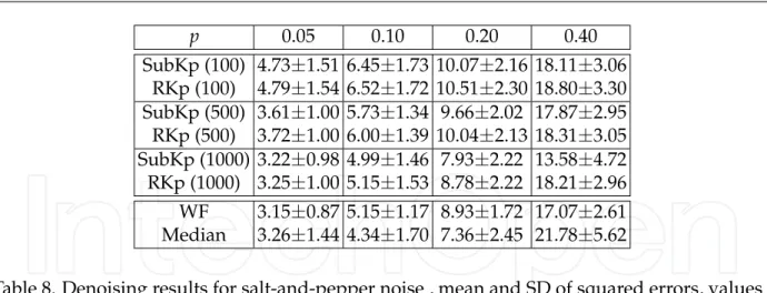
Tables 7 and 8 are denoising results. SubKPCA shows always lower errors than errors of Reduced KPCA. Figures 7 show the original images, noisy images, and de-noised images. Fields of experts (FoE) Roth & Black (2009) and block-matching and 3D filtering (BM3D) Dabov et al. (2007) are state-of-the-art denoising methods for natural images6. FoE and BM3D

σ 20 50 80 100 SubKp (100) 3.38_±1.37 4.64_±1.49 6.73_±1.70 8.33_±2.17 RKp (100) 3.48±1.42 4.71±1.51 6.80±1.74 8.55±2.11 SubKp (500) 0.99_±0.24 3.64_±0.82 6.22_±1.43 7.95_±1.91 RKp (500) 1.01_±0.27 3.73_±0.81 6.39_±1.51 8.14_±2.01 SubKp (1000) 0.93_±0.22 3.20_±0.83 5.11_±1.67 6.18_±2.02 RKp (1000) 0.94±0.20 3.27±0.87 5.49±1.60 7.18±1.88 WF 0.88_±0.24 3.14_±0.81 5.49_±1.43 7.01_±1.84 FoE 1.15_±2.08 8.48_±0.78 23.29_±1.90 36.53_±2.81 BM3D 1.07±1.80 7.17±1.09 17.39±2.96 25.49±4.17

Table 7. Denoising results for Gaussian noise , mean and SD of squared errors, values are divided by 105; the numbers in brackets denote the numbers of basis

6_{MATLAB codes were downloaded fromhttp://www.gris.}

tu-darmstadt.de/˜sroth/research/foe/downloads.html. and

p 0.05 0.10 0.20 0.40 SubKp (100) 4.73_±1.51 6.45_±1.73 10.07_±2.16 18.11_±3.06 RKp (100) 4.79_±1.54 6.52_±1.72 10.51_±2.30 18.80_±3.30 SubKp (500) 3.61±1.00 5.73±1.34 9.66±2.02 17.87±2.95 RKp (500) 3.72±1.00 6.00±1.39 10.04±2.13 18.31±3.05 SubKp (1000) 3.22_±0.98 4.99_±1.46 7.93_±2.22 13.58_±4.72 RKp (1000) 3.25_±1.00 5.15_±1.53 8.78_±2.22 18.21_±2.96 WF 3.15_±0.87 5.15_±1.17 8.93_±1.72 17.07_±2.61 Median 3.26_±1.44 4.34_±1.70 7.36_±2.45 21.78_±5.62

Table 8. Denoising results for salt-and-pepper noise , mean and SD of squared errors, values are divided by 105; the numbers in brackets denote the numbers of basis

are assumed that the noise is Gaussian whose mean is zero and variance is known. Thus these two methods are compared only in Gaussian noise case. Since the datasets is not natural images, these methods are not better than SubKPCA. “WF” and “Median” denote Wiener filter and median filter respectively. When noise is relatively small, (σ = 20 _∼ 50 in Gaussian or p=0.05_∼0.10), these classical methods show better performance. On the other hand, when noise is large, our method shows better performance. Note that Wiener filter is known to be the optimal filter in terms of the mean squared error among linear operators. From different point of view, Wiener filter is optimal among all linear and non-linear operators if both signal and noise are Gaussian. However, KPCA is non-linear because of non-linear mappingΦ_{, and}

pixel values of images and salt-and-pepper noise are not Gaussian in this case.

(a) Gaussian noise (b) Salt-and-pepper-noise Fig. 7. Results of denoising (first 100 samples), top-left: original image, top-right: noisy image (Gaussian,σ=50), bottom-left: image de-noised by SubKPCA, bottom-right: image de-noised by KPCA.

7. Conclusion

Theories, properties, and numerical examples of SubKPCA have been presented in this chapter. SubKPCA has a simple solution form Eq. (22) and no constraint for its kernel functions. Therefore, SubKPCA can be applied to any applications of KPCA. Furthermore, it should be emphasized that SubKPCA is always better than reduced KPCA in the sense of the empirical errors if the subset is the same.

8. References

Asuncion, A. & Newman, D. (2007). UCI machine learning repository. URL:http://www.ics.uci.edu/_∼mlearn/MLRepository.html

Bach, F. R. & Jordan, M. I. (2002). Kernel independent component analysis,Journal of Machine Learning Research3: 1–48.

Dabov, K., Foi, A., Katkovnik, V. & Egiazarian, K. (2007). Image denoising by sparse 3D transform-domain collaborative filtering, IEEE Trans. on Image Processing 16(8): 2080–2095.

Demmel, J. (1997). Applied Numerical Linear Algebra, Society for Industrial Mathematics. Ding, M., Tian, Z. & Xu, H. (2010). Adaptive kernel principal component analysis, Signal

Processing90(5): 1542–1553.

Girolami, M. (2002). Mercer kernel-based clustering in feature space, IEEE Trans. on Neural Networks13(3): 780–784.

Gorban, A., Kégl, B., Wunsch, D. & (Eds.), A. Z. (2008).Principal Manifolds for Data Visualisation and Dimension Reduction, LNCSE 58, Springer.

Günter, S., Schraudolph, N. N. & Vishwanathan, S. V. N. (2007). Fast iterative kernel principal component analysis,Journal of Machine Learning Research8: 1893–1918.

Harville, D. A. (1997). Matrix Algebra From a Statistician’s Perspective, Springer-Verlag.

Hastie, T. & Stuetzle, W. (1989). Principal curves,Journal of the American Statistical Association Vol. 84(No. 406): 502–516.

Israel, A. B. & Greville, T. N. E. (1973). Generalized inverses, Theorey and applications, Springer. Kim, K., Franz, M. O. & Schölkopf, B. (2005). Iterative kernel principal component

analysis for image modeling, IEEE Trans. Pattern Analysis and Machine Intelligence 27(9): 1351–1366.

Lehoucq, R. B., Sorensen, D. C. & Yang, C. (1998). ARPACK Users’ Guide: Solution of Large-Scale Eigenvalue Problems with Implicitly Restarted Arnoldi Methods, Software, Environments, and Tools 6, SIAM.

Maeda, E. & Murase, H. (1999). Multi-category classification by kernel based nonlinear subspace method, IEEE International Conference On Acoustics, speech, and signal processing (ICASSP), Vol. 2, IEEE press., pp. 1025–1028.

Mika, S., Schölkopf, B. & Smola, A. (1999). Kernel PCA and de-noising in feature space, Advances in Neural Information Processing Systems (NIPS)11: 536–542.

Oja, E. (1983). Subspace Methods of Pattern Recognition, Wiley, New-York.

Platt, J. C. (1999). Fast training of support vector machines using sequential minimal optimization, in B. Scholkopf, C. Burges & A. J. Smola (eds), Advances in Kernel Methods - Support Vector Learning, MIT press, pp. 185–208.

Roth, S. & Black, M. J. (2009). Fields of experts, International Journal of Computer Vision 82(2): 205–229.

Roweis, S. T. & Saul, L. K. (2000). Nonlinear dimensionality reduction by locally linear embedding,Science290: 2323–2326.

Schölkopf, B., Mika, S., Burges, C., Knirsch, P., Müller, K.-R., Rätsch, G. & Smola, A. (1999). Input space vs. feature space in kernel-based methods,IEEE Trans. on Neural Networks 10(5): 1000–1017.

Schölkopf, B., Smola, A. & Müller, K.-R. (1998). Nonlinear component analysis as a kernel eigenvalue problem,Neural Computation10(5): 1299–1319.

Smola, A. J., Mgngasarian, O. L. & Schölkopf, B. (1999). Sparse kernel feature analysis, Technical report 99-04, University of Wisconsin.

Tenenbaum, J. B., de Silva, V. & Langford, J. C. (2000). A global geometric framework for nonlinear dimensionality reduction,Science290: 2319–2323.

Tipping, M. E. (2001). Sparse kernel principal component analysis, Advances in Neural Information Processing Systems (NIPS)13: 633–639.

Tsuda, K. (1999). Subspace classifier in the Hilbert space, Pattern Recognition Letters 20: 513–519.

Vapnik, V. (1998). Statistical Learning Theory, Wiley, New-York.

Washizawa, Y. (2009). Subset kernel principal component analysis,Proceedings of 2009 IEEE International Workshop on Machine Learning for Signal Processing, IEEE, pp. 1–6.

Williams, C. K. I. & Seeger, M. (2001). Using the Nyström method to speed up kernel machines, Advances in Neural Information Processing Systems (NIPS)13: 682–688.

Xu, Y., Zhang, D., Song, F., Yang, J., Jing, Z. & Li, M. (2007). A method for speeding up feature extraction based on KPCA,Neurocomputingpp. 1056–1061.

ISBN 978-953-51-0195-6 Hard cover, 300 pages

Publisher InTech

Published online 02, March, 2012

Published in print edition March, 2012

InTech Europe

University Campus STeP Ri Slavka Krautzeka 83/A 51000 Rijeka, Croatia Phone: +385 (51) 770 447 Fax: +385 (51) 686 166 www.intechopen.com

InTech China

Unit 405, Office Block, Hotel Equatorial Shanghai No.65, Yan An Road (West), Shanghai, 200040, China Phone: +86-21-62489820

Fax: +86-21-62489821

This book is aimed at raising awareness of researchers, scientists and engineers on the benefits of Principal Component Analysis (PCA) in data analysis. In this book, the reader will find the applications of PCA in fields such as image processing, biometric, face recognition and speech processing. It also includes the core concepts and the state-of-the-art methods in data analysis and feature extraction.

How to reference

In order to correctly reference this scholarly work, feel free to copy and paste the following:

Yoshikazu Washizawa (2012). Subset Basis Approximation of Kernel Principal Component Analysis, Principal Component Analysis, Dr. Parinya Sanguansat (Ed.), ISBN: 978-953-51-0195-6, InTech, Available from: http://www.intechopen.com/books/principal-component-analysis/subset-basis-approximation-of-kernel-principal-component-analysis

distributed under the terms of the

Creative Commons Attribution 3.0

License

, which permits unrestricted use, distribution, and reproduction in