Doctoral Dissertations Student Theses and Dissertations
Spring 2020
Strengthening QC relaxations of optimal power flow problems by
Strengthening QC relaxations of optimal power flow problems by
exploiting various coordinate changes
exploiting various coordinate changes
Mohammad Rasoul NarimaniFollow this and additional works at: https://scholarsmine.mst.edu/doctoral_dissertations
Part of the Electrical and Computer Engineering Commons Department: Electrical and Computer Engineering
Department: Electrical and Computer Engineering
Recommended Citation Recommended Citation
Narimani, Mohammad Rasoul, "Strengthening QC relaxations of optimal power flow problems by exploiting various coordinate changes" (2020). Doctoral Dissertations. 2873.
https://scholarsmine.mst.edu/doctoral_dissertations/2873
This thesis is brought to you by Scholars' Mine, a service of the Missouri S&T Library and Learning Resources. This work is protected by U. S. Copyright Law. Unauthorized use including reproduction for redistribution requires the permission of the copyright holder. For more information, please contact [email protected].
BY EXPLOITING VARIOUS COORDINATE CHANGES
by
MOHAMMAD RASOUL NARIMANI
A DISSERTATION
Presented to the Graduate Faculty of the
MISSOURI UNIVERSITY OF SCIENCE AND TECHNOLOGY
In Partial Fulfillment of the Requirements for the Degree
DOCTOR OF PHILOSOPHY
in
ELECTRICAL ENGINEERING
2020
Approved by
Mariesa L. Crow, Advisor Daniel K. Molzahn
Pourya Shamsi Mehdi Ferdowsi Jonothan W. Kimball
MOHAMMAD RASOUL NARIMANI All Rights Reserved
PUBLICATION DISSERTATION OPTION
This dissertation consists of the following five articles which have been submitted for publication, or will be submitted for publication as follows:
Paper I: Empirical investigation of non-convexities in optimal power flow problems. Published in American Control Conference, pp. 27-54.
Paper II: Improving QC Relaxations of OPF Problems Via Voltage Magnitude Dif-ference Constraints and Envelopes for Trilinear Monomials. Published in Power Systems Computation Conference, pp. 55-78.
Paper III: Comparison of Various Trilinear Monomial Envelopes for Convex Relax-ations of Optimal Power Flow Problems, pp.79-94.
Paper IV: Tightening QC Relaxations of AC Optimal Power Flow Problems Via Complex Per Unit Normalization. Submitted to IEEE Transaction on Power System, pp. 95-131.
Paper V: Tightening QC Relaxations of OPF Problems by Independently Rotating the Trigonometric Terms. is intended to submit to IEEE Transaction on Power System, pp. 132-163.
ABSTRACT
Motivated by the potential for improvements in electric power system economics, this dissertation studies the AC optimal power flow (AC OPF) problem. An AC OPF problem optimizes a specified objective function subject to constraints imposed by both the non-linear power flow equations and engineering limits. The difficulty of an AC OPF problem is strongly connected to its feasible space’s characteristics. This dissertation first investigates causes of nonconvexities in AC OPF problems. Understanding typical causes of nonconvexities is helpful for improving AC OPF solution methodologies.
This dissertation next focuses on solution methods for AC OPF problems that are based onconvex relaxations. The quadratic convex (QC) relaxation is one promising ap-proach that constructs convex envelopes around the trigonometric and product terms in the polar representation of the power flow equations. This dissertation proposes several im-provements to strengthen QC relaxations of OPF problems. The first group of imim-provements provides tighter envelopes for the trigonometric functions and product terms in the power flow equations. Methods for obtaining tighter envelopes includes implementing Meyer and Floudas envelopes that yield the convex hull of trilinear monomials. Furthermore, by leveraging a representation of line admittances in polar form, this dissertation proposes tighter envelopes for the trigonometric terms. Another proposed improvement exploits the ability to rotate the base power used in the per unit normalization in order to facilitate the application of tighter trigonometric envelopes.
The second group of improvements propose additional constraints based on new variables that represent voltage magnitude differences between connected buses. Using “bound tightening” techniques, the bounds on the voltage magnitude differencevariables can be significantly tighter than the bounds on the voltage magnitudes themselves, so constraints based on voltage magnitude differences can improve the QC relaxation.
ACKNOWLEDGMENTS
Firstly, I would like to express my sincere gratitude to my advisor Prof. Mariesa Crow for the continuous support of my Ph.D study and related research, for her patience, motivation, and immense knowledge. Her guidance helped me in all the time of research and writing of this dissertation. I would also like to express my deepest gratitude to my co-advisor, Dr. Daniel Molzahn. The depth and breadth of his knowledge showed me the importance of drawing on ideas from a variety of areas to solve practical and challenging problems. It has been a great experience to work under his guidance and I attribute the level of my PhD degree to his encouragement and effort. I will forever remain indebted for his tutelage. I am also very grateful for the assistance and advice provided by my doctoral committee. Dr. Mehdi Ferdowsi guidance in numerous situations and his support through GAAN fellowship have been invaluable. Dr. Pourya Shamsi inspired me to pursue a research career in electric power. I also greatly benefited from Dr. Kimball vast knowledge of power electronic and electric machines. Drawing on this knowledge would be essential to my career. I would also like to thank Dr. long for serving on my committee.
I would like to express my deepest gratitude for the support and love of my family. I can never thank my parents, enough for their encouragement and love. Finally, I greatly appreciate the companionship and patience of my wife, Fatemeh Narimani. Her support throughout my graduate studies was essential to my success. It would never have done without her support. I can never thank my wife enough for her encouragement and love. I will forever remain indebted for her support. I gratefully acknowledge the support of the research assistantships funded by grants from the Department of Energy, and the GAAN fellowship funded from the Department of Education.
TABLE OF CONTENTS
Page
PUBLICATION DISSERTATION OPTION . . . iii
ABSTRACT . . . iv
ACKNOWLEDGMENTS . . . v
LIST OF ILLUSTRATIONS . . . xi
LIST OF TABLES . . . xiii
SECTION 1. INTRODUCTION . . . 1
1.1. MOTIVATION . . . 1
1.2. THE POWER FLOW EQUATIONS . . . 3
1.3. LITERATURE REVIEW . . . 7
1.3.1. Semidefinite Programming Relaxations of the Power Flow Equations 7 1.3.1.1. The Shor relaxation . . . 7
1.3.1.2. Moment/sum-of-square relaxation hierarchies . . . 9
1.3.2. Second-Order Cone Programming Relaxation of the Power Flow Equations . . . 9
1.3.2.1. Bus injection model relaxations . . . 10
1.3.2.2. Branch flow model relaxations. . . 12
1.3.3. Linear Relaxation of the Power Flow Equations . . . 13
1.3.3.1. The network flow relaxation . . . 13
1.3.3.3. The Taylor-Hoover relaxation . . . 14
1.3.3.4. McCormick relaxations . . . 15
1.3.3.5. Bienstock-Munoz LP relaxations . . . 16
1.3.3.6. Mixed-integer linear programming relaxations . . . 17
1.4. THE OPTIMAL POWER FLOW PROBLEM. . . 18
1.5. QC RELAXATION . . . 20
1.6. QC RELAXATION OF THE POWER FLOW EQUATIONS . . . 20
1.7. CONTRIBUTIONS . . . 24
1.8. TERMINOLOGIES . . . 25
PAPER I. EMPIRICAL INVESTIGATION OF NON-CONVEXITIES IN OPTIMAL POWER FLOW PROBLEMS . . . 27
ABSTRACT . . . 27
1. INTRODUCTION . . . 28
2. OVERVIEW OF THE OPF PROBLEM . . . 31
2.1. TOOLS FOR STUDYING OPF FEASIBLE SPACES . . . 33
2.2. COMPUTING THE FEASIBLE SPACES OF SMALL OPF PROB-LEMS . . . 34
2.3. COMPUTING MULTIPLE LOCAL OPTIMA . . . 35
3. INVESTIGATING THE CAUSES OF OPF NON-CONVEXITIES VIA A NUMERICAL EXPERIMENT . . . 35
3.1. RANDOMLY GENERATING AND SCREENING SMALL TEST CASES . . . 36
3.2. ILLUSTRATIVE EXAMPLES OF OPF FEASIBLE SPACES . . . 38
4. CHALLENGING OPF PROBLEMS DERIVED BY MODIFYING IEEE TEST CASES . . . 44
5. CONCLUSION . . . 46
II. IMPROVING QC RELAXATIONS OF OPF PROBLEMS VIA VOLTAGE MAGNITUDE DIFFERENCE CONSTRAINTS AND ENVELOPES FOR
TRI-LINEAR MONOMIALS . . . 52
ABSTRACT . . . 52
1. INTRODUCTION . . . 53
2. OVERVIEW OF OPTIMAL POWER FLOW PROBLEM . . . 54
3. REVIEW OF THE QC RELAXATION . . . 56
3.1. FORMULATION OF THE QC RELAXATION . . . 56
3.2. BOUND TIGHTENING AND OTHER IMPROVEMENTS . . . 59
4. VOLTAGE MAGNITUDE DIFFERENCE CONSTRAINTS . . . 60
5. TRILINEAR ENVELOPES . . . 63
6. NUMERICAL RESULTS . . . 66
7. CONCLUSION . . . 71
BIBLIOGRAPHY . . . 71
III. COMPARISON OF VARIOUS TRILINEAR MONOMIAL ENVELOPES FOR CONVEX RELAXATIONS OF OPTIMAL POWER FLOW PROBLEMS . . . 74
ABSTRACT . . . 74
1. INTRODUCTION . . . 75
2. OPTIMAL POWER FLOW OVERVIEW . . . 76
3. THE QC RELAXATION . . . 78
3.1. SQUARED VOLTAGE MAGNITUDE AND TRIGONOMETRIC ENVELOPES . . . 78
3.2. RECURSIVE MCCORMICK ENVELOPES FOR TRILINEAR MONOMIALS. . . 79
3.3. MEYER AND FLOUDAS ENVELOPES FOR TRILINEAR MONO-MIALS . . . 80
3.4. EXTREME POINT ENVELOPES FOR TRILINEAR MONOMIAS 80 3.5. FORMULATION OF THE QC RELAXATION . . . 82
5. CONCLUSIONS . . . 87
BIBLIOGRAPHY . . . 87
IV. TIGHTENING QC RELAXATIONS OF AC OPTIMAL POWER FLOW PROB-LEMS VIA COMPLEX PER UNIT NORMALIZATION . . . 91
ABSTRACT . . . 91
1. INTRODUCTION . . . 92
2. OVERVIEW OF THE OPTIMAL POWER FLOW PROBLEM . . . 94
3. THE QC RELAXATION OF THE OPF PROBLEM . . . 95
4. COORDINATE TRANSFORMATIONS . . . 98
4.1. POWER FLOW EQUATIONS WITH ADMITTANCE IN POLAR FORM . . . 98
4.2. ROTATED POWER FLOW FORMULATION . . . 99
4.3. ROTATED OPF PROBLEM . . . 101
5. ROTATED QC RELAXATION . . . 102
5.1. CONVEX ENVELOPES FOR THE TRIGONOMETRIC TERMS . . 103
5.2. ENVELOPES FOR TRILINEAR TERMS . . . 110
5.3. QC RELAXATION OF THE ROTATED OPF PROBLEM . . . 115
5.4. TIGHTENED QC RELAXATION OF THE ROTATED OPF PROB-LEM . . . 117
5.5. AN EMPIRICAL ANALYSIS FOR DETERMINING THE RO-TATIONψ. . . 118
6. MORE GENERAL LINE MODELS. . . 119
7. NUMERICAL RESULTS . . . 121
8. CONCLUSION . . . 124
BIBLIOGRAPHY . . . 124
V. TIGHTENING QC RELAXATIONS OF OPF PROBLEMS BY INDEPEN-DENTLY ROTATING THE TRIGONOMETRIC TERMS . . . 127
1. INTRODUCTION . . . 128
2. OVERVIEW OF OPTIMAL POWER FLOW PROBLEM . . . 130
3. OVERVIEW OF QC RELAXATION . . . 131
4. MODIFIED POWER FLOW EQUATIONS . . . 135
4.1. POWER FLOW EQUATIONS WITH ADMITTANCE IN POLAR FORM . . . 136
4.2. DIFFERENT REPRESENTATION OF POWER FLOW EQUA-TIONS . . . 137
4.3. THE OPF PROBLEM WITH MODIFIED POWER FLOW EQUA-TIONS . . . 138
5. QC RELAXATION OF THE PROPOSED OPF PROBLEM. . . 140
5.1. CONVEX ENVELOPES FOR THE TRIGONOMETRIC TERMS . . 140
5.2. ENVELOPES FOR TRILINEAR TERMS . . . 146
5.3. QC RELAXATION OF THE OPF PROBLEM WIHT MODIFIED DEFINITION OF THE POWER FLOW EQUATIONS . . . 148
5.4. TIGHTENED QC RELAXATION OF THE ROTATED OPF PROB-LEM . . . 149
5.5. AN APPROACH FOR DETERMINING THE SHIFTING VARI-ABLESψlmp1qANDψlmp2q . . . 150 BIBLIOGRAPHY . . . 154 SECTION 2. CONCLUSION . . . 157 BIBLIOGRAPHY . . . 158 VITA . . . 163
LIST OF ILLUSTRATIONS
Figure Page
1.1. Explanation of the variables in the DistFlow equations for linepi,kq PL [7]. . . . 12
1.2. Proven dominance relationships among relaxations. . . 18 1.3. Global and local optimum illustration. . . 25 1.4. Illustrating of tight and loos relaxations for a nonconvex function. . . 26 PAPER I
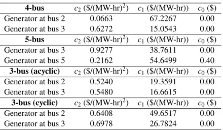
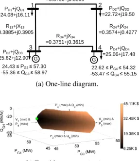
1. One-line diagram and feasible space projection for a “typical” randomly
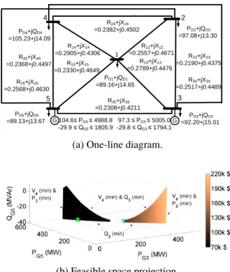
gen-erated four-bus test case. . . 41 2. One-line diagram and feasible space projection for a randomly generated
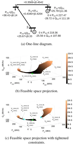
five-bus test case. . . 42 3. One-line diagram and feasible space projection for a randomly generated
acyclic three-bus test case. . . 43 4. Illustration of the voltage magnitude limits (1d). . . 44 5. One-line diagram and feasible space projection for a randomly generated cyclic
three-bus test case. . . 45 PAPER II
1. A projection of the feasible space for the “case6_c” [22] test system. . . 61 PAPER III
1. Run time comparisons of various formulations using three solvers. . . 86 PAPER IV
1. The left figures show visualizations of the function cospθlm´δlmq(black curve) and the line connecting the endpoints of this function atθlmminandθmaxlm (dashed red line) for different values ofδlm,θlmmin, andθlmmax. The right figures show the
corresponding functionFpθlmq. . . 107 2. Comparison of envelopes for the trigonometric terms in (1) and (15). . . 108 3. Comparison of envelopes for the sine and cosine functions for different values
ofψ. . . 111 SECTION
4. A projection of the four-dimensional polytope associated with the trilinear products between voltage magnitudes and trigonometric functions, in terms of the sending end variables ˜Slmpsq and ˜Clmpsq representing cospθlm´δlm ´ψqand
sinpθlm´δlm´ψq. . . 112 5. A projection of the four-dimensional polytope associated with the trilinear
products between the voltage magnitudes and the trigonometric functions, expressed in terms of the sending end variables ˜Slmpsq and ˜Clmpsq representing
cospθlm´δlm´ψqand sinpθlm´δlm´ψq. . . 113 6. Normalized optimality gap as a function ofψfor PGLib-OPF cases. . . 118 7. Comparison of optimality gap differences with respect to the original QC
relaxation (7) for different QC relaxation variants. . . 123 PAPER V
1. Comparison of envelopes for the trigonometric terms in (1) and (15). . . 144 2. Comparison of envelopes for the sine and cosine functions for different values
ofψlmp1q andψlmp2q. . . 145 3. A projection of the four-dimensional polytope associated with the trilinear
products between voltage magnitudes and trigonometric functions, in terms of the sending end variables ˜Slmpsq and ˜Clmpsqrepresenting cospθlm´δlm´ψ
p1q
lmq and sinpθlm´δlm´ψ
p2q
lmq. . . 147
4. Thea area between upper and lower portion envelopes of the sine function for
´30˝ ďθlm ď30˝, δlm “ ´53˝ andψlm,2 “24˝ (purple) andψlm,2 “ ´37˝
LIST OF TABLES
Table Page
PAPER I
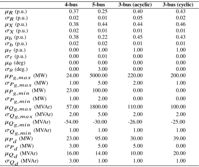
1. Means and standard deviations for parameter values in the randomly
con-structed test cases. . . 37
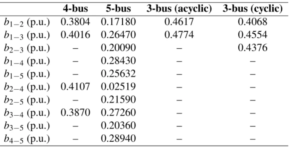
2. Line shunt values in randomly constructed test cases.. . . 39
3. Transformer details for the Five-bus test case. . . 40
4. Generation cost coefficients. . . 40
5. Voltage limits. . . 40
6. Descriptions of modifications to the IEEE test systems. . . 46
7. Objective values for the modified IEEE test cases. . . 46
PAPER II 1. Results from applying the QC relaxation with various improvements to selected test cases . . . 70
PAPER III 1. Variables and constraints per trilinear monomial envelope. . . 85
2. QC relaxation gaps using recursive McCormick (RMC) vs. convex-hull en-velopes (MF, EP). . . 86
PAPER IV 1. Line segment intersections corresponding to Figure 5 . . . 113
2. Coordinates of the line segment intersections in Table 1. . . 114
3. Results from applying the QC and RQC relaxations with various options to selected PGLib test cases.. . . 122
1. INTRODUCTION
1.1. MOTIVATION
The AC Optimal Power Flow (ACOPF) is at the heart of many problems in power system area. Independent System Operators (ISO) solve the AC OPF problem for various time slots, every year for system planning, everyday for day-ahead markets, every hour, and every five minutes for system operation [1]. The OPF is a fundamental optimization problem in power system that seeks decision variables to yield an optimal operating point in terms of a specific objective and subject to network equality constraints and engineering limits. Various objectives have been considered for solving OPF problems ranging from electricity generation cost, emission, power losses, reliability, etc. Economic operation of electric power systems is a major concern of power system engineers. With the large size of the power system industry in the United States even a slight improvement in electricity generation cost can save million of dollars annually. As one measure of industry size, electric industry revenues in the United States were $369 billion in 2010 [2], so, improvements in power system economics have the potential for significant impacts. This dissertation discusses research into the “optimal power flow” problem of minimizing generation cost while satisfying physical network constraints and engineering limits. Physical network constraints represent power flow equations that relates voltage phasors and power flow in lines. Engineering limits present practical restrictions of power systems such as voltage magnitudes, active and reactive generation, and line flow limits.
A wide range of engineering limits are involved in a typical OPF problem ranging from active and reactive power generation, bus voltage magnitudes, transmission line and transformer flows, and possibly network stability constraints. Like many optimization problems in power systems, power flow equations play a crucial role in the OPF problem relating voltage at buses to active and reactive power injections to buses. Nonconvexity in typical OPF formulations enters largely through the nonlinear power flow equations representing physical constraints on the electric grid. Using the nonlinear AC power flow model to accurately represent the power flow physics results in the AC OPF problem, which is non-convex, may have multiple local optima [1], and is generally NP-Hard [2], [3]. A wide variety of algorithms have been applied in order to find locally optimal solutions [4], [5]. The power flow equations are typically solved using iterative numerical techniques for systems of non-linear equations, such as the Newton-Raphson and Gauss-Seidel methods [6].
Many recent research efforts have developed convex relaxations of OPF problems to obtain bounds on the optimal objective values, certify infeasibility, and, in some cases, achieve globally optimal solutions. Solutions from a relaxation are also useful for initializing certain local solution techniques [7]. Convex relaxations are under active development with ongoing efforts aiming to improve the relaxations’ computational tractability and tightness. Recent work is surveyed in [7]. The quadratic convex (QC) relaxation [5] is one promising approach that uses convex envelopes around the trigonometric functions, squared terms, and bilinear products in the polar form of the power flow equations.
Using the QC relaxation of the optimal power flow problem, this dissertation details enhancements that enable economic operation of electric power systems. The power flow equations model the physical network constraints inherent to the optimal power flow prob-lem, which is used to minimize system operating costs. This dissertation investigates a QC relaxation relaxation of the optimal power flow problem and provides modeling necessary for application to electric power systems. Before delving into these contributions, this
in-troduction first provides a background on the power flow equations. Next a literature review on different convex relaxations of power flow equations is presented. Then the optimal power flow problem, and QC relaxation of OPF problem is explained.
1.2. THE POWER FLOW EQUATIONS
The goal of a power-flow study is to obtain voltages angle and magnitude informa-tion for each bus in a power system for specified load and generator real power and voltage conditions. All active and reactive power flow on each branch as well as generator reactive power output can be analytically determined by voltage angle and magnitudes. The underly-ing voltage-to-current relationships of the network are linear, but the nature of equipment in a power system is such that injected/demanded complex power at a bus is typically specified, rather than current. The relation of interest is between the active and reactive power injected at each bus and the complex voltages at each bus, and hence the associated equations are non-linear. Due to the nonlinear nature of this power flow equations, numerical methods are employed to obtain a solution that is within an acceptable tolerance. Using polar repre-sentation for complex voltages and rectangular “active/reactive” reprerepre-sentation of complex power, the power balance equations at busiare given by
Pi “Vi n ÿ
k“1
VkpGikcospδi´δkq `Biksinpδi´δkqq (1.1a)
Qi“Vi n ÿ
k“1
VkpGiksinpδi´δkq ´ Bikcospδi´δkqq (1.1b)
wherePiandQiare the active and reactive power injections, respectively, at busi,Viandδi are the voltage magnitude and phase angle, respectively, at busi,Y “G`j Bis the network admittance matrix [8], andnis the number of buses in the system.
The first step in solving the power flow problem is defining the known and unknown variables in the system. The known and unknown variables are dependent on the type of bus. A bus without any generators connected to it is called a Load Bus or PQ bus. PQ buses treatPiandQias specified quantities, and enforce the active power (1.1a) and reactive power (1.1b) equations at that bus. With one exception, a bus with at least one generator connected to it is called a generator bus or PV bus. The exception is one arbitrarily-selected bus that has a generator. This bus is referred to as the slack bus. PV buses, which typically correspond to generators, specify a known voltage magnitudeViand active power injection
Pi, and enforce only the active power equation (1.1a). The associated reactive powerQimay
be computed as an “output quantity,” via (1.1b). Finally, a single slack bus, with specified
Vi andδi (typically chosen to be 00) is selected. The active power Pi and reactive powerQi at the slack bus are determined from (1.1a) and (1.1b), respectively.
The line flows can be equivalently modeled using a polar representation of the line’s mutual admittance,Yikejδik, where Yik “
b
G2
ik `Bik2 and δik “ arctanpBik{Gikq are the magnitude and angle of the mutual admittance for linepi,kq P L, respectively. Using polar
admittance coordinates, the complex power flows into each terminal of the linepi,kq P L,
are: Pi “Vi n ÿ k“1 VkpYikcospδi´δk ´θikqq (1.2a) Qi “Vi n ÿ k“1 VkpYiksinpδi´δk´θikqq (1.2b)
The non-linear power flow equations require iterative numerical solution techniques, such as Gauss-Seidel or, most commonly, Newton-Raphson [8]. The Newton-Raphson method begins with initial guesses of all unknown variables. Next, a Taylor Series is written, with the higher order terms neglected, for each of the power balance equations (1.1a) and (1.1b).
The result is a linear system of equations that can be expressed as: » — – ∆θ ∆|V| fi ffi fl“ ´J ´1 » — – ∆P ∆Q fi ffi fl. (1.3)
∆Pand∆Qare the mismatch equations that can be expresed as follow:
∆Pi “ ´Pi`Vi n ÿ
k“1
VkpGikcospδi´δkq `Biksinpδi´δkqq (1.4a)
∆Qi “ ´Qi`Vi n ÿ
k“1
VkpGiksinpδi´δkq ´Bikcospδi´δkqq (1.4b)
J is the Jacobian matrix which consists of different partial derivatives of injected active and reactive power to each bus with respect to voltage magnitude and angle. The Jacobian matrix can be expressed as follow:
J “ » — – B∆P B∆θ B∆P B∆|V| B∆Q B∆θ B∆Q B∆|V| fi ffi fl. (1.5)
The voltage magnitude and angles can be computed iteratively using the linearized system of equations in (1.3) and an initial guess of the solution voltage magnitudes and angles as follow:
θm`1“θm`∆θ
(1.6) |V|m`1“ |V|m`∆|V| (1.7)
The iterative solving process continues until a stopping condition is met. A common stopping condition is to terminate if the norm of the mismatch equations is below a specified tolerance.
Note that the Newton-Raphson’s convergence performances strongly depends on the initial guess of the solution voltage magnitudes and angles. Newton methods are only locally convergent; there is no guarantee to converge to a particular solution from an arbitrary initial guess [6]. A initial guess consisting of a “flat start” voltage profile with uniform voltage magnitudes and zero phase angles can often be used to find a solution for “typical” parameters. However, it is important to recognize that as parameters move outside of routine operating ranges the behavior of the power flow equations can be highly complex, resulting in convergence failure for these solution techniques.
The properties of the Newton-Raphson iteration guarantee (under suitable differ-entiability assumptions) convergence to a solution for an initial condition selected in a sufficiently small neighborhood around that solution [9]. The existence of a power flow solution is necessary for power system stability analysis and plays a crucial role in power system reliability. However, selecting an arbitrary initial guess for power flow equation might give rise to divergence issues. The important point here is that the user cannot distin-guish the “no feasible solution” property for power flow equations and “bad initial guess” when they encounter divergence issues.
Power flow equations may have a very large number of solutions; for example, the work of [10] establishes cases for which the number of solutions grows faster than polynomial with respect to network size. Note that power systems typically operate at a high-voltage, stable solution. Thus, other power flow solutions, particularly those exhibiting low-voltage magnitude, are important to power system stability assessment and bifurcation analysis [11]- [15].
Convergence of local solution methods such as Newton Raphson method strongly depends on the selected initialization. Thus, initializing a local algorithm with various power flow solutions corresponding to random operating points is one approach for computing multiple local optima.
1.3. LITERATURE REVIEW
This section overviews convex relaxations of the power flow equations. Different variations of relevant power flow relaxation including Semi-Definite Programming, Second-Order Cone Programming, and Linear relaxation of power flow equation are overviewed in this section.
1.3.1. Semidefinite Programming Relaxations of the Power Flow Equations.
Expressing voltage in rectangular coordinate turns the power flow equations into a quadratic polynomials in the voltage components Vd and Vq. Having power flow equations as a quadratic polynomials facilitates the application of polynomial optimization theory, includ-ing the Shore relaxation and hierarchies of moment/sum-of-squares relaxations which are explained in the following subsections.
1.3.1.1. The Shor relaxation. The shore relaxation is a SDP relaxation of
non-convex quadratically constrained quadratic programs (QCQPs) which was first introduced in 1987 [16]. The first application of the Shor relaxation on power system problems was the relaxation of the optimal power flow (OPF) problem [17]. The SDP relaxation of OPF problems became an active avenue of research after showing that the SDP relaxation can solve the OPF problem globally for many IEEE test cases [18]. The first step in implementing Shor relaxation of power flow equations is expressing power flow equations such that all non-convexities contained within a rank constraint. The SDP relaxation of power flow equation is then developed by neglecting the rank constraint.
Let ek be defined as the kt h column of the identity matrix. For each busi P N, define the matricesLP,k, LQ,k, Mk, andNk as follow:
LP,k “ 1 2 » — – RepYTekeTk `ekeTkYq ImpYTekeTk ´ekeTkYq ImpYTekeTk ´ekeTkYq RepYTekeTk `ekeTkYq fi ffi fl, (1.8)
LQ,k “ ´ 1 2 » — – ImpYTekeTk `ekeTkYq RepYTekeTk ´ekeTkYq RepYTekeTk ´ekeTkYq ImpYTekeTk `ekeTkYq fi ffi fl, (1.9) Mk “ » — – ekeTk 0 0 ekeTk fi ffi fl, (1.10) Nk “ » — – 0 0 0 ekeTk fi ffi fl. (1.11)
Using these matrices, the power flow equations can be expressed as:
Pi “trpLP,kWq, (1.12)
Qi “trpLQ,kWq, (1.13)
Vi2“trpLkWq, (1.14)
0“trpN1Wq, (1.15)
W “ x xT. (1.16)
where x “ rVd1. . .VdnVq1. . .VqnsT. Note that equation (1.15) sets the angle at the slack
bus to zero. Note that equation (1.16) contains all the non-convexities. To form the SDP relaxation equation (1.16) can be replaced with a less stringent positive semi-definite constraint as follow:
W ľ0. (1.17)
After solving the SDP relaxation optimization problem if the solutionW˚satisfies the rank condition,
then the SDP relaxation is exact and globally optimal decision variables can be recovered. Letλbe the non-zero eigenvalue of the solutionW˚with associated unit-length eigenvector ν. Denoteνd andνqas the vectors consisting of the entries ofν fromν1to νnandνn`1 to
ν2n, respectively. The globally optimal voltage phasors are
V˚ “ ?
λpνd`jνqq. (1.19)
The Shor relaxation can also be implemented as a complex value relaxation. Interested readers are directed to [7] for more information. Despite being exact for many IEEE test systems, there are multiple test cases in which the Shor relaxation fails to be exact. Thus, exactness of the Shor relaxation for different optimization problems in power system including the OPF problem remains an active area of research.
1.3.1.2. Moment/sum-of-square relaxation hierarchies. Despite solving the OPF
problem globally for many IEEE test cases, there are several test cases in which the Shor relaxation leaves a reasonable optimality gap behind. One approach to solve these test cases globally is the Lasserre hierarchy for polynomial optimization problem. Lasserre hierarchy for polynomial optimization problem is the generalization of SDP relaxation (i.e., Shor relaxation) that can solve every polynomial optimization globally under specific technical condition [19, 20]. Relaxation from the Lasserre hierarchy are formulated as SDPs with matrices of increasing size. In addition to the Lasserre hierarchy, several other closely re-lated relaxations based on Lasserre hierarchy are proposed to solve optimization problems in power systems. Interested readers are directed to [7] for more information.
1.3.2. Second-Order Cone Programming Relaxation of the Power Flow
Equa-tions. SOCP relaxation of power system optimization problems was first introduced by
mod-els, bus injection and branch flow modmod-els, give rise to various SOCP relaxations of power system optimization problems. This section overviews various SOCP relaxations for power system problems.
1.3.2.1. Bus injection model relaxations. The first group of SOCP relaxations,
Jabr’s relaxation [21] and the Quadratic Convex (QC) relaxation, are based on the bus injection model of the power flow equations which are discussed in following sections. Note that theStrong SOCPrelaxation proposed in [22] strengthens Jabr’s relaxation with a variety of linear constraints. More information about those linear constraints can be found in [7]. Moreover, the tightness of Jabr and strong SOCP relaxations are compared with other relaxations’ tightness in Figure 1.2.
• Jabr’s SOCP relaxation. Jabr’s SOCP relaxation [21] convexify the power flow equations for radial network by defining lifted variables for the squared voltage magnitude at bus i, cii “ |Vi|2 “ Vdi2 `Vqi2, the real part of the product of the voltage phasors at buses i and k, cik “ |Vi||Vk|cospθi ´θkq “ VdiVdk `VqiVqk, and negative imaginary part of the product of the voltage phasors at busesi and k,
sik “ ´|Vi||Vk|sinpθi´θkq “VdiVqk´VqiVdk. These lifted variables, which were first proposed in [23], results in the following representation of the power flow equations for a radial network:
Pi “Giicii` ÿ k“1,...,n k‰i Gikcik ´Biksik, @i PN, (1.20a) Qi “ ´Biicii` ÿ k“1,...,n k‰i ´Bikcik´Giksik, @i PN, (1.20b) cik “cki, @pi,kq PL (1.20c) sik “ ´ski, @pi,kq PL (1.20d) c2 ik`sik2 “ciick k, @pi,kq PL. (1.20e)
Despite being exact for radial networks, the power flow formulation in (1.20) is a relaxation for mesh networks due to the fact that it does not ensure the ability to recover a set of voltage angles that sum to zero around each loop [7]. Letθi denotes the voltage angle associated with bus i. Augmenting (1.20) with the nonconvex constraint tanpθk´θiq “ csikik,@pi,kq PL results in a formulation that is equivalent to the power flow equations for a mesh network [7].
Note that equality constraint (1.20e) makes the formulation (1.20) nonconvex. The formulation (1.20) convexifies by replacing (1.20e) with a less-stringent inequality constraint:
c2
ik`sik2 ďciick k @pi,kq PL. (1.21) Note that equation (1.21) is a rotated SOCP constraint. Thus, standard SOCP so-lution techniques can be applied to the resulting problem. The formulation defined by (1.20a)-(1.20d), (1.21) is hereafter denoted as “Jabr’s relaxation”.
• QC Relaxation. The “Quadratic Convex” (QC) relaxation [24] extends Jabr’s re-laxation by adding new variables for the voltage angle, θi, and voltage magnitude, |Vi|,@i P N. These new variables enables QC relaxation to convexify trigonometric terms, in the polar representation of the power flow equations, using linear and SOCP constraints.
The QC relaxation is particularly effective when applied to OPF problems with small admissible ranges for both voltage magnitude and angle differences between connected busses. Moreover, the QC relaxation’s constraints implicitly account for the relaxation of the angle consistency condition around cycles. Thus, the QC relaxation inherently can be applicable to mesh networks. The QC relaxation of the power flow equations and optimal power flow problems are explained in detail in Section 1.6.
Figure 1.1. Explanation of the variables in the DistFlow equations for linepi,kq PL [7].
1.3.2.2. Branch flow model relaxations. The branch flow formulation of power
flow equations can be convexified as SOCP relaxations. This section overviews the branch flow relaxation derived from the DistFlow equations [7] and the SOCP relaxation in [25, 26].
• Relaxation of DistFlow Equations. DistFlow is a power flow representation for radial network that focuses on currents and powers on the branches. DistFlow has been used mainly for modeling distribution circuits which tend to be radial [27, 28].
Let L denotes the set of branches, with i Ñ k representing a branch connecting busesi and k where bus k is located “downsream” (further from the substation in a radial distribution system) from busi. Let Pik, Qik and`ik be the active power, reactive power, and the squared magnitude of current flowing out from busesito bus
k. With lines modeled as series impedancesRik`j Xik(see Figure 1.1), the DistFlow
equations are defined for each linepi,kq PL as:
Pik “Rik`ik ´Pk` ÿ m:kÑm Pkm, (1.22a) Qik “ Xik`ik´Qk` ÿ m:kÑm Qkm, (1.22b) |Vk|2“ |Vi|2´2pRikPik`XikQikq ` pRik2 `Xik2q`ik, (1.22c) `ik|Vi|2 “P2 ik`Q2ik. (1.22d)
Similar to (1.20), the DistFlow equations neglect the voltage phase angles and are thus an exact representation for radial networks but a relaxation of mesh networks. It is important to note that the DistFlow equations are linear in the flows of squared current magnitude`ik, active power Pik and reactive powerQik on linepi,kq P L as well as the squared voltage magnitude|Vi|2at each busiP N. The branch flow relaxation is formed by replacing the equality constraint`ik|Vi|2 ě Pik2 `Qik2@pi,kq P L with an inequality that takes the form of a rotated SOCP constraint:
`ik|Vi|2 ěP2
ik`Q2ik, @pi,kq P L. (1.23) An exactness dominance comparison between DistFlow and other power flow relax-ations is illustrated in Figure 1.2.
1.3.3. Linear Relaxation of the Power Flow Equations. Compared to SDP and
SOCP relaxations, linear relaxation usually yields a weaker objective value bounds (i.e. they are not as tight as SDP and SOCP relaxations). However, linear relaxations usually have better computational advantages compared to SDP and SOCP relaxations. This section overviews the different linear relaxation of power flow equations.
Depending on the form of the objective function, linear relaxations can be formulated either as linear programs or quadratic programs.
1.3.3.1. The network flow relaxation. The power flow equation requires that the
flows entering and leaving a node obey Ohm’s and Kirchhoff’s laws. In contrast, thenetwork flowrelaxation [29, 30] does not enforce Ohm’s and Kirchhoff’s laws on power flow entering and leaving a node. Instead thenetwork flowrelaxation requires active and reactive power losses on each line to be non-negative. Letgsh,i` j bsh,idenote the shunt admittance at bus
i. Denote the total shunt susceptance associated with theΠ-circuit model of the linepi,kq asbc,ik. The network flow relaxation is formulated in terms of the active power flows Pik and reactive power flowsQik for each line pi,kq P L and the squared voltage magnitudes
|Vi|2at each busi PN: Pi “gsh,i|Vi|2` ÿ pi,kqPL Pik` ÿ pk,iqPL Pki, @iP N, (1.24a) Qi “ ´bsh,i|Vi|2` ÿ pi,kqPL Qik` ÿ pk,iqPL Qki, @iP N, (1.24b) Pik`Pki ě0, @pi,kq P L, (1.24c) Qik`Qki ě ´ bc,ik 2 p|Vi| 2` |Vk|2q, @pi,kq PL. (1.24d)
Note that the network flow formulation in (1.24) is a valid relaxation for systems where all lines have series impedances with non-negative resistances and non-negative reactances [29, 30].
1.3.3.2. The copper plate relaxation. The “copper plate” relaxation does not
en-force power flow equations in order to yield a simple power balance constraint relating all power injections in the network. Using the same definitions as in Section 1.3.3.1, the copper plate model is:
ÿ iPN Pi ě ÿ iPN gsh,i|Vi|2, (1.25a) ÿ iPN Qi ě ´ ÿ iPN bsh,i|Vi|2´ ÿ pi,kqPL bc,ik 2 ` |Vi|2` |Vk|2 ˘ . (1.25b)
The copper plate model is a valid relaxation of power flow equations for systems where all lines have series impedances with non-negative resistances and non-negative reactances [29, 30].
1.3.3.3. The Taylor-Hoover relaxation. The linear power flow relaxation proposed
by Taylor and Hoover in [31] uses lifted variable|Vi|2 for the squared voltage magnitude
at busi P N. Furthermore, different variables includingPik, Pki, Qik andQki are used to account for the active and reactive power flows into each terminal of linepi,kq PL. For a line modeled as aΠ circuit with mutual admittancegik` j bik and total shunt susceptance
bc,ik, the Taylor-Hoover relaxation [31] enforces following equalities gikpPik ´Pkiq ´bikpQik´Qkiq “ ˆ g2 ik`b2ik`bik bc,ik 2 ˙ ` |Vi|2´ |Vk|2 ˘ , (1.26a) bikpPik`Pkiq `gikpQik`Qkiq “ ´gik bc,ik 2 ` |Vi|2` |Vk|2˘. (1.26b)
The equalities in (1.26) results from the relaxation of linear combinations of the nonlinear expressions for the active and reactive line flows. Note that non-physical negative line losses may result when using this relaxation [29].
1.3.3.4. McCormick relaxations. McCormick envelopes can be employed to
con-struct linear relaxations of the following rectangular power flow equations if the bounds on variables are known [32]:
Pi “ n ÿ k“1 Vdi ` GikVdk ´BikVqk ˘ `Vqi ` BikVdk `GikVqk ˘ (1.27a) Qi “ n ÿ k“1 Vdi ` ´BikVdk ´GikVqk ˘ `Vqi ` GikVdk ´BikVqk ˘ , (1.27b) |Vi|2“V2 di`Vqi2. (1.27c)
whereY “G`j Bis the line admittance matrices andV “Vd`jVqis the voltage at the bus in rectangular coordinate, respectively. The McCormick relaxation of a bilinear product formulates as follows: xxyyM “ $ ’ ’ ’ ’ ’ ’ ’ ’ ’ ’ & ’ ’ ’ ’ ’ ’ ’ ’ ’ ’ % t : $ ’ ’ ’ ’ ’ ’ ’ ’ ’ ’ & ’ ’ ’ ’ ’ ’ ’ ’ ’ ’ %
t ě xminy`yminx´xminymin,
t ě xmaxy`ymaxx´xmaxymax, t ď xminy`ymaxx´xminymax, t ď xmaxy`yminx´xmaxymin.
where x and y are generic variables with bounds xmin, xmax, and ymin, ymax and xxyyM denotes the McCormick envelopes.
The “Rectangular McCormick” relaxation in [22] applies (1.28a) to the rectangular form of the power flow equations (1.27) using the boundsVdi,Vqi P r´Vimax,Vimaxs. The tightness of the McCormick relaxation depends on the size of the bounds on the voltage magnitude. Therefore, bound tightening techniques, which use convex relaxations to infer tighter bounds than those initially specified in the power flow problem data, can improve the McCormick relaxation’s tightness.
A stronger linear relaxation is derived by applying McCormick envelopes to the formulation used in Jabr’s relaxation (1.20) [22]. The bounds available for the variablescik andsik facilitate a tighter linear relaxation when combined with “lifted" variablesCik, Sik, andDik,@pi,kq PL:
´VimaxVkmax ďcik,sik ďVimaxVkmax, (1.29a) pviminq2ďcii ď pvimaxq2, (1.29b)
Cik`Sik “Dik, (1.29c)
Cik ě0,Sik ě0, (1.29d)
Dik P xciick kyM,Cik P xcikcikyM,Sik P xsiksikyM, (1.29e)
Equations (1.20a)´(1.20d). (1.29f)
The McCormick relaxation formulation in (1.29) is referred as alternative Mc-Cormick relaxation.
1.3.3.5. Bienstock-Munoz LP relaxations. The approach in [33] developes a
fam-ily of LPs that approximate (to arbitrary accuracy) the solution of power system optimization problems that may include integer constraints. This approach is particularly useful for power system optimization problems that have small treewidth since the numbers of variables and constraints in the resulting LPs scale exponentially with the treewidth, linearly with the
size of the network, and logarithmically with the desired accuracy. The “treewidth” of a graph is defined as one less than the size of the largest maximum clique among all possible chordal extensions of the graph. The approach in [33] has strong theoretical properties but its effectiveness remain to be demonstrated for practical test cases.
1.3.3.6. Mixed-integer linear programming relaxations. Several relaxations
em-ploy discrete variables to model the power flow non-linearities. A relaxation proposed in [25] uses a technique from [34] to discretize the voltage component variables using bi-nary variables. Specifically the discretization in [25] effectively represents each variable as a number in a binary format to a specified precision (i.e., a generic non-negative continuous variableuis written as u “ řTk“12´kyk `δ, where the precision is given by the integer parametersT ą1,y P 0,1T, and 0 ěδ ě2´T). With this discretization for each variable, the bilinear products in the power flow equations can be written as the sum of the products of the continuous and binary variables. Since each term in these summations can be exactly linearized, the power flow equations can be represented to a specified precision as a MILP. Thus, the precision of the formulation can be precisely controlled.
A similar discretization approach is proposed in [35] for problems with radial net-work topologies. Formulated in the context of graphical models, this approach exploits radial network structures through a use of a dynamic programming algorithm. This algo-rithm has a running time that is linear in the network size and polynomial in the discretization precision. Future work proposed in [35] includes several directions for extension of this approach to more general network topologies.
The discretization approach proposed in [36] uses eigenvector calculation to refor-mulate the power flow equations as a symmetric paraboloids. Delaunay triangulation and binary variables are then used to develop piecewise-line interpolation of the paraboloid functions. A further contribution of [36] is a disjunctive convex optimization approach that constructs outer approximations of the paraboloids to obtain a relaxation.
Figure 1.2. Proven dominance relationships among relaxations. The arrows point from the tighter relaxation to the dominated relaxation. Both the QC relaxation and the Strong SOCP relaxation neither dominate nor are dominated by the Shor relaxation [5]. Note that
combining relaxations which do not have a dominance relationship yields a generally tighter relaxation (e.g., the combination of the Shor and QC relaxations studied in [38] is
generally tighter than Shor and QC relaxations individually).
1.4. THE OPTIMAL POWER FLOW PROBLEM
The optimal power flow (OPF) problem seeks an operating point that optimizes a specified objective subject to constraints from the network physics and engineering limits. Using the nonlinear AC power flow model to accurately represent the power flow physics results in the AC OPF problem, which is non-convex, may have multiple local optima [37], and is generally NP-Hard [3, 4].
This section provides a mathematical description of the OPF problem as it is classi-cally formulated. Consider ann-bus system, whereN “ t1, . . . ,nu, G, andL are the sets of buses, generators, and lines. LetPid`jQidandPig`jQgi represent the active and reactive load demand and generation, respectively, at busi PN, where j “?´1. Letgsh,i` j bsh,i denote the shunt admittance at busi. Let Vi and θi represent the voltage magnitude and angle at busi P N. For each generatori P G, define a quadratic generation cost function
with coefficientsc2,i ě0, c1,i, andc0,i. Denoteθlm “θl´θm. Specified upper and lower
limits are denoted byp ¨ qandp ¨ q, respectively. Busesi P NzGhave generation limits set
to zero.
Each linepl,mq PLis modeled as aΠcircuit with mutual admittanceglm`j blmand shunt admittance j bsh,lm. (Our approach is applicable to more general line models, such the Matpower [43] model that allows for off-nominal tap ratios and non-zero phase shifts.) Let
Plm,Qlm, andSlm represent the active and reactive power flows and the maximum apparent power flow limit on the line that connects busesl andm.
Using these definitions, the OPF problem is
min ÿ iPG c2i ` Pig˘2`c1iPig`c0i (1.30a) subject to p@iP N, @ pl,mq PLq Pig´Pid “gsh,iVi2` ÿ pl,mqPL s.t.l“i Plm` ÿ pl,mqPL s.t.m“i Pml, (1.30b) Qig´Qdi “ ´bsh,iVi2` ÿ pl,mqPL s.t.l“i Qlm` ÿ pl,mqPL s.t.m“i Qml, (1.30c) θr e f “0, (1.30d) Pgi ďPigďPgi, (1.30e) Qg i ďQ g i ďQ g i, (1.30f) Vi ďVi ďVi, (1.30g) θlm ďθlm ďθlm, (1.30h)
Plm “glmVl2´glmVlVmcospθlmq ´blmVlVmsinpθlmq, (1.30i)
Qlm “ ´ pblm`bsh,lm{2qVl2`blmVlVmcospθlmq ´glmVlVmsinpθlmq, (1.30j) pPlmq2` pQlmq2ď ´ Slm ¯2 , (1.30k) pPmlq2` pQmlq2ď ´ Slm ¯2 . (1.30l)
The objective function (1.30a) minimizes the active power generation cost. Power balance at each bus enforces by constraints (1.30b) and (1.30c). Constraint (1.30d) sets the angle reference. Constraints (1.30e)–(1.30h) limit the active and reactive power generation, voltage magnitudes, and angle differences between connected buses. Constraints (1.30i)– (1.30j) relate the voltage phasors and power flows on each line, and (1.30k)–(1.30l) limit the apparent power flows into both terminals of each line.
1.5. QC RELAXATION
The quadratic convex (QC) relaxation [5] is one promising approach that uses convex envelopes around the non-convex terms including trigonometric functions, squared terms, and bilinear products. The tightness of the QC relaxation depends on the size of the variable bounds. QC relaxation is a type of convex optimization that minimizes a linear objective function over the convex area formed by convex envelopes. QC relaxation has been successful in solving or approximating the solutions of many practical problems, including NP-hard optimization problems. Overviews of QC relaxation and practice are available in reference [7].
QC relaxation problems can be solved efficiently (i.e., in polynomial time) for a globally optimal solution with robust primal´dual interior point methods using commercial tools (e.g., CPLEX, Gurobi, and Mosek).
1.6. QC RELAXATION OF THE POWER FLOW EQUATIONS
The QC relaxation is formed by defining new variableswii,wlm,clm, andslmfor the products of voltage magnitudes and the trilinear monomials representing the products of voltage magnitudes and trignometric functions for connected buses:
wii “Vi2, @iP N, (1.31a)
wlm “VlVm, @ pl,mq P L, (1.31b)
clm “wlmcospθlmq, @ pl,mq P L, (1.31c)
slm “wlmsinpθlmq, @ pl,mq PL. (1.31d)
For each linepl,mq P L, these definitions imply the following relationships between the variableswll,clm, andslm:
c2
lm`slm2 “wllwmm, (1.32a)
clm “cml, (1.32b)
slm “ ´sml (1.32c)
The QC relaxation is formulated by enclosing the squared and bilinear product terms in convex envelopes, here represented as set-valued functions:
xx2yT “ $ ’ ’ & ’ ’ % q x : $ ’ ’ & ’ ’ % ˇ xě x2, q xď px`xqx´x x. (1.33a) xxyyM “ $ ’ ’ ’ ’ ’ ’ ’ ’ ’ ’ & ’ ’ ’ ’ ’ ’ ’ ’ ’ ’ % | xy : $ ’ ’ ’ ’ ’ ’ ’ ’ ’ ’ & ’ ’ ’ ’ ’ ’ ’ ’ ’ ’ % |xy ě xy`yx´xy, |xy ě xy`yx´xy, |xy ď xy`yx´xy, |xy ď xy`yx´xy. (1.33b)
wherexqand |xyare “dummy” variables representing the corresponding set. The envelope
xx2yT
is the convex hull of the square function. The so-called “McCormick envelope” xxyyM is the convex hull of a bilinear product [32].
The QC relaxation also formulates convex envelopesxsinpxqyS andxcospxqyC for the trigonometric functions:
xsinpxqyS “ $ ’ ’ ’ ’ ’ ’ ’ ’ ’ ’ & ’ ’ ’ ’ ’ ’ ’ ’ ’ ’ % q S : $ ’ ’ ’ ’ ’ ’ ’ ’ ’ ’ & ’ ’ ’ ’ ’ ’ ’ ’ ’ ’ % q S ďcos`x m 2 ˘ ` x´ xm 2 ˘ `sin`x m 2 ˘ , q S ěcos `xm 2 ˘ ` x` xm 2 ˘ ´sin `xm 2 ˘ , q
S ě sinpxxq´´sinx pxqpx´xq `sinpxqifx ě0, q
S ď sinpxxq´´sinx pxqpx´xq `sinpxqifx ď0.
(1.34a) xcospxqyC “ $ ’ ’ & ’ ’ % q C : $ ’ ’ & ’ ’ % q Cď1´1´cospx mq pxmq2 x 2, q
Cě cospxxq´´cosx pxqpx´xq `cospxq.
(1.34b)
wherexm “maxp|x|,|x|q. The dummy variables ˇSand ˇCagain represent the corresponding set. For´90˝ ăx ă x ă90˝, bounds on the sine and cosine functions are
s “sinpxq ďsinpxq ď s“sinpxq, (1.35a)
c“minpcospxq,cospxqq ďcospxq ďc“
$ ’ ’ & ’ ’ %
maxpcospxq,cospxqq, if signpxq “signpxq,
1, otherwise.
(1.35b)
Slightly abusing notation, the QC relaxation is formed by replacing the square, product, and trigonometric terms in (1.30) with the variableswii,wlm,clm, andslmin these envelopes:
min ÿ iPG c2i ` Pig˘2`c1iPig`c0i (1.36) subject to p@i PN, @ pl,mq PLq Pig´Pid “gsh,iwii` ÿ pl,mqPL s.t.l“i Plm` ÿ pl,mqPL s.t.m“i Pml, (1.37) Qig´Qid “ ´bsh,iwii` ÿ pl,mqPL s.t.l“i Qlm` ÿ pl,mqPL s.t.m“i Qml, (1.38) pViq2ďwiiď pViq2, (1.39) Plm “glmwll ´glmclm´blmslm, (1.40) Qlm “ ´ pblm`bsh,lm{2qwii`blmclm´glmslm, (1.41) wii P @ V2 i DT , (1.42) wlm P xVlVmyM, (1.43) clm P A wlmxcospθlmqyC EM , (1.44) slm P A wlmxsinpθlmqyS EM , (1.45) c2 lm`slm2 ďwllwmm (1.46) Equations (1.30d)–(1.30h), (1.30k)–(1.30l), (1.32b), (1.32c). (1.47)
Note that the non-convex constraint (1.32a) is relaxed to (1.46) using a less-stringent rotated second-order cone constraint [21]. Also note that the trilinear terms in (1.30i) and (1.30j) are addressed in (1.43)–(1.45) by recursively applying McCormick envelopes (1.33b) (i.e., first applying (1.33b) to the product of voltage magnitudes to obtain
wlmand then to the product ofwlmandxcospθlmqyC orxsinpθlmqyS).
The optimization problem (1.36) is a second-order cone program (SOCP), which is convex and can be solved efficiently using commercial tools (e.g., CPLEX, Gurobi, and Mosek).
1.7. CONTRIBUTIONS
The accuracy of convex relaxation methods strongly depends on the relaxation’s tightness. This dissertation proposes multiple improvements to tighten the QC relaxation of the OPF problem. The first improvement is based on the observation that adding redundant constraints to a non-convex optimization problem can tighten a relaxation [49]. One approach for constructing appropriate constraints is to change coordinate systems. We derive constraints based on a coordinate change using voltage magnitude differences in addition to the voltage magnitudes themselves. Bound tightening techniques are often more effective for variables representing voltage magnitude differences, thus resulting in tighter constraints. A bound tightening approach is described in Section 1.6.
The second improvement is related to the trilinear monomials formed by the product of the voltage magnitudes and the trigonometric functions in the polar representation of the power flow equations (i.e.,VlVmcospθlmq orVlVmsinpθlmq). Previous formulations of the QC relaxation [5, 38] treat these monomials with recursive application of McCormick envelopes [32]. McCormick envelopes are a type of convex relaxation used to convexity bilinear product terms. While McCormick envelopes form the convex hull (the convex hull of set x is the smallest convex set that contains x) of bilinear monomials, recursive application of McCormick envelopes does not necessarily yield the convex hulls of trilinear monomials. We apply the potentially tighter envelopes developed by Meyer and Floudas [39, 40], which form the convex hulls of trilinear monomials.
The third improvement is based on the representation of admittances in polar format in the power flow equations, which can yield tighter envelopes for trigonometric terms compared to those in original QC relaxation. Thus, the new representation of the power flow equations can potentially strengthen the QC relaxations of OPF problems.
The fourth improvement for the QC relaxation of OPF problem exploits the ability to choose a complex base power in the per unit normalization. Selecting a complex base power rotates the power flow equations and put the arguments of trigonometric terms within
(a) A convex function with corresponding global optimum
(blue star).
(b) A nonconvex function with corresponding global (blue star)
and local (red circle) optimum.
Figure 1.3. Global and local optimum illustration.
advantageous spans. Appropriately rotating the base power can make the minimum and maximum values taken by trigonometric arguments be sign-definite, which facilitates the application of tighter envelopes for the trigonometric terms. This improvement has the potential to significantly strengthen the QC relaxations of OPF problems.
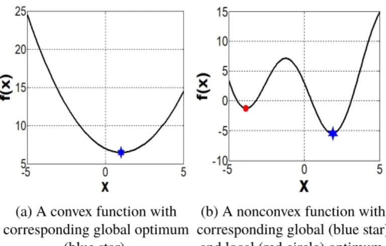
1.8. TERMINOLOGIES
Different terminologies used throughout the dissertation are defined here before delving into the problem formulation, beginning with global and local solutions. Figure 1.3a shows a function with its minimum (i.e., blue star). The blue star in Figure 1.3a is the global minimum of function since there is no point with a lower objective function value than this point. In Figure 1.3b, the red circle is the minimum point in a close neighboring region but it is not the global minimum for the function because there is another point (the blue star) with lower objective function than this point. Thus, the red circle is a local minimum and the blue star is the global minimum for the function.
(a) A convex function with corresponding global optimum
(blue star).
(b) A nonconvex function with corresponding global (blue star)
and local (red circle) optimum.
(c) A nonconvex function with corresponding global (blue star)
and local (red circle) optimum.
Figure 1.4. Illustrating of tight and loos relaxations for a nonconvex function.
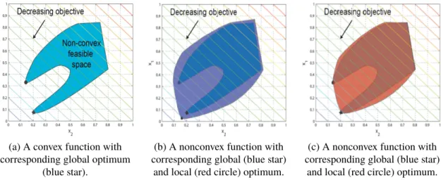
Another terminology that is used throughout the report is convex relaxation. A space is convex if and only if it contains all points on the line segments connecting every pair of points in that space. A convex relaxation encloses the feasible space of a non-convex problem in a larger non-convex space. Figure 1.4a illustrates a non-non-convex feasible space of an example optimization problem where black circle and star indicate the local and global optimum in the feasible space. A convex relaxation of feasible space is illustrated in Figure 1.4b where the global minimum of the original feasible space is not equal to the global minimum of convex relaxation of the problem. The relaxation gap is the difference between the global solution of original problem and the global solution of its convex relaxation. A non-zero relaxation gap implies that the convex relaxation for the problem can be further tightened. Conversely the convex relaxation provided for original function in Figure 1.4c is tight since the global optimum of the original problem and its convex relaxation are equal. The AC OPF problem is defined next.
PAPER
I. EMPIRICAL INVESTIGATION OF NON-CONVEXITIES IN OPTIMAL POWER FLOW PROBLEMS
ABSTRACT
Optimal power flow (OPF) is a central problem in the operation of electric power systems. An OPF problem optimizes a specified objective function subject to constraints imposed by both the non-linear power flow equations and engineering limits. These con-straints can yield non-convex feasible spaces that result in significant computational chal-lenges. Despite these non-convexities, local solution algorithms actually find the global optima of some practical OPF problems. This suggests that OPF problems have a range of difficulty: some problems appear to have convex or “nearly convex” feasible spaces in terms of the voltage magnitudes and power injections, while other problems can exhibit significant non-convexities. Understanding this range of problem difficulty is helpful for creating new test cases for algorithmic benchmarking purposes. Leveraging recently de-veloped computational tools for exploring OPF feasible spaces, this paper first describes an empirical study that aims to characterize non-convexities for small OPF problems. This paper then proposes and analyzes several medium-size test cases that challenge a variety of solution algorithms.
1. INTRODUCTION
The optimal power flow (OPF) problem seeks an optimal operating point for an electric power system in terms of a specified objective function (e.g., minimizing generation cost, matching a desired voltage profile, etc.). The feasible space for an OPF problem is dictated by equality constraints corresponding to the network physics (i.e., the power flow equations) and inequality constraints determined by engineering limits on, e.g., voltage magnitudes, line flows, and generator outputs. Non-linear constraints from the power flow equations and the engineering limits can result in non-convex feasible spaces. This paper applies an empirical approach to characterize typical non-convexities that occur in OPF feasible spaces. The geometric structures characterized in this paper are based on projections of the power injections and voltage magnitudes.
OPF problems may have multiple local optima [1] and are generally NP-Hard [2, 3], even for radial networks [4]. Since first being formulated by Carpentier in 1962 [5], a broad range of algorithms have been applied to solve OPF problems, including Newton-Raphson, sequential quadratic programming, interior point methods, etc. [6, 7]. Convergence of many algorithms only ensures local optimality, i.e., no feasible points in the solution’s immediate neighborhood have a better objective value. Other locally optimal points may exist outside of this immediate neighborhood, some of which may have substantially better objective values.
In contrast to local solvers, global algorithms seek the lowest-cost point in the entire feasible space. Provably obtaining the global solution is relevant for many analyses, such as multi-stage and robust optimization where providing any theoretical guarantees for the over-all problem requires certifying global optimality of solutions to certain subproblems [8, 9]. Moreover, the large scale of power systems means that even small percentage improvements in operational efficiency can have a significant aggregate impact [10], thus motivating the development of global algorithms.
Many recently developed global algorithms employ convex relaxation techniques, which enclose the feasible space of an OPF problem in a larger convex space. Optimizing over the convex space provides a lower bound for the OPF problem’s objective value, can certify OPF infeasibility, and, when the relaxation isexact, provides the globally optimal decision variables. A variety of convex relaxations are based on semidefinite programming (SDP) [2, 11–13] and second-order cone programming (SOCP) [14, 15]. Recent work is surveyed in [16].
For some practical OPF problems, these convex relaxations certify that the solutions obtained by local solvers are, in fact, globally optimal (or at least very near the global optimum) [2, 11–15, 17]. There also exist challenging test cases for which local solution algorithms may fail to yield globally optimal solutions and convex relaxations have large relaxation gaps [1, 18, 19]. Thus, the challenges inherent to solving OPF problems span a range of difficulties.
An OPF problem’s difficulty is closely related to convexity characteristics of the problem’s feasible space. The range of difficulties suggests that some OPF feasible spaces are “nearly convex” in terms of the voltage magnitudes and power injections, while others exhibit significant non-convexities. The development of sufficient conditions for exactness of some convex relaxation techniques [20] has implications for the convexity characteristics of a certain limited class of OPF problems [21]. In particular, these conditions imply that portions of the feasible spaces relevant to the minimization of active power generation are convex for OPF problems that satisfy non-trivial technical conditions. Previous work also shows that the feasible spaces of a more general class of OPF problems can have significant non-convexities [1, 22–30].
Although the existing literature makes significant progress, OPF convexity charac-teristics are not yet fully understood. This paper leverages two recently developed computa-tional tools to better understand non-convexities in OPF feasible spaces. The first tool is an algorithm for reliably computing discretized representations of OPF feasible spaces [28].
The second tool is a continuation algorithm that identifies multiple local optima for OPF problems [31].
Using these tools, this paper describes an empirical analysis to better understand causes of OPF non-convexities. This analysis randomly constructs many small OPF test cases. These test cases are not directly representative of realistic power systems due to their small sizes. However, large problems may have subregions with similar features. Moreover, experience with convex relaxations of large-scale problems suggests that non-convexities are often associated with small subregions of the system [11, 12]. Thus, exploring the characteristics of these small test cases can provide useful lessons for understanding non-convexities in large problems. After construction, the test cases are screened to identify those likely to have non-convexities using a process based on an SDP relaxation. The feasible space computation algorithm in [28] is applied to the screened cases to characterize their non-convexities.
Observations and test cases in [1] suggest the importance of binding lower limits on voltage magnitudes and reactive power generation with regard to OPF non-convexities. All non-convexities characterized in our numerical experiment are also related to the lower limits on voltage magnitudes and reactive power generation. Our numerical experiment thus suggests that non-convexities are more frequently associated with lower limits on voltage magnitudes and reactive power generation than other constraints, at least for problems in the parameter ranges considered in our experiment.
This paper then extends the insights gained from this numerical experiment to develop challenging medium-size OPF problems based on modifications to the IEEE test cases. Modifying the system loading, voltage limits, and reactive power limits yields OPF problems where lower limits on voltage magnitudes and reactive power generation are binding. The resulting OPF problems have multiple local optima and challenge state-of-the-art convex relaxation techniques.
In addition to empirically validating the insights gained from small problems, these medium-size test cases can serve to exercise both local and global OPF solution algorithms. While convex relaxations are exact or close to exact for many previous test cases [19], the medium-size test cases developed in this paper have large optimality gaps between the best-known local solutions and the bounds from the convex relaxations. In order to determine whether the optimality gaps are due to poor local optima or poor bounds, we apply both a random search technique and the continuation algorithm in [31] in order to find additional local optima. This approach yields several additional local solutions and many stationary points, but none with a better objective value than that obtained via the local solver in Matpower [32]. This may suggest that the optimality gaps are due to a poor bound from the relaxations, thus motivating the development of improved convex relaxation techniques. This paper is organized as follows. Section 2 overviews the OPF problem. Sec-tion 2.1 reviews computaSec-tional tools for studying OPF feasible spaces. SecSec-tion 3 describes the numerical experiment that is the first main contribution of this paper. Using insights from the small test cases, Section 4 presents and studies challenging OPF problems derived by modifying several IEEE test cases, which is the second main contribution of this paper. Section 5 concludes the paper.
2. OVERVIEW OF THE OPF PROBLEM
This section overviews the OPF problem and its SDP relaxation. Further details are provided in [2, 10, 11].
Consider ann-bus system, whereN “ t1, . . . ,nuis the set of buses,Gis the set of generator buses, andL is the set of lines. LetY denote the network admittance matrix. Let
PDk ` jQDk represent the active and reactive load demand at bus k P N, where j is the imaginary unit. LetVk represent the voltage phasor at busk PN, with the angle ofV1equal to zero to set the angle reference. Define the rank-one matrixW “VVH P Hn, whereHn
upper and lower limits. Buses without generators have maximum and minimum generation set to zero. Define a convex quadratic cost of active power generation with coefficients
c2,k ě0, c1,k, andc0,k for k P G.
Each linepl,mq PL is modeled by an ideal transformer with turns ratioτlmejθlm: 1 in series with aΠ circuit with mutual admittance ylm and total shunt susceptance j bsh,lm. Define ek as the kt h column of the identity matrix. Let p¨q, p¨q|, and p¨qH denote the complex conjugate, transpose, and complex conjugate transpose, respectively. Define the matrices Hk “ YHe ke | k`eke | kY 2 , H˜k “ YHe ke | k´eke | kY 2j , Flm “ 1 τ2 lm pylm´j bsh,lm{2qele|l ´ ylm{`τlme´jθlm˘emel|, andFml “ pylm´ j bsh,lm{2qeme|m´ylm{ ` τlmejθlm˘ele|m. The OPF problem is
min VPCn ÿ kPG c2,kptrpHkWq `PDkq2 `c1,kptrpHkWq `PDkq `c0,k (1a) subject to PkminďtrpHkWq `PDk ďPkmax @k PN (1b) Qmink ďtrpH˜kWq `QDk ďQmaxk @k PN (1c) ` Vkmin˘2ďtr`eke|kW˘ď`Vkmax˘2 @k PN (1d) tr “` Flm`FlmH ˘ W‰(2` tr “ j`FlmH ´Flm ˘ W‰(2 ď4 ` Slmmax˘2 @ pl,mq PL (1e) tr “` Fml`FmlH ˘ W‰(2` tr “ j`FmlH ´Fml ˘ W‰(2 ď4 ` Slmmax˘2 @ pl,mqL (1f) W “VVH (1g)
where trp¨qis the trace. Constraints (1b)–(1d) are linear in the entries ofW. The objec-tive (1a) and line flow constraints (1e)–(1f) are convex in the entries ofW. Thus, all the non-convexity in (1) is contained in the rank constraint (1g).
The numerical experiment in Section 3 uses an SDP relaxation of the OPF problem as part of a screening step to identify test cases which may have relevant non-convexities. This SDP relaxation is formed by replacing (1g) with a positive semidefinite constraint
W ľ 0 [2]. The solution to the SDP relaxation provides a lower bound on the OPF problem’s optimal objective value. If the condition rankpWq “ 1 is satisfied, the lower bound provided by the SDP relaxation is exact. Conversely, if rankpWq ą 1, the lower bound may be strictly below the OPF problem’s global optimum. Anoptimality gapis then computed as the percent difference between the objective values for a local solution to (1) and the lower bound from the SDP relaxation. A non-negligible optimality gap suggests the possible presence of a non-convexity in the OPF problem’s feasible space near the global solution.
Note that the OPF problem formulation (1) does not consider some possible sources of non-convexity that are present in more general OPF problem formulations (e.g., con-tingency constraints, discrete devices such as switched shunts, models of uncertainty, etc.) [8, 33–35]. A variety of approaches address these possible sources of non-convexity (e.g., branch-and-bound and cutting plane methods for discrete variables [36], chance-constrained formulations [33–35], etc.). Many of these approaches solve the OPF formula-tion (1) as a subproblem within a broader algorithm. Therefore, identifying non-convexities inherent to the OPF formulation (1) is relevant to a wide range of problems. Future work will study the impacts of other types of OPF constraints on the feasible spaces’ convexity characteristics.
2.1. TOOLS FOR STUDYING OPF FEASIBLE SPACES
This section first describes an algorithm that computes the feasible space (i.e., the set of points satisfying (1b)–(1g)) for small OPF problems and then discusses approaches for finding multiple local optima. The numerical experiments in the following sections employ both of these algorithms to characterize OPF non-convexities.
![Figure 1.1. Explanation of the variables in the DistFlow equations for line pi, kq P L [7].](https://thumb-us.123doks.com/thumbv2/123dok_us/1455444.2694744/26.918.286.692.118.226/figure-explanation-variables-distflow-equations-line-pi-kq.webp)